Precision and High-Resolution Mapping of Quantitative Trait Loci by Use of Recurrent Selection, Backcross or Intercross Schemes

(1)



Precision and High-Resolution Mapping of Quantitative Trait Loci by Use of

Recurrent Selection, Backcross or Intercross Schemes

Z. W. Luo,*

,†,1

_{Chung-I Wu}

‡

**_{and M. J. Kearsey*}**

*School of Biosciences, The University of Birmingham, Edgbaston, Birmingham B15 2TT, England,†_{Laboratory of Population} and Quantitative Genetics, Institute of Genetics, Fudan University, Shanghai 200433, China and

‡_{Department of Ecology and Evolution, The University of Chicago, Chicago, Illinois 60637}

Manuscript received October 10, 2001 Accepted for publication March 13, 2002

ABSTRACT

Dissecting quantitative genetic variation into genes at the molecular level has been recognized as the greatest challenge facing geneticists in the twenty-first century. Tremendous efforts in the last two decades were invested to map a wide spectrum of quantitative genetic variation in nearly all important organisms onto their genome regions that may contain genes underlying the variation, but the candidate regions predicted so far are too coarse for accurate gene targeting. In this article, the recurrent selection and backcross (RSB) schemes were investigated theoretically and by simulation for their potential in mapping quantitative trait loci (QTL). In the RSB schemes, selection plays the role of maintaining the recipient genome in the vicinity of the QTL, which, at the same time, are rapidly narrowed down over multiple generations of backcrossing. With a high-density linkage map of DNA polymorphisms, the RSB approach has the potential of dissecting the complex genetic architecture of quantitative traits and enabling the underlying QTL to be mapped with the precision and resolution needed for their map-based cloning to be attempted. The factors affecting efficiency of the mapping method were investigated, suggesting guidelines under which experimental designs of the RSB schemes can be optimized. Comparison was made between the RSB schemes and the two popular QTL mapping methods, interval mapping and composite interval mapping, and showed that the scenario of genomic distribution of QTL that was unlocked by the RSB-based mapping method is qualitatively distinguished from those unlocked by the interval mapping-based methods.

T

HE benchmark article by Lander and Botstein very low (ⵑ5%). Little progress has been made so far (1989) stimulated enormous interest in locating in cloning quantitative trait genes on the basis of in-quantitative trait loci (QTL) in experimental and natu- ferred map location of QTL despite the claim inAlpert ral populations. Research efforts in the last decade were andTanksley(1996) that a yeast artificial chromosome focused on mass production of high-throughput DNA (YAC) clone bearing a major QTL affecting fruit weight polymorphic markers (Dibet al.1996;Wanget al.1998; in tomato was successfully obtained. However, the gene

Marthet al.2001) and development of analytical meth- (fw2.2) was finally identified after 20 years’ journey in

ods for detecting the presence and inferring the loca- narrowing down the candidate genomic region that con-tions of QTL in marker linkage maps (Lander and tains fw2.2(Fraryet al.2000).

Botstein 1989; Haley and Knott 1992; Luo and Theoretical investigations (Boehnke1994;Guo and

Kearsey1992;Zeng1994;Rabinowitz1997;Mottet Lange 2000) suggested that the major bottleneck in

al.2000). A recent comprehensive review based on 47 narrowing down the confidence interval of QTL loca-experimental studies of QTL mapping in plants, how- _{tion is the limited number of informative meioses} ob-ever, revealed that the current QTL mapping practice _{tainable in most mapping populations in the literature.} entails tremendous research effort and financial invest- _{Experimental strategies using historically accumulated} ment but yields QTL map localizations that are far from _{recombinations between markers and QTL have been} being satisfactory for identifying and isolating the quan- _{suggested as an efficient approach to improving map} titative trait genes at the molecular level (Kearseyand _{resolution of QTL. These include several alternatives.}

Farquhar1998). The analysis showed that QTL were _First, _Darvasi _and _Soller _{(1995) demonstrated that}

usually mapped with low accuracy and poor resolution _{the confidence interval of QTL location inferred from} (ⵑ10–30 cM) and that the proportion of quantitative _{a conventional F}

2 mapping population might be re-genetic variation determined by the QTL detected was _{duced by up to fivefold if the F}

2population is expanded into a so-called advanced intercross line (AIL) by contin-ued intercross. Improvement in the mapping resolution

1_{Corresponding author:}_{School of Biosciences, The University of}

Bir-in an AIL is due to breakdown of lBir-inkage disequilibrium

mingham, Edgbaston, Birmingham B15 2TT, England.

E-mail: [email protected] between the QTL and their linked marker loci.

(2)

ever, an appropriate statistical method still needs to be breeding scheme. An alternative way, suggested inHill (1998), is to intersperse one generation of intercrossing developed to model and analyze the data from an AIL

experiment (ManlyandOlson1999). Second, the rate among the selected individuals between consecutive backcrossings. However, it is less clear what impact the of dissipation in linkage disequilibrium between QTL

and nearby marker loci in genetically isolated natural recurrent selection backcrossinter seintercross (RSBI) scheme will have on maintaining QTL of small effect populations with good genealogical records may be

modeled in terms of the recombination fraction be- on the one hand and on separating the QTL from their surrounding marker loci on the other. Moreover, many tween the loci and demographic parameters defining

the evolutionary history of the populations. This ap- important questions remain to be answered. How can the basic idea of RSB or RSBI be extended to dissect proach may, in the best case, enable QTL to be located

in a region of ⬍1 cM (Hill and Weir 1994; de la complex genetic variation into QTL? How robust is the strategy to various models of QTL effect? What precision

ChapelleandWright1998;Luoet al.2000;Luoand

Wu2001). However, it must be pointed out that much and resolution in the QTL mapping may be expected by use of the RSB or RSBI schemes if advantage is fully uncertainty exists in this population-based analysis if

evolutionary details of the populations are not appropri- taken of the fast development of single nucleotide polymorphic (SNP) markers? The extremely dense dis-ately taken into account (Zollnerandvon Haeseler

2000). Statistical modeling of linkage disequilibrium tribution of SNP markers over the whole genome may provide at least one polymorphic site in each of the involved with QTL has arisen as a new challenge to

modern quantitative genetics (Luoet al.2000;Luoand functional genes in the genome (Marthet al. 2001), thus allowing full control of the genetic architecture Wu2001). Third, use of congenic lines was shown to

be effective in narrowing intervals of inferred QTL loca- that underlies complex quantitative genetic variation. What are the major factors affecting the RSB or RSBI tion, providing the QTL effect was so significant that

genotypes at the QTL could be assigned accurately for their efficiency in QTL mapping? In an attempt to address these questions, this article provides an exact (Darvasi1997;NadeauandFrankel2000). Another

major limitation of this approach is that tightly linked theoretical prediction of mean and variance of heterozy-gosity at a marker locus linked to one or two QTL with QTL would not be resolved if their genetic effects act

in the same direction in the congenic strains. Fourth, any degree of recombination for any number of genera-tions of the RSB schemes. This builds up a theoretical construction of chromosome substitution lines enables

precise identification of the chromosomes, which carry basis for the RSB-based QTL mapping. More compli-cated models were investigated and the above questions QTL. Recombinant progeny from backcrossing the

ap-propriate chromosome substitution strain to its host were explored by numerical evaluation of the theoreti-cal predictions and by extensive computer simulation. strain may be used to test whether more than one QTL

accounts for trait phenotypic difference among the sub- Comparisons were made between the RSB(I) strategy and the routine methods of QTL mapping for their stitution chromosomes and to locate each QTL with

considerable map resolution (Nadeauet al.2000). precision and resolution in identifying locations of mul-tiple linked QTL.

A breeding scheme with repeated backcrossing and selection was proposed long ago byWright(1952) for isolating quantitative trait genes of large effect, but little

THEORY AND METHODS progress was made in QTL analysis until a recent series

of elegant theoretical studies byHill(1997, 1998). On The breeding scheme:The theoretical analysis consid-ers a breeding scheme initiated from two inbred lines the basis of his theory of directional selection for

quanti-tative traits in finite populations (Hill1969), he formu- P1 and P2 that are assumed to be fixed for different alleles atmmarker loci andqloci affecting a quantitative lated the probability that quantitative trait genes of

spec-ified effects remain segregating in a backcross family trait. The QTL alleles increasing the phenotype are fixed in P1and those decreasing the phenotype in P2. undergoing one generation of truncation selection for

nonrecurrent parental phenotype. The results were ex- Effects of individual QTL are scaled in units of standard deviation of the residual variation of the trait, which tended to multiple generations by an approximation

that did not take into account the change in gene fre- are assumed to be normally distributed with mean zero and variance 1.0. Various models for genetic effects of quency under repeated selection and random drift. Use

of multiple generations in the recurrent selection back- the QTL are considered in the following analysis. The two inbred lines are crossed to generate an F1 cross (RSB) scheme is essential for accumulating a

suf-ficient amount of recombination both between closely family and a random sample of F1individuals are back-crossed to recurrent parental line P2to produceF inde-linked QTL and between the QTL and nearby markers.

It has been clear that the RSB is an effective approach pendent backcross families with a constant size of N. These families are defined as the first generation of the only in isolating QTL of large effect from their

(3)

Figure1.—A diagram illustrat-ing a recurrent selection and back-cross (RSB) breeding scheme.

titative trait are selected. The selected individuals are at any marker loci, which may or may not be linked to the QTL in any generation of the breeding program. either backcrossed to the recurrent parent or randomly

intercrossed to produce the next generation of the fami- In all QTL mapping strategies, map location of a pu-tative QTL is inferred from information of marker ge-lies. The breeding program lasts forTgenerations. Let

Bit(SBit) orIit(SIit) denote theith backcross or intercross notype and trait phenotype observed from a specified

mapping population. In the RSB scheme, the genetic family (i ⫽ 1, 2, . . . , F) at generation t before (or

after) selection. A simple diagram describing the RSB contribution of QTL to the trait phenotype is reflected as efficiency of selection in counterbalancing against breeding scheme is given in Figure 1.

Hill (1997, 1998) exploited the probability that the loss of the QTL allele of the nonrecurrent parent due to repeated backcross and genetic drift, while the genes at one or two QTL of specified effects remain

segregating after one generation of truncation selec- genetic marker in the system provides information about genome location and extent to which the selec-tion. This provides a direct comparison with the

situa-tion where the probability is reduced by one-half, on tion affects it. The closer the marker locus is to the selected locus (QTL), the more efficient the selection average, if the locus is free of the selection pressure.

(4)

heterozygous status. Therefore, the marker heterozy- In general, gosity serves as a natural and rational measure for its

location relative to the QTL. When the genome regions ptR⫽Pr兵Xt⫽R其⫽

兺

S

Pr兵Yt⫺1⫽S其Pr兵Xt⫽R|Yt⫺1⫽S其⫽

兺

S qt⫺1S␩tRS bearing QTL are covered with densely distributed

mark-ers, the closest approximation for map location of the qtS⫽Pr兵Yt⫽S其⫽

兺

R

Pr兵Xt⫽R其Pr兵Yt⫽S|Xt⫽R其⫽

兺

R

ptR␰tSR. (2) QTL may be inferred as the location at which the marker

heterozygosity reaches its peak value. Thus, the

theoreti-cal analyses below are focused on heterozygosity of a _{In the above,}_兺_R_(or_兺_S_{) represents summation over all} marker locus that is linked to QTL with an arbitrary _possible_r_k_{under the constraint}_兺4

k⫽1rk⫽N(orskunder

value of recombination frequency. _兺4

k⫽1sk⫽n). The conditional probability can be

calcu-The theoretical analyses comprise four sections. calcu-The _{lated as} first two relate to the dynamic change in genetic

struc-ture of the RSB breeding populations under two loci

␰tSR⫽Pr

兵

Yt⫽S|Xt⫽R

其

⫽

兿

4

k⫽1

冢

rk

sk

冣

兺

4

i⫽1

siIi(S,R;␮) (3)

(one marker and one QTL) and three loci (one marker and two QTL) models. The third section develops the

in which calculation of the mean and variance of the marker

heterozygosity under the above two models. When the

RSB scheme is interrupted by incorporation of inter- Ii(S,R;␮)⫽

冮

∞

⫺∞

[1⫺ ⌽i(x)]si⫺1

兿

4

j⫽1

⌽j(x)rj⫺sj

兿

4

j⬆i

[1⫺ ⌽j(x)]sjfi(x)dx,

crossing, prediction of the dynamic change in linkage

(4) disequilibria between multiple loci becomes intractable.

To investigate the impact of the RSBI, theoretical

analy-where ␮ ⫽(␮1 ␮2 ␮1␮2)⬘and␮1 and␮2are means of sis is restrained to one QTL only and described in the

QTL genotypes Aa andaa, respectively, and fi(x) and

last section.

⌽i(x) are, respectively, the probability density function

Two loci model: The model considers one marker

and the probability distribution function of a normal locus and one QTL. The two alleles at the marker locus

distribution with mean␮iand variance 1.0,

are denoted byMandm, respectively, and those at the QTL byAanda.For each of theFindependent

back-cross families, letXt⫽ (xt1xt2xt3xt4)TandYt⫽(yt1yt2yt3 ␩tRS ⫽Pr

兵

Xt⫽ R|Yt⫺1 ⫽S

其

⫽ N!

兿

4

k⫽1rk!

兿

4

k⫽1

φrk_k_, ₍₅₎

yt4)⬘ be the two vectors that represent the distribution of four possible genotypes, at generationt, inBit(before

whereφ1⫽(1 ⫺c)s1/2N,φ2⫽[(1⫺c)s1⫹2s2⫹s3⫹ selection) and inSBit(after selection), respectively. In

s4]/2N,φ3 ⫽[cs1⫹ s3]/2N, andφ4⫽[cs1⫹ s4]/2N. other words, elementxti(oryti) is a random variable for

Three loci model:There are three possible patterns

the number of individuals with genotypejinBit(orSBit),

of relative locations of one marker locus and two QTL wherej⫽1, 2, 3, 4 corresponding, respectively, to joint

under this model. Letc1and c2 be recombination fre-genotypes MA/ma, ma/ma, mA/ma, and Ma/ma at the

quencies between loci 1 and 2 and between loci 2 and marker and QTL.

3, respectively. Assuming there is no recombination in-The stochastic change in population genetic structure

terference, the recombination frequency between the during a RSB program is described fully by the following

first and the third loci will be c⫽c1(1⫺ c2)⫹c2(1 ⫺ probability distributions:

c1). Analogous to the above two loci model, the breeding ptR⫽Pr

兵

Xt⫽ R

其

⫽Pr

兵

xtk⫽rk,k⫽1, 2, 3, 4

其

scheme at generationtcan be described by two random

兵

Xt⫽R

其

⫽Pr

兵

xtk⫽rk,k⫽1, 2, . . . , 8

其

These can be evaluated in a recursive formulation that

is initiated from ⫽

_兺

S

Pr

兵

Yt⫺1⫽S

其

Pr

兵

Xt⫽R|Yt⫺1⫽S

其

⫽

兺

S

qt⫺1S␩tRS (6)

p1R⫽Pr兵X1⫽R其⫽

N!

2N

兿

4

k⫽1rk!

(1⫺c)r1⫹r2_cr3⫹r4

qtS⫽Pr

兵

Yt⫽S

其

其

⫽

兺

R

ptR␰tSR. (7)

(5)

These can be evaluated from the initial condition and if the marker locates at the right of the linked QTL,

p1R⫽

N! 2N

兿

8

k⫽1rk!

[(1⫺c1)(1⫺c2)]r1⫹r2

⫻[c1(1⫺c2)]r3⫹r4_[(1⫺_c1₎_c2_]r5⫹r6₍_c1c2₎r7⫹r8 (8)

G⫽          

(1⫺c1)(1⫺c2)/2 0 0 0

(1⫺c1)(1⫺c2)/2 1 1/2 (1⫺c2)/2

c1(1⫺c2)/2 0 1/2 0

c1(1⫺c2)/2 0 0 (1⫺c2)/2

c1c2/2 0 0 0

c1c2/2 0 0 c2/2

(1⫺c1)c2/2 0 0 0

(1⫺c1)c2/2 0 0 c2/2

and the conditional probabilities

␰tSR⫽Pr兵Yt⫽S|Xt⫽R其

⫽

_兿

8 k⫽1

冢

rk sk

冣

兺

8

i⫽1

si

冮

∞

⫺∞

[1⫺ ⌽i(x)]si⫺1

兿

8

j⫽1

⌽j(x)rj⫺sj

兿

8

j⬆i

[1⫺ ⌽j(x)]sjfi(x)dx (9)

␩tRS⫽Pr兵Xt⫽R|Yt⫺1⫽S其⫽

N!

兿

8

k⫽1rk!

兿

8

k⫽1

␭rk_k, (10)

0 0 0 0

[(1⫺c1)(1⫺c2)⫹c1c2]/2 1/2 (1⫺c1)/2 1/2

[c1(1⫺c2)⫹(1⫺c1)c2]/2 0 c1/2 0

0 0 0 0

[(1⫺c1)(1⫺c2)⫹c1c2]/2 0 0 0

0 1/2 c1/2 0

0 0 (1⫺c1)/2 0

[c1(1⫺c2)⫹(1⫺c1)c2]/2 0 0 1/2

          .

wherefi(x) and⌽i(x) are defined similarly to those in

Equation 4.⌳ ⫽(␭1␭2. . .␭8)⬘can be calculated from product of matricesGandS⫽ (s1s2. . . s8)⬘as

Mean and variance of the marker heterozygosity:The

⌳ ⫽ 1

NGS⬘, (11) marginal probabilities␲tk⫽Pr{xtk⫽rk} and␲tij⫽Pr{xti⫽ ri,xtj⫽rj} can be computed from the above joint

proba-bility distributions as␲tk⫽Rl⬆kPr{xtl⫽ rl,l⫽1, 2, . . . ,

where the matrix G has a form that depends on the

K|兺K

i⫽1ri ⫽ N} and ␲tij ⫽兺l⬆i∧j Pr{xtl ⫽ rl,l⫽ 1, 2, . . . ,

relative location of the marker to the QTL. If the marker

K|兺K

i⫽1ri⫽ N} withK⫽4 or 8 for the two or three loci

locates at the left side of the linked QTL,

model, respectively. Thus, the expected mean and vari-ance of the marker heterozygosity can be calculated as

Ht⫽

冦

1

N

兺

N

i⫽1(␲t1⫹ ␲t3)i for the two loci model 1

N

兺

N

i⫽1(␲t1⫹ ␲t4⫹ ␲t5⫹ ␲t8)i for the three loci model

G⫽          

(1⫺c1)(1⫺c2)/2 0 0 0

(1⫺c1)(1⫺c2)/2 1 1/2 [(1⫺c1)(1⫺c2)⫹c1c2]/2

c1c2/2 0 1/2 [c1(1⫺c2)⫹c2(1⫺c1)]/2

c1c2/2 0 0 [(1⫺c1)(1⫺c2)⫹c1c2]/2

(1⫺c1)c2/2 0 0 0

(1⫺c1)c2/2 0 0 [c1(1⫺c2)⫹c2(1⫺c1)]/2

c1(1⫺c2)/2 0 0 0

(12)

and

Vt⫽

F⫺1

N2_F

冦

兺

N

i⫽1

(␲t1⫹ ␲t3)i2⫹2

兺

N

i⫽0

兺

N

j⫽0

␲t13ij⫺

冤

兺

N

i⫽0

(␲t1⫹ ␲t3)i

冥

2

冧

0 0 0 0

(1⫺c1)/2 1/2 (1⫺c2)/2 1/2

c1/2 0 c2/2 0

0 0 0 0

(1⫺c1)/2 0 0 0

0 1/2 c2/2 0

0 0 (1⫺c2)/2 0

c1/2 0 0 1/2

          ; ₍₁₃₎

for the two loci model or

when the marker is between the linked QTL, _V_t_⫽F⫺1

N2_F

冦

兺

N

i⫽1

(␲t1⫹ ␲t4⫹ ␲t5⫹ ␲t8)i2

⫹2

兺

N

i⫽0

兺

N

j⫽0

(␲t14⫹ ␲t15⫹ ␲t18⫹ ␲t45⫹ ␲t48⫹ ␲t58)ij

G⫽          

(1⫺c1)(1⫺c2)/2 0 0 0

(1⫺c1)(1⫺c2)/2 1 1/2 (1⫺c2)/2

c1(1⫺c2)/2 0 1/2 0

c1(1⫺c2)/2 0 0 (1⫺c2)/2

(1⫺c1)c2/2 0 0 0

(1⫺c1)c2/2 0 0 c2/2

c1c2/2 0 0 0

c1c2/2 0 0 c2/2

⫺

冤

_兺

N i⫽0

(␲t1⫹ ␲t4⫹ ␲t5⫹ ␲t8)i

冥

2

冧

(14)

for the three loci model. In theory, the above analysis may be extended to any number of marker loci and QTL but the algebra involved would be very tedious.

Recurrent selection and backcross or intercross

scheme:Here we exploited the impact of introducing

intercross among the selected individuals into the RSB

0 0 0 0

(1⫺c1)/2 1/2 [(1⫺c1)(1⫺c2)⫹c1c2]/2 1/2

c1/2 0 [c1(1⫺c2)⫹(1⫺c1)c2]/2 0

0 0 0 0

(1⫺c1)/2 0 0 0

0 1/2 [c1(1⫺c2)⫹(1⫺c1)c2]/2 0

0 0 [(1⫺c1)(1⫺c2)⫹c1c2]/2 0

c1/2 0 0 1/2

          ;

(6)

xti (or yti) are a random number of individuals with whose complete sequence data are available (i.e., yeast,

Caenorhabditis elegans, Drosophila, Arabidopsis, etc.) or genotypei in one of the independent families before

(or after) selection (i ⫽ 1, 2, 3 corresponding to the are to be available (i.e., human, mice, pig, cattle, rice, etc.). Second, use of extremely dense marker maps QTL genotypesAA,Aa, andaarespectively). Probability

distributions of these random vectors are given by allows us to exploit the maximum efficiency of the RSB mapping strategy in identifying the QTL map locations. ptR⫽Pr

兵

Xt⫽R

其

⫽Pr

兵

xtk⫽rk,k⫽1, 2, 3

其

_{Numerical analyses:} _{For a given set of parameters}

defined in the previous theoretical analysis, the mean

⫽

_兺

兵

ytk⫽sk,k⫽1, 2, 3

其

difficulty in the numerical analysis is the limitation in

computer time and memory for evaluating Equations 2, 6, and 7. These equations involve summation of a

⫽

_兺

_兿

3

j⬆i

[1⫺ ⌽j(x)]sjfi(x)dx. (16) _{configurations of}_r

i (i⫽ 1, 2, . . . ,K withK ⫽4 or 8

under the two and three loci model, respectively) such The conditional probability ␩(X)

tRS depends on whether _that _N ⫽ 兺K

i⫽1ri. A general formula for this number is

the selected individuals are backcrossed to the recurrent _{given by}_c₍_K_,_N₎_⫽

_兿

K

i⫽2(N ⫹i⫺1)/(K⫺1)!, which line (X⫽B) or intercrossed to each other (X⫽I) and _{takes a value of 264,385,836 when}_K_⫽ _{8 and}_N_⫽ _50.

has forms as _{Thus, numerical analysis demonstrated here has to be}

restricted to the cases with a small family size. ␩(B)

tRS ⫽

冢

n

r2

冣

[(2s1 ⫹s2)/n]r2[(s2⫹2s3)/n]r3 (17) Figure 2 illustrates distributions of the means and variances of heterozygosity at 100 marker loci that were linked with (a) one, (b) two, or (c) three QTL in the ␩(I)

tRS ⫽

N!

兿

3

k⫽1rk!

兿

3

k⫽1 φrk

k, (18)

various RSB breeding programs. Figure 2, a and b, was obtained from theoretical predictions and Figure 2c was where φ1 ⫽ [4s1(s1 ⫺1) ⫹ 2s1s2 ⫹ s2(s2 ⫺ 1)]/4n(n ⫺ _{calculated from averages of 100 repeated simulations} 1), φ2 ⫽[2s1s2⫹ 4s1s3 ⫹s2(s2 ⫺1) ⫹2s2s3]/2n(n⫺ 1) _{of the RSB scheme whose parameters were given as the} andφ3⫽ [s2(s2⫺ 1)⫹2s2s3⫹4s3(s3⫺ 1)]/4n(n⫺1). _{scheme 1 in Table 1. The pattern of change in the mean} The dynamics of the probability distributions can be _{and variance of heterozygosity maintained at the marker} readily evaluated using the initial condition p1R ⫽ _{loci directly reflected their locations relative to that of}

Pr{X1 ⫹R}⫽ (n!/r2!r3!)(1/2)(r₂⫹r₃)_{. Similarly, the mean}

the QTL. The peak of the mean curves always occurred and variance of heterozygosity at the QTL in generation _{at the same locations as the QTL regardless of the QTL} tof the RSBI scheme are given byHt⫽兺Ni⫽1␲t2i/Nand _{effects and the other parameters. On the other hand,}

Vt⫽

[

兺Ni⫽1␲t2i2⫺

(

兺Ni⫽1␲t2i

)

2

]

⫻(F⫺1)/N2F, respec- _{there was a rapid decline in the marker heterozygosity as}

tively. _{its mapping distance from the QTL increased. However,}

the change in the variance over the marker loci showed two different patterns. Whenever there was a substantial NUMERICAL ANALYSES AND SIMULATION STUDY

(7)

Figure

2.—Expected

value

(solid

symbols)

and

the

variance

(open

symbols)

of

heterozygosity

at

the

m

arker

loci

linked

to

varying

numbers

of

QTL

under

d

iffere

nt

design

parameters:

(a)

one

QTL

and

all

schemes

with

T

⫽

20;

(b)

two

QTL

and

all

schemes

with

n

⫽

2,

N

⫽

10,

F

⫽

50,

and

T

⫽

20;

(c)

three

QTL

and

all

schemes

with

n

⫽

5,

N

⫽

50,

F

⫽

20,

a

nd

h

2⫽

0.5;

a

nd

(d)

one

QTL

and

all

schemes

with

n

⫽

5,

N

⫽

50,

F

⫽

20,

and

d

⫽

0.5,

where

n

,

N

,

F

,

T

,

h

2,a

n

d

are

accordingly

the

number

o

f

individuals

selected,

the

family

size,

the

number

of

families,

the

number

o

f

g

enerations

of

consecutive

selection

a

nd

backcrossing,

heritability,

and

a

dditive

effect

of

QTL.

Red

arrows

indicate

location

o

f

the

(8)

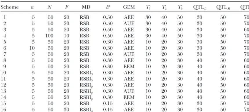
TABLE 1

The parameters defining the 16 simulated breeding schemes

Scheme n N F MD h2 _GEM _T1 _T2 _T3 _QTL

L QTLM QTLR

1 5 50 20 RSB 0.50 AEE 30 40 50 30 50 70

2 5 50 20 RSB 0.50 AUE 30 40 50 30 50 70

3 5 50 20 RSB 0.50 AEE 30 40 50 30 50 60

4 5 100 10 RSB 0.50 AEE 30 40 50 30 50 70

5 5 50 20 RSB 0.30 AEE 10 20 30 30 50 70

6 10 50 20 RSB 0.30 AEE 10 20 30 30 50 70

7 5 50 20 RSB 0.30 AUE 10 20 30 30 50 70

8 5 50 20 RSB 0.30 AEE 10 20 30 40 50 60

9 5 50 20 RSB 0.30 EEM 10 20 30 40 50 60

10 5 50 20 RSBI3 0.30 AEE 10 20 30 40 50 60

11 5 50 20 RSBI5 0.30 AEE 10 20 30 40 50 60

12 5 50 20 RSBIp 0.30 AEE 10 20 30 40 50 60

13 5 50 20 RSBIp 0.30 AUE 10 20 30 40 50 60

14 5 50 20 RSBIp 0.30 EEM 10 20 30 40 50 60

15 5 50 20 RSB 0.15 AEE 10 20 30 30 50 70

16 5 50 30 RSBIp 0.15 AEE 10 20 30 30 50 70

n,N, andFare the number of selected individuals, the size of each family, and the number of families. The three mating designs (MD) are RSB, recurrent selection and backcross; RSBIk, recurrent selection, backcross

at everykgeneration otherwise intercross; and RSBIp, recurrent selection, backcross whenever family phenotypic

mean reaches that of backcross family at the first generation otherwise intercross.h2_{, heritability of the trait.} The three QTL genetic effect models (GEM) are AEE, additive and equal effect; AUE, additive unequal effect; and EEM, epistatic effect model.Ti (i⫽1, 2, 3) is the generation time at which the marker heterozygosity

was surveyed; QTLX(X⫽ L, M, R) are the locations of the left, middle, and right QTL on the simulated

chromosome.

ing effect of the selected locus on the nearby neutral at the QTL with small effect in the RSB breeding pro-gram. However, the program may be improved in prop-markers depends on the selection efficiency at the

se-lected locus and the linkage disequilibrium between the erly designed experiments. For a given number of indi-viduals involved in the experiment, the breeding selected and the neutral loci. The low heterozygosity

maintained at the selected locus indicates low effective- scheme with larger family sizes but smaller number of families (scheme 2 in Figure 2a) was superior in main-ness of selection at the locus and thus the dynamics

of heterozygosity at the nearby marker loci were less taining a high level of heterozygosity to that with smaller family size but larger number of families (scheme 3 in affected by hitchhiking but dominated by genetic drift.

This resulted in a much lower allele frequency at the Figure 2a). Selection intensity played a significant role in slowing down the allele loss at QTL due to genetic marker loci and thus a smaller variance in their allele

frequencies. In contrast, a high gene frequency at the drift, particularly when the QTL had a low genetic con-tribution to the trait. Figure 2b presents the analysis of QTL reflects that the influence of genetic drift on

fre-quency is effectively counterbalanced by selection. The two linked QTL under three models of genetic effects: (i) the additive and equal effect model (schemes 1 and strong hitchhiking effect maintained a high gene

fre-quency for those markers in the vicinity of the selected 4), where the two QTL contributed equally and addi-tively to the trait; (ii) the additive and unequal effect loci before complete breakage of linkage disequilibria

between the QTL and markers, while drift in the marker model (scheme 2) under which the two QTL affected the trait additively but the first QTL had twice as large gene frequencies was balanced less effectively than that

in the QTL gene frequencies. Thus, a larger variance an effect as the second QTL; and (iii) the epistatic model (scheme 3), where the individuals carrying the in gene frequency might be observed at these markers

than at the nearby selected loci. The analysis revealed trait-increasing allele at each of the two QTL had a genotypic value that was fourfold those carrying only that not only the mean but also the variance of the

marker heterozygosity provide essential information re- one such allele. A distinct feature observed from com-paring the three models is that epistasis had remarkable garding locations of the QTL and regarding how genes

at both QTL and marker loci in the RSB populations influence on the marker heterozygosity. Under the epi-static model, the individuals carrying the increasing al-evolve under a complicated combination of

evolution-ary factors of recombination, genetic drift, and selec- lele at every QTL had a much better chance of being selected in comparison to the corresponding additive tion.

(9)

nonre-combinant gametes carrying all increasing alleles to be selection and either intercrossing or backcrossing when-ever the family mean at generationtwas not lower than selected and in turn results in a substantial increase in

the level of heterozygosity at these loci on the one hand that at generation 1 (RSBIp). Intercrossing was

simu-lated as random mating among the selected individuals. and a noticeable decrease in recombination between

the loci on the other. This includes the possibility of selfing of some selected

individuals, but this would not seriously influence our Loss of heterozygosity at the QTL with small effect

was very fast in the RSB program. Reducing the amount results. The parameters defining the 16 simulated schemes are listed in Table 1. Each of the simulated schemes of backcrossing by incorporation of intercrossing into

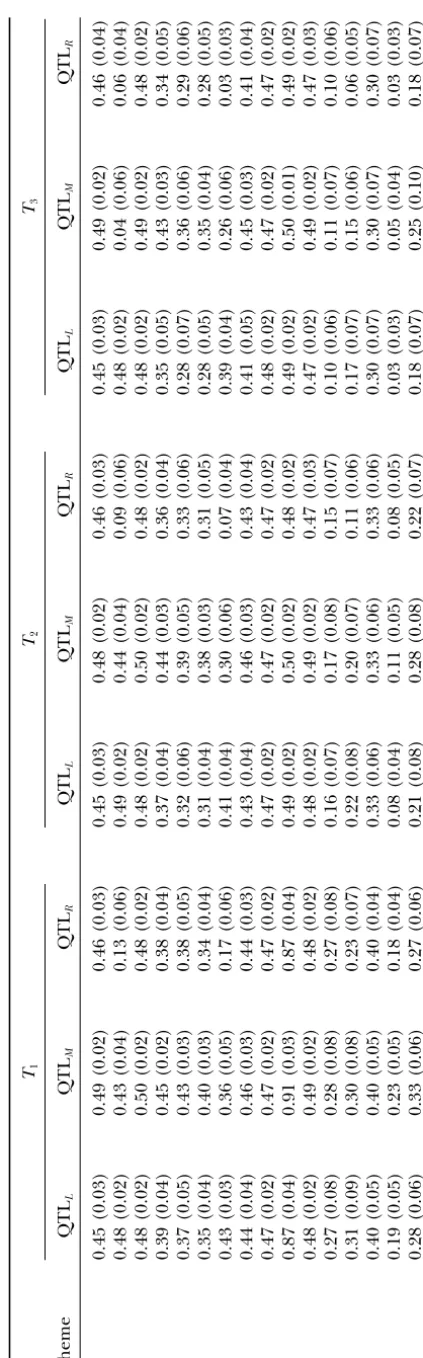
the program was effective in slowing down the allelic loss was repeated 100 times unless otherwise stated. Means and standard deviations of heterozygosity main-particularly when intercrossing was frequent (scheme 2

in Figure 2d), but this caused a large fluctuation in the tained at the QTL were calculated from the repeated simulation trials for all these simulated schemes and are gene frequency. The effect of the RSBI on inferring the

QTL locations is discussed in the following simulation illustrated in Table 2. It can be seen from the table that there was a general trend in loss of heterozygosity at study.

Simulation study:We developed a series of computer the QTL as the breeding schemes evolved (fromT1to

T3). However, the rate of loss of the heterozygosity was simulation programs that offer a high degree of

flexibil-ity in mimicking the RSB or RSBI schemes specified influenced by almost all parameters defining the breed-ing program. Heritability was a dominant factor influ-with various mating design parameters, different genetic

architectures of quantitative traits, and arbitrary linkage encing the RSB schemes. Given the other parameters, the selected alleles at the QTL, which contributed 50% relationships between the marker loci and QTL. In a

single meiosis, the “random walk” procedure has been of phenotypic variance, were maintained at an un-changed frequency after 50 generations of RSB (scheme described elsewhere (LuoandKearsey1992) to

simu-late genetic recombination between linked loci. Chias- 1), whereas the alleles had almost completely vanished after 30 generations of RSB if the QTL explained only mata interference, sexual differentiation in

recombina-tion frequency, and segregarecombina-tion distorrecombina-tion were assumed 15% of the phenotypic variance (scheme 15). However, incorporation of intercrossing in the RSB breeding to be absent in the simulation model.

As described in the above numerical analysis, we con- schemes was effective in reducing loss of the increasing alleles at the QTL (scheme 16). Comparison of heterozy-sidered only one chromosome in the simulation study.

There were 100 evenly distributed marker loci on the gosity at the QTL between schemes 15 and 16 revealed that use of family phenotypic mean was an effective chromosome, 3 of them affecting a quantitative trait.

Map distance between adjacent loci is constantly 1 cM. way to determine the switch between backcrossing and intercrossing during the breeding program such that For a given proportion of quantitative genetic variation

explained by the 3 QTL (h2_{), three models under which} _{the selected alleles may be effectively protected from} being lost. As has been shown in the previous numerical h2_{was resolved into genetic effect of QTL were}

consid-ered to investigate robustness of the mapping strategy analysis, the genetic model of the QTL effect influenced the heterozygosity loss remarkably. Epistasis in the QTL to various QTL effect models. These include (i) the

additive equal effect (AEE) model, under which each effects dramatically slowed down the loss of the QTL heterozygosity (scheme 9) compared to the correspond-allele increasing the trait delivered an additive

contribu-tion ofd ⫽ [2h2_/3(1⫺ _h2_)]1/2 _{to the trait phenotype;} _{ing additive models (schemes 7 and 8). A higher level} of heterozygosity was maintained at more closely linked (ii) the additive unequal effect (AUE) model, under

which genetic effects of the increasing alleles at the QTL (scheme 9) than at the less closely linked QTL (scheme 5). For a given experimental size (N⫻F), the three QTL are, respectively,d,d/2, andd/4 withd ⫽

[32h2_/21(1_⫺_h2_)]1/2_{; and (iii) the epistatic effect model} _{scheme with larger family size but smaller number of} families (scheme 4) was more effective than the scheme (EEM), under which any individual carryingk(ⱕ2)

in-creasing alleles would have a genotypic effect of [2kh2_/3 _{with smaller family size but larger number of families} (scheme 1) for maintenance of the heterozygosity at (1 ⫺ h2_)]1/2_{, but the genotypic effect was 2.0 when it}

carried all 3 increasing alleles (i.e.,k⫽3). The individ- the selected loci.

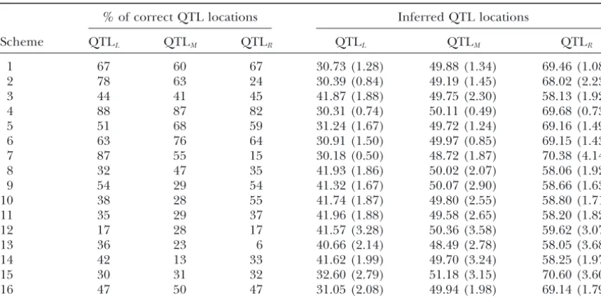
Locations of the QTL were inferred in the simulation ual phenotype was determined by its genotypic effect

plus a number that was randomly sampled from a stan- study as locations of the marker loci at which the hetero-zygosity curve at generation 30 reached the peak values, dard normal distribution.

The breeding program was initiated withFbackcross and the accuracy in locating the QTL was evaluated as the percentage of the peak values of the same curve families obtained from two homozygous inbred parental

lines, which were fixed with different alleles at the 100 occurring at the simulated QTL locations in repeated simulations. Tabulated in Table 3 were the percentages loci. After the start of the breeding program, three

mat-ing strategies might be performed: (i) RSB, (ii) recur- of the correct locations of the QTL and means and standard deviations of the inferred QTL locations. It rent selection and either intercrossing or backcrossing

(10)

of QTL mapping was size of the QTL genetic effect. The QTL with effect as large as 1.23 units of the residual standard deviation was located correctly in 87% of the repeated simulation trials, but the accuracy dropped to only 15% if the effect was quartered (scheme 17). As the trait had a very low heritability, increasing alleles at the QTL were almost completely lost after 30 genera-tions of RSB (refer to scheme 15 in Table 2) and the QTL in this scheme was poorly mapped. However, the loss in mapping accuracy was substantially recovered in scheme 16 in which the RSBIpwas performed. The actual

map distance between linked QTL showed an obvious influence on their mapping accuracy: The closer the QTL were linked, the poorer their mapping accuracy (scheme 1 vs. 3). For a given experimental size, the QTL in the scheme with a larger family size but smaller number of families (scheme 4) were located more accu-rately than those with a smaller family size but larger number of families (scheme 1). Comparison between schemes 5 and 6 showed that the QTL in the scheme under a stronger selection had resulted in a worse rather than a better mapping precision of QTL. Epistasis in the QTL genetic effects was preferred in the RSB schemes for a better maintenance of genetic heterozy-gosity at the loci (Table 2), but it hindered rather than improved accumulation of recombination between the QTL and between them and the nearby marker loci and thus resulted in a reduced accuracy.

Although there was variation in the percentage of correct identification of the QTL locations over the various schemes considered in the simulation, the QTL in all these schemes were, on average, mapped to loca-tions that were not significantly different from their actual map locations. The standard deviations of the estimated QTL locations were in the range of 0.49–4.14 cM, and the change in the standard deviation among the different breeding schemes was consistent with change in the percentage of correct QTL locations in-ferred.

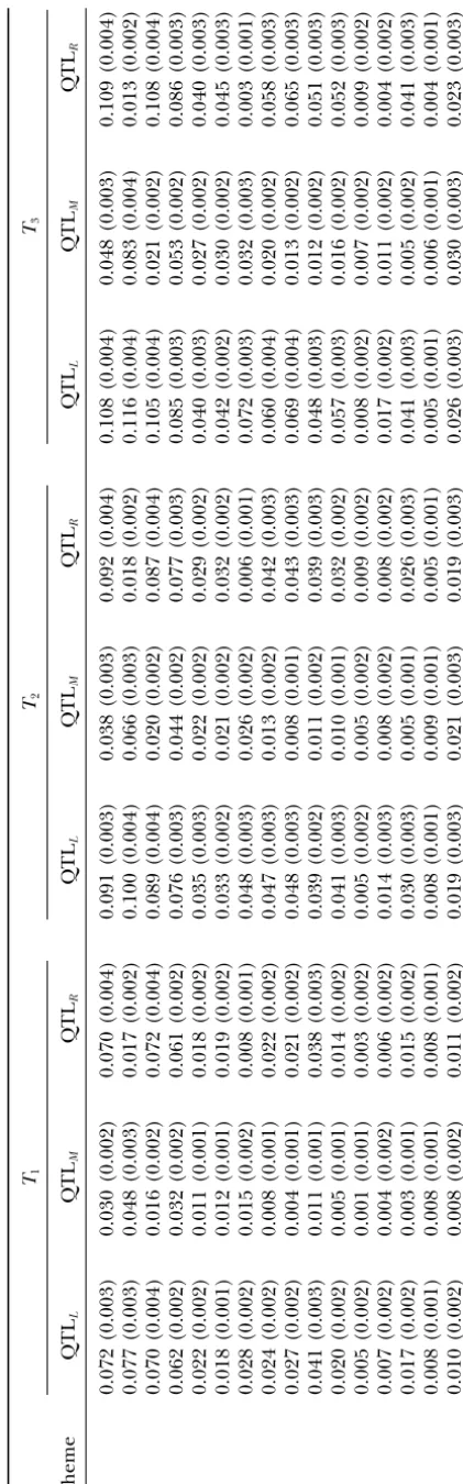
The above discussion represented evaluation of preci-sion in mapping QTL under the RSB or RSBI schemes. It is important to exploit resolution of QTL mapping by use of the marker heterozygosity distribution. Anad hocmeasure of resolution for an estimated QTL location at theith marker locus can be␭i⫽Hi⫺(Hi⫺1⫹Hi⫹1)/ 2, whereHidenotes the heterozygosity of theith marker

locus. Means and standard errors of the resolution esti-mates over repeated simulations of all the schemes are tabulated in Table 4. It can be seen that all parameters considered here influenced the mapping resolution. As expected, there was a trend of improvement in the mapping resolution as the breeding schemes pro-gressed, provided a substantial amount of heterozygosity was maintained at the stage when the QTL locations were examined. When the other parameters were fixed, the trait heritability played an important role in

de-TABLE 2 Means a nd standard deviations (in parentheses) of heterozygosity maintained at the QTL at different generation times in the simulated breeding sche mes T1 T2 T3 Scheme QTL L QTL M QTL R QTL L QTL M QTL R QTL L QTL M QTL R 1 0 .45 (0.03) 0.49 (0.02) 0.46 (0.03) 0 .45 (0.03) 0.48 (0.02) 0.46 (0.03) 0.45 (0.03) 0.49 (0.02) 0.46 (0.04) 2 0 .48 (0.02) 0.43 (0.04) 0.13 (0.06) 0 .49 (0.02) 0.44 (0.04) 0.09 (0.06) 0.48 (0.02) 0.04 (0.06) 0.06 (0.04) 3 0 .48 (0.02) 0.50 (0.02) 0.48 (0.02) 0 .48 (0.02) 0.50 (0.02) 0.48 (0.02) 0.48 (0.02) 0.49 (0.02) 0.48 (0.02) 4 0 .39 (0.04) 0.45 (0.02) 0.38 (0.04) 0 .37 (0.04) 0.44 (0.03) 0.36 (0.04) 0.35 (0.05) 0.43 (0.03) 0.34 (0.05) 5 0 .37 (0.05) 0.43 (0.03) 0.38 (0.05) 0 .32 (0.06) 0.39 (0.05) 0.33 (0.06) 0.28 (0.07) 0.36 (0.06) 0.29 (0.06) 6 0 .35 (0.04) 0.40 (0.03) 0.34 (0.04) 0 .31 (0.04) 0.38 (0.03) 0.31 (0.05) 0.28 (0.05) 0.35 (0.04) 0.28 (0.05) 7 0 .43 (0.03) 0.36 (0.05) 0.17 (0.06) 0 .41 (0.04) 0.30 (0.06) 0.07 (0.04) 0.39 (0.04) 0.26 (0.06) 0.03 (0.03) 8 0 .44 (0.04) 0.46 (0.03) 0.44 (0.03) 0 .43 (0.04) 0.46 (0.03) 0.43 (0.04) 0.41 (0.05) 0.45 (0.03) 0.41 (0.04) 9 0 .47 (0.02) 0.47 (0.02) 0.47 (0.02) 0 .47 (0.02) 0.47 (0.02) 0.47 (0.02) 0.48 (0.02) 0.47 (0.02) 0.47 (0.02) 10 0.87 (0.04) 0.91 (0.03) 0.87 (0.04) 0 .49 (0.02) 0.50 (0.02) 0.48 (0.02) 0.49 (0.02) 0.50 (0.01) 0.49 (0.02) 11 0.48 (0.02) 0.49 (0.02) 0.48 (0.02) 0 .48 (0.02) 0.49 (0.02) 0.47 (0.03) 0.47 (0.02) 0.49 (0.02) 0.47 (0.03) 12 0.27 (0.08) 0.28 (0.08) 0.27 (0.08) 0 .16 (0.07) 0.17 (0.08) 0.15 (0.07) 0.10 (0.06) 0.11 (0.07) 0.10 (0.06) 13 0.31 (0.09) 0.30 (0.08) 0.23 (0.07) 0 .22 (0.08) 0.20 (0.07) 0.11 (0.06) 0.17 (0.07) 0.15 (0.06) 0.06 (0.05) 14 0.40 (0.05) 0.40 (0.05) 0.40 (0.04) 0 .33 (0.06) 0.33 (0.06) 0.33 (0.06) 0.30 (0.07) 0.30 (0.07) 0.30 (0.07) 15 0.19 (0.05) 0.23 (0.05) 0.18 (0.04) 0 .08 (0.04) 0.11 (0.05) 0.08 (0.05) 0.03 (0.03) 0.05 (0.04) 0.03 (0.03) 16 0.28 (0.06) 0.33 (0.06) 0.27 (0.06) 0 .21 (0.08) 0.28 (0.08) 0.22 (0.07) 0.18 (0.07) 0.25 (0.10) 0.18 (0.07)

(11)

heri-TABLE 3

The percentage of correctly inferred QTL locations and means and standard deviations (in parentheses) of estimated QTL map locations

% of correct QTL locations Inferred QTL locations

Scheme QTLL QTLM QTLR QTLL QTLM QTLR

1 67 60 67 30.73 (1.28) 49.88 (1.34) 69.46 (1.08)

2 78 63 24 30.39 (0.84) 49.19 (1.45) 68.02 (2.23)

3 44 41 45 41.87 (1.88) 49.75 (2.30) 58.13 (1.92)

4 88 87 82 30.31 (0.74) 50.11 (0.49) 69.68 (0.73)

5 51 68 59 31.24 (1.67) 49.72 (1.24) 69.16 (1.49)

6 63 76 64 30.91 (1.50) 49.97 (0.85) 69.15 (1.43)

7 87 55 15 30.18 (0.50) 48.72 (1.87) 70.38 (4.14)

8 32 47 35 41.93 (1.86) 50.02 (2.07) 58.06 (1.92)

9 54 29 54 41.32 (1.67) 50.07 (2.90) 58.66 (1.63)

10 38 28 55 41.74 (1.87) 49.80 (2.55) 58.80 (1.71)

11 35 29 37 41.96 (1.88) 49.58 (2.65) 58.20 (1.82)

12 17 28 17 41.57 (3.28) 50.36 (3.58) 59.62 (3.07)

13 36 23 6 40.66 (2.14) 48.49 (2.78) 58.05 (3.68)

14 42 13 33 41.62 (1.99) 49.70 (3.24) 58.25 (1.97)

15 30 31 32 32.60 (2.79) 51.18 (3.15) 70.60 (3.60)

16 47 50 47 31.05 (2.08) 49.94 (1.98) 69.14 (1.79)

tability, the better the QTL was resolved. In contrast (CIM;Zeng1994) methods under the constraint of a constant capacity of genotyping 1000 individuals for 100 to its positive effect on maintenance of heterozygosity,

linked and evenly spaced marker loci. Of the marker epistasis in the QTL genetic effect showed a negative

loci, 3 were assumed to be QTL, which explained 30% of influence on the mapping resolution of the QTL due to

phenotypic variance of a quantitative trait. Map distance a reduced number of recombinants between the linked

between any pair of adjacent marker loci was 1 cM (ⵑ1% QTL and between them and their nearby marker loci

recombination frequency). For the IM and CIM analy-during the selection and backcrossing process. This

ef-ses, a backcross family with 1000 individuals was gener-fect was more obvious with the QTL surrounded by

ated and analyzed by use of the QTL cartographer other QTL. Population designs with smaller family size

(Bastenet al.1994), the computer software for carrying but larger number of families (i.e., scheme 1) were more

out the IM and CIM analyses. The RSB breeding effective in achieving a better mapping resolution.

Bet-schemes were simulated with 20 independent families ter resolution observed in such designs may be

ex-and 50 individuals for each of these families, yielding the plained by the fact that with larger numbers of families

same population size as the interval mapping analyses. there is a better chance of maintaining a wider range

Selection in the RSB program was for 50 generations of different recombinants between the linked QTL

at a constant intensity of 10%. It has already been themselves and between the QTL and the marker.

Selec-pointed out in the above simulation study that both tion intensity was less important for mapping resolution.

mean and variance of the marker heterozygosity are Comparison of the mapping resolution between the

informative about relative locations of the marker loci RSB schemes and the RSBI schemes showed that

reduc-to the selected QTL. To combine the information from ing the number of backcrossing generations and

these two statistics, a measure for the QTL presence was allowing intercrossing in a RSB scheme had reduced

the mapping resolution. More frequent intercrossing calculated as ␶it ⫽ Hit/

√

Vit when Vit ⬎ 0 otherwise 0,

whereHitandVitare, respectively, the mean and variance

tended to worsen the mapping resolution providing

frequent backcrossing had not driven the increasing of theith marker heterozygosity at generationt. Illustrated in Figure 3 are the distribution of the likeli-allele at the QTL to a very low frequency.

Comparison of the RSB schemes to the interval map- hood-ratio test statistics from the IM and CIM analyses

and the distribution of the measure of the QTL presence

ping-based methods:Interval mapping and its later

ex-tended versions have been the most popular methods in in the RSB schemes. It was very clear from analysis of the RSB schemes that the QTL locations were accurately QTL mapping in man, plants, and animals. This section

compares the RSB-based QTL mapping approach with and unambiguously identified as the chromosome loca-tions at which␶it reached its peak value. In addition,

the two most popularly cited interval mapping methods

in the literature: the interval mapping (IM;Landerand the method was very robust to various models of the QTL effects on the trait. The presence of the QTL on the

(12)

simulated chromosome was strongly evident from the interval mapping methods, but in sharp contrast, it did not provide clear-cut inference of the locations of the QTL. The interval mapping predictions of the QTL loca-tions worsened when there was epistasis in the QTL effects.

DISCUSSION

The present article develops a theoretical framework for predicting the mean and variance of heterozygosity maintained at marker loci linked to one or two QTL for any number of generations using the recurrent selection and backcross schemes previously proposed byWright (1952) and studied by Hill (1998). The theoretical prediction takes appropriate account of the dynamic change in linkage disequilibria between the QTL them-selves and between the QTL and the marker loci due to selection, recombination, and genetic drift during the breeding program. In principle, it is tractable to extend the analysis to more than the three loci modeled here because the distribution of multiple loci linkage disequilibria under the present setting is equivalent to that under a multiple loci haplotype model of linkage disequilibria. Nevertheless, numerical evaluation of the multiple loci system will be computationally very de-manding when the experimental size is large. More com-plicated models were investigated in the simulation study. The analyses demonstrated that distributions of mean and variance of heterozygosity at different marker loci in the RSB breeding program provide sufficient information regarding their relative locations to the QTL under selection in the program and regarding the evolutionary driving factors behind the breeding populations. Appropriate use of these statistics may pro-vide a simple but efficient alternative approach for map-ping complex quantitative genetic variation at a substan-tially improved precision and resolution. The major features of the RSB-based QTL mapping schemes can be summarized as follows:

1. The mapping strategy is powerful in identifying the polymorphic sites, which are in close linkage (i.e., 1 or 2 cM) to the QTL. Use of the dense marker maps that include the genomic polymorphisms within the QTL (cSNP, for instance) enables precise identifica-tion of the map locaidentifica-tions of the QTL. In general, the error in the inference of the QTL locations will not be beyond one or two times the coverage density of the marker maps.

2. Maintenance of the selected genes at a nontrivial frequency is a prerequisite for achieving both preci-sion and resolution in inferring their map locations under the RSB framework. For QTL with large ge-netic effects on the trait phenotype, selection on the trait is usually efficient enough to counterbalance dilution of the recipient genome regions around the

TABLE 4 Means a nd standard errors (in parentheses) of the resolution for the QTL mapping at different generation times in the simulated breeding schemes T1 T2 T3 Scheme QTL L QTL M QTL R QTL L QTL M QTL R QTL L QTL M QTL R 1 0.072 (0.003) 0.030 (0.002) 0.070 (0.004) 0.091 (0.003) 0.038 (0.003) 0.092 (0.004) 0.108 (0.004) 0.048 (0.003) 0 .109 (0.004) 2 0.077 (0.003) 0.048 (0.003) 0.017 (0.002) 0.100 (0.004) 0.066 (0.003) 0.018 (0.002) 0.116 (0.004) 0.083 (0.004) 0 .013 (0.002) 3 0.070 (0.004) 0.016 (0.002) 0.072 (0.004) 0.089 (0.004) 0.020 (0.002) 0.087 (0.004) 0.105 (0.004) 0.021 (0.002) 0 .108 (0.004) 4 0.062 (0.002) 0.032 (0.002) 0.061 (0.002) 0.076 (0.003) 0.044 (0.002) 0.077 (0.003) 0.085 (0.003) 0.053 (0.002) 0 .086 (0.003) 5 0.022 (0.002) 0.011 (0.001) 0.018 (0.002) 0.035 (0.003) 0.022 (0.002) 0.029 (0.002) 0.040 (0.003) 0.027 (0.002) 0 .040 (0.003) 6 0.018 (0.001) 0.012 (0.001) 0.019 (0.002) 0.033 (0.002) 0.021 (0.002) 0.032 (0.002) 0.042 (0.002) 0.030 (0.002) 0 .045 (0.003) 7 0.028 (0.002) 0.015 (0.002) 0.008 (0.001) 0.048 (0.003) 0.026 (0.002) 0.006 (0.001) 0.072 (0.003) 0.032 (0.003) 0 .003 (0.001) 8 0.024 (0.002) 0.008 (0.001) 0.022 (0.002) 0.047 (0.003) 0.013 (0.002) 0.042 (0.003) 0.060 (0.004) 0.020 (0.002) 0 .058 (0.003) 9 0.027 (0.002) 0.004 (0.001) 0.021 (0.002) 0.048 (0.003) 0.008 (0.001) 0.043 (0.003) 0.069 (0.004) 0.013 (0.002) 0 .065 (0.003) 10 0.041 (0.003) 0.011 (0.001) 0.038 (0.003) 0.039 (0.002) 0.011 (0.002) 0.039 (0.003) 0.048 (0.003) 0.012 (0.002) 0 .051 (0.003) 11 0.020 (0.002) 0.005 (0.001) 0.014 (0.002) 0.041 (0.003) 0.010 (0.001) 0.032 (0.002) 0.057 (0.003) 0.016 (0.002) 0 .052 (0.003) 12 0.005 (0.002) 0.001 (0.001) 0.003 (0.002) 0.005 (0.002) 0.005 (0.002) 0.009 (0.002) 0.008 (0.002) 0.007 (0.002) 0 .009 (0.002) 13 0.007 (0.002) 0.004 (0.002) 0.006 (0.002) 0.014 (0.003) 0.008 (0.002) 0.008 (0.002) 0.017 (0.002) 0.011 (0.002) 0 .004 (0.002) 14 0.017 (0.002) 0.003 (0.001) 0.015 (0.002) 0.030 (0.003) 0.005 (0.001) 0.026 (0.003) 0.041 (0.003) 0.005 (0.002) 0 .041 (0.003) 15 0.008 (0.001) 0.008 (0.001) 0.008 (0.001) 0.008 (0.001) 0.009 (0.001) 0.005 (0.001) 0.005 (0.001) 0.006 (0.001) 0 .004 (0.001) 16 0.010 (0.002) 0.008 (0.002) 0.011 (0.002) 0.019 (0.003) 0.021 (0.003) 0.019 (0.003) 0.026 (0.003) 0.030 (0.003) 0 .023 (0.003)

(13)

Figure

3.—Comparison

o

f

the

RSB

schemes

to

interval

mapping

(IM)

a

nd

composite

interval

mapping

(CIM)

of

a

trait

controlled

by

three

QTL,

which

explained

30%

of

phenotypic

variation

under

d

ifferent

models

of

their

genetic

effects

and

varying

m

apping

distances

between

linked

QTL:

(a)

additive

equal

QTL

eff

ect

and

2

0

cM

b

etween

adjacent

QTL,

(b)

a

dditive

unequal

QTL

effect

and

2

0

cM

b

etween

adjacent

QTL,

(c)

epistatic

QTL

effect

and

2

0

cM

between

a

djacent

QTL,

and

(d)

epistatic

QTL

effect

and

1

0

cM

b

etween

adjacent

QTL.

The

red

arrow

indicates

the

simulated

location

o

f

the

(14)

drift that causes loss of the selected genes over the a mapping resolution as close as 1 cM or less. In contrast, there is an upper limit in marker density by breeding process. Selection in the RSB schemes is

usually not able to prevent QTL with small effects which the efficiency of the interval mapping methods will not be improved further (LanderandSchork from quick gene fixation. Instead of repeatedly

back-crossing the selected individuals to the recurrent pa- 1994). On the other hand, the informative meioses are practically limited in the segregating populations rental line, incorporation of intercrossing among the

selected individuals at some stages of the breeding for which the interval mapping methods were devel-oped. These make the QTL mapping inferred from program is effective in maintaining the selected QTL

alleles for long enough to break down linkage dis- the methods far from satisfactory at the same crite-rion as the RSB mapping results (Figure 3). The RSB equilibrium between the QTL and the nearby marker

loci so that the QTL may be isolated from their closely mapping approach is robust to errors in estimation

linked genome regions. of map distances between the marker loci whereas

3. Many factors that can be managed by experimental- methods based on interval mapping are sensitive to ists play an important role in determining success of these errors (LuoandKearsey1992). The practical the RSB-based approach in the QTL mapping. The implementation of the RSB mapping schemes does number of generations of the breeding program af- not need any complicated statistical modeling of the fects the degree of breakage in linkage disequilibria experimental data. Given that many years of consid-between the QTL and consid-between them and their erable research efforts to isolate genes affecting com-nearby marker loci. A prerequisite for precision and plex traits have resulted in slow progress, we would high-resolution mapping of the QTL using this pro- not consider the long duration of the RSB breeding gram is sufficient breakage of the linkage disequilib- program to be an expensive investment for signifi-ria. In principle, the theory developed in this study cant improvement in mapping precision and resolu-can easily be extended to provide the estimate of the tion in the QTL locations that may lead directly to number of generations required to reach indepen- cloning of QTL. It may not be strictly appropriate to dent segregation between the linked QTL and be- compare the multiple generation approach of RSB-tween the QTL and their linked marker loci. After based QTL mapping to interval mapping analysis, establishment of linkage equilibrium between these which is based on the populations of a single segre-loci, selection will maintain a slow change in gene _{gating generation. Among the several multiple} gen-frequency at the QTL and, at the same time, genetic _{eration approaches suggested in the literature, use} drift will drive the marker gene to be fixed very _{of the advanced intercross line has been shown} theo-quickly, yielding a clear scenario of the QTL locations _{retically to have potential for improving mapping} as showed in Figure 3. For a given size of experiment _{resolution of QTL localization (Darvasi}_and_Soller and whenever possible, experimental designs with _1995;_Xiong_and_Guo_{1997). These researchers} con-a lcon-arger fcon-amily but smcon-aller number of fcon-amilies con-are _{sistently revealed a diminished return in the} resolu-superior in reducing the effect of genetic drift and _{tion improvement after eight generations of} contin-thus maintaining higher allele frequencies at the se- _{ued intercross in an AIL scheme. This property of} lected loci, but may be inferior in obtaining a better _{the AIL approach is in sharp contrast to that of the} mapping resolution of the QTL in comparison to _{RSB scheme in which the mapping resolution has} the designs with smaller family size but a larger num- _{been observed in our study to increase steadily as the}

ber of families. _{breeding scheme progresses until complete breakage}

4. The RSB-based QTL mapping approach is quite ro- _{of linkage disequilibrium between the QTL and their} bust to various models of genetic effects of QTL _{linked marker loci. However, a direct and} compre-even though there is a difference in the mapping _{hensive comparison between these two schemes} re-resolution for the QTL affecting quantitative traits _{quires that an appropriate statistical method be} es-under different models of genetic effects. Positive _{tablished to analyze experimental data from these} epistasis in the QTL effects enhanced effectiveness _{breeding schemes.}

of their selection. This resulted in two consequences:

Selection in the RSB breeding program is based entirely an increased heterozygosity at the QTL but a

de-on the trait phenotype. Appropriate use of marker infor-creased resolution in their mapping when compared

mation will be an effective way of improving the effi-to the corresponding additive model.

ciency of selection for the QTL with small effects (Luo 5. The QTL mapping approach discussed above has

et al.1997). The marker-assisted RSB mapping will en-several advantages over the interval mapping method

able not only the QTL of large effects but those with and its extended versions. It takes full advantage of

small effects to be maintained during the breeding pro-a dense mpro-arker mpro-ap pro-and uses pro-accumulpro-ated

recombi-cedure, and thus the complete genetic architecture un-nations between the QTL and their nearby marker

derlying the polygenic variation will, in principle, be loci. This yields precise identification of the QTL