ABSTRACT
GOWDA, BHARATH DODDE. Numerical Study of Homogeneous Charge Compression Ignition Combustion in a H2-fueled Engine. (Under the direction of Dr. Tarek Echekki.)
Homogeneous charge compression ignition (HCCI) engines fueled by hydrogen have the po-tential to provide cost-effective power with high efficiencies and very low emissions. They can also play a vital role in the transition to a hydrogen-based energy economy. Challenges related to combustion control and operational limits have to be tackled in order for this technol-ogy to be able to compete with existing diesel- and gasoline-based powertrains. The present study is carried out to investigate the abilities of various injection strategies to prepare an ideal in-cylinder mixture and control the autoignition process. Computations are performed using a stand-alone one-dimensional turbulence (ODT) model formulated for engine simulations.
This work is carried out in two parts. In the first part, two of the most commonly used injection methods, port fuel injection (PFI) and single-pulse direct injection (DI), are used to prepare the air-fuel mixture. The mixture distribution, conditions at ignition and the modes of combustion are studied and compared. It is found that direct injection is able to prepare a more uniformly lean mixture and control the autoignition more effectively than port fuel injection. A combi-nation of ignition modes are found to be operating when PFI is used as compared to mainly volumetric autoignition in the case of DI. Also, DI is able to maintain lower temperatures and achieve reduced NOxemissions.
c
Copyright 2011 by Bharath Dodde Gowda
Numerical Study of Homogeneous Charge Compression Ignition Combustion in a H2-fueled Engine
by
Bharath Dodde Gowda
A thesis submitted to the Graduate Faculty of North Carolina State University
in partial fulfillment of the requirements for the Degree of
Master of Science
Mechanical Engineering
Raleigh, North Carolina
2011
APPROVED BY:
Dr. William Roberts Dr. Tiegang Fang
DEDICATION
To
Mom, Susheela Gowda, Dad, Dodde Gowda, Brother, Punith Doddegowda,
BIOGRAPHY
Bharath Dodde Gowda was born on 5 March 1986 in Bangalore, the Silicon Valley and Garden City of India. He completed his secondary schooling at St. Germain High School and Bishop Cotton Boys’ School and graduated with the Indian School Certificate in March 2004. He attended the National Institute of Technology, Karnataka (NITK), located in Surathkal, India, for his undergraduate studies and earned a Bachelor of Technology (B.Tech) in Mechanical Engineering degree in May 2010.
Bharath developed a passion for research while working as a Summer Research Assistant under Dr. K. P. Jagannath Reddy at the High Enthalpy Aerodynamics Lab, Indian Institute of Science, Bangalore. He also had the opportunity to work for Mercedes-Benz Research & Development India Pvt. Ltd. as a Student Intern in the Fuel Cell Simulation and Modeling group. These experiences led him to develop a keen interest in the area of Thermal and Fluid Sciences.
ACKNOWLEDGEMENTS
I would like to express my gratitude to my advisor, Dr. Tarek Echekki, whose help and guid-ance played a crucial role in the successful completion of this thesis. I am also grateful to Dr. William Roberts and Dr. Tiegang Fang for serving as members of my advisory committee and providing valuable insight and suggestions.
I thank my labmates, Andreas, Fu, Hessam, Jaehyung, Joey, Kamlesh, Patrick, Sami, Shubham, Sumit, and Yajuvendra for their support as well as some great social times. I also thank my friends and roommates in Raleigh, Gult, Karthik, Bakshi, Sriram, Lopa and Prachi for all their love and support over the past two years.
TABLE OF CONTENTS
List of Tables . . . vii
List of Figures . . . viii
Chapter 1 Introduction . . . . 1
1.1 Homogeneous Charge Compression Ignition (HCCI) Combustion . . . 3
1.1.1 Advantages of HCCI Mode Operation . . . 5
1.1.2 Issues and Challenges . . . 6
1.2 Hydrogen as a Fuel . . . 8
1.3 Review of Literature on HCCI Combustion . . . 9
1.4 One Dimensional Turbulence (ODT) . . . 14
1.5 Objective . . . 15
1.6 Overview . . . 16
Chapter 2 Numerical Setup . . . . 17
2.1 Domain Specification . . . 19
2.2 Assumptions . . . 20
2.3 Momentum Conservation . . . 22
2.4 Species Mass Conservation . . . 25
2.5 Energy Conservation . . . 28
2.6 Constitutive Relations . . . 32
2.6.1 Ideal Gas Law . . . 32
2.6.2 Piston Speed . . . 33
2.7 Summary of the ODT Model Equations . . . 34
2.8 Numerical Implementation . . . 36
Chapter 3 Port Fuel Injection & Direct Injection Simulations . . . . 41
3.1 Motivation . . . 41
3.2 Run Conditions . . . 42
3.2.1 Port Fuel Injection . . . 45
3.2.2 Direct Injection . . . 45
3.3 Results and Discussion . . . 46
3.3.1 Ignition Maps . . . 47
3.3.2 Mixture Formation . . . 50
3.3.3 Autoignition & Combustion Characteristics . . . 54
3.3.4 Parametric Study of DI HCCI Combustion . . . 71
3.3.5 NOxFormation . . . 85
Chapter 4 Multiple Injection Strategies . . . 89
4.1 Motivation . . . 89
4.2 Run Conditions . . . 91
4.3 Results and Discussion . . . 94
4.3.1 Mixture Formation . . . 96
4.3.2 Autoignition and Combustion Modes . . . 105
4.4 Conclusions . . . 127
Chapter 5 Summary and Future Work . . . 129
5.1 Summary . . . 129
5.2 Future Work . . . 132
LIST OF TABLES
Table 2.1 H2/Air reaction mechanism. . . 38
Table 2.2 Common parameters used in simulations . . . 39
Table 3.1 Common mixture and flow conditions for PFI & DI simulations . . . 43
Table 3.2 PFI-specific run conditions . . . 45
Table 3.3 DI-specific run conditions . . . 46
Table 3.4 Common mixture and flow conditions for parametric study of DI-HCCI . 72 Table 3.5 Computation points for parametric study of DI-HCCI . . . 73
Table 3.6 Ignition delay times for DI-HCCI with varying fueling rates . . . 75
Table 3.7 Ignition delay times for DI-HCCI with varying injection velocities . . . . 77
Table 3.8 Ignition delay times for DI-HCCI with varying compression ratios . . . . 79
Table 3.9 Ignition delay times for DI-HCCI with varying engine RPM . . . 81
Table 3.10 Ignition delay times for DI-HCCI with varying induction pressures . . . 83
Table 3.11 Ignition delay times for DI-HCCI with varying EGR volume . . . 85
Table 4.1 Common mixture and flow conditions for multi-injector simulations . . . 92
LIST OF FIGURES
Figure 2.1 Schematic of 1-D spatial domain . . . 19
Figure 2.2 The One-Dimensional HCCI Engine Model . . . 35
Figure 2.3 Application of triplet map . . . 37
Figure 3.1 Ignition maps for PFI and DI cases . . . 48
Figure 3.2 Pressure rise comparison for PFI and DI cases . . . 49
Figure 3.3 H2contour maps for PFI and DI cases . . . 51
Figure 3.4 Evolution of the mixture fraction for PFI-ref case . . . 52
Figure 3.5 Evolution of the mixture fraction for DI-ref case . . . 53
Figure 3.6 Temperature contour maps for PFI and DI cases . . . 55
Figure 3.7 Temperature plots during the auto-ignition event for the PFI-ref case. . . 56
Figure 3.8 Temperature plots during auto-ignition event for the DI-ref case. . . 57
Figure 3.9 OH contour maps for PFI and DI . . . 59
Figure 3.10 HO2mole fraction plots for PFI-ref case . . . 60
Figure 3.11 HO2mole fraction plots for DI-ref case . . . 61
Figure 3.12 H2O2mole fraction plots for PFI-ref case . . . 62
Figure 3.13 H2O2mole fraction plots for DI-ref case . . . 63
Figure 3.14 Conditional means of temperature and OH for the PFI-ref case . . . 65
Figure 3.15 Conditional means of HO2and H2O2for the PFI-ref case . . . 66
Figure 3.16 Root mean square values of temperature and H2for the PFI-ref case . . 67
Figure 3.17 Conditional means of temperature and OH for the DI-ref case . . . 68
Figure 3.18 Conditional means of HO2and H2O2for the DI-ref case . . . 69
Figure 3.19 Root mean square values of temperature and H2for the DI-ref case . . . 70
Figure 3.20 Effect of varying fueling rate on DI HCCI operation . . . 74
Figure 3.21 Effect of varying injection velocity on DI HCCI operation . . . 76
Figure 3.22 Effect of varying compression ratio on DI HCCI operation . . . 78
Figure 3.23 Effect of varying RPM on DI HCCI operation . . . 80
Figure 3.24 Effect of varying induction pressure on DI HCCI operation . . . 82
Figure 3.25 Effect of varying EGR on DI HCCI operation . . . 84
Figure 3.26 NOxformation and emissions plots . . . 86
Figure 4.1 Pressure rise comparison for multiple DI and hybrid PFI/DI cases . . . 95
Figure 4.2 H2mole fraction contour maps for multiple DI injection cases . . . 97
Figure 4.3 H2mole fraction contour maps for hybrid injection strategies . . . 98
Figure 4.4 Mixture fraction evolution plots for the MultiDI-1 case . . . 99
Figure 4.5 Mixture fraction evolution plots for the MultiDI-2 case . . . 101
Figure 4.6 Mixture fraction evolution plots for the Hybrid-1 case . . . 102
Figure 4.8 Mixture fraction evolution plots for the Hybrid-3 case . . . 104
Figure 4.9 Temperature contour maps for multiple DI injection cases . . . 105
Figure 4.10 Temperature contour maps for hybrid injection strategies . . . 107
Figure 4.11 OH mole fraction contour maps for multiple DI injection cases . . . 108
Figure 4.12 OH mole fraction contour maps for hybrid injection strategies . . . 109
Figure 4.13 Temperature evolution plots for the MultiDI-1 case . . . 111
Figure 4.14 Temperature evolution plots for the MultiDI-2 case . . . 112
Figure 4.15 Temperature evolution plots for the Hybrid-1 case . . . 113
Figure 4.16 Temperature evolution plots for the Hybrid-2 case . . . 114
Figure 4.17 Temperature evolution plots for the Hybrid-3 case . . . 115
Figure 4.18 Conditional means of temperature and OH for the MultiDI-1 case . . . 117
Figure 4.19 Conditional RMS plots of temperature and H2for the MultiDI-1 case . . 118
Figure 4.20 Conditional means of temperature and OH for the MultiDI-2 case . . . 119
Figure 4.21 Conditional RMS plots of temperature and H2for the MultiDI-2 case . . 120
Figure 4.22 Conditional means of temperature and OH for the Hybrid-1 case . . . . 121
Figure 4.23 Conditional RMS plots of temperature and H2for the Hybrid-1 case . . 122
Figure 4.24 Conditional means of temperature and OH for the Hybrid-2 case . . . . 123
Figure 4.25 Conditional RMS plots of temperature and H2for the Hybrid-2 case . . 124
Figure 4.26 Conditional means of temperature and OH for the Hybrid-3 case . . . . 125
CHAPTER 1
INTRODUCTION
can be better controlled, efficiencies can be increased and peak temperatures can be kept low resulting in very small NOx emission signatures [1]. Although HCCI technology appears to
be very promising as compared to conventional spark ignition (SI) or compression ignition (CI) engines, many critical issues related to combustion phasing control, operational range, knocking and engine noise, cold start and mixture preparation are yet to be resolved [2].
1.1
Homogeneous Charge Compression Ignition
(HCCI) Combustion
HCCI engines may be considered as hybrids of spark-ignition (SI) and compression-ignition (CI) engines because these use premixed charge as SI engines do, but the charge is forced to auto-ignite by compression as in CI engines. HCCI also allows higher thermal efficiency and lower fuel consumption with reduced NOxemissions when compared to SI or CI engine
operation. In HCCI combustion, the quality of the mixture controls the load since the engine is operated throttle-less. This helps in avoiding the large fluid dynamic losses caused by throttling in SI engines. Variation of the mixture temperature is used to induce and control HCCI. Intake air pre-heating and exhaust gas recirculation (EGR) are the two most prevalent methods used to control the mixture temperature. It is already well known that large amounts of residual gas recirculation and/or air-preheating are essential to achieve HCCI combustion. The use of a lean charge combined with rapid heat release ensures close to constant volume combustion. As a consequence, low peak gas temperatures are reached and the heat transfer losses through the cylinder walls are minimized.
The in-cylinder charge in a HCCI engine is made so dilute that the chemistry is slowed down considerably. This gives a smooth heat release rate and the burning occurs volumetrically. Because the charge is very dilute, temperatures are low and very little NOx is produced. Also,
In order to improve the stability of two-stroke gasoline engines, Onishi et al. [4] pioneered the concept of HCCI in the late 1970’s. Around the same time, Noguchi et al. [5] also ana-lyzed HCCI combustion spectroscopically using an opposed piston two-stroke engine. Optical observations showed that ignition occurred at various points throughout the cylinder and no noticeable flame front was seen. Najt and Foster [6] later extended the work to four-stroke engines and tried to understand the underlying physics of HCCI combustion. They concluded that the auto-ignition event is controlled by low temperature chemistry (<1000 K) and the bulk energy release occurs due to the high temperature chemistry (>1000 K).
The HCCI concept has been known for many years, but applications have been very limited because of the difficulties associated with precise control of the combustion process. However, recently, several research groups and automobile companies around the world have been taking a serious look at HCCI. Injection systems and mixture preparation strategies for hydrogen engines have attracted a lot of attention due to their importance in combustion control.
A combination of HCCI combustion with hydrogen fueling has great potential for virtually zero CO2and NOxemissions. Still, combustion of a fast burning fuel like Hydrogen, with wide
flammability limits and high octane number, means that there is a lot of complexity in effective control of ignition and backfiring. Most of the studies on H2-powered HCCI engines carried
1.1.1
Advantages of HCCI Mode Operation
The potential advantages of the use of HCCI engines are well known and documented [7, 8, 9]. Some of the principal reasons are:
1. High efficiency: A HCCI engine offers the potential for providing high, diesel-like effi-ciency while lowering overall fuel consumption. This is very important from the natural resource consumption & energy security point of view as well as reducing CO2emissions
to meet new global standards.
2. Low emissions: HCCI potentially can produce very low emissions, perhaps meeting the proposed Super Ultra Low Emission Vehicle (SULEV) standards, without expensive ex-haust after-treatment. In particular, a HCCI engine produces extremely low NOx
emis-sions without after-treatment as compared to other current engine technologies, which will likely be one of the main issues limiting conventional engines in the future.
3. Fuel flexibility: There is a strong possibility of a wide range of fuel flexibility in HCCI engines since the initiation of combustion is achieved through autoignition of the fuel due to compression heating.
1.1.2
Issues and Challenges
Some of the obstacles that must be overcome [10] before the potential benefits of HCCI com-bustion can be fully realized in production applications are:
1. Combustion control: The control of combustion phasing is one of the primary challenges for HCCI engines. Since the start of combustion is established by the autoignition chem-istry of the air-fuel mixture, a direct method for controlling the start of combustion is not available. Autoignition properties of the fuel, fuel concentration, amount and reactivity of the residual, mixture homogeneity, compression ratio, intake temperature, latent heat of vaporization of the fuel, and engine temperature, heat transfer to the cylinder walls and other parameters are all found to affect the combustion phasing of HCCI engines [11].
2. Operation range: The second crucial barrier faced by HCCI technology today, is extend-ing the operatextend-ing load range of the engine while still gettextend-ing all the benefits of HCCI. Both higher load as well as low load operations are limited. At very light loads, the ther-mal energy present in the cylinder is insufficient to trigger autoignition of the mixture late in the compression stroke leading to misfiring.
3. Homogeneous mixture preparation: In order to achieve high fuel efficiency as well as reduce HC and PM emissions, interactions between the fuel and cylinder walls have to be avoided and an effective mixture preparation strategy is needed. It has been found that low NOxemissions can still be achieved with a certain degree of mixture inhomogeneity
while overcoming some of the combustion control problems [12].
engine noise increases significantly. If this is not accounted for during the design of the engine, significant damage may occur [13]. Also, at low loads, the peak gas temperatures are too low (<1500 K) to complete the CO to CO2 oxidation. As a consequence, the
combustion efficiency falls sharply [14]. This loss of combustion efficiency along with difficulties in ensuring ignition at the lightest loads limits the effectiveness of HCCI combustion.
5. Cold start: Very low ambient temperatures as well as large amounts of heat loss to the cylinder walls while operating the HCCI engine at cold start causes a major difficulty in firing. One solution to overcome this issue is to start the engine in a conventional combustion mode and then switch to HCCI mode when the engine is warmed-up.
Turbulence-chemistry interactions can play a vital role HCCI operation [15]. Since autoignition occurs spontaneously at multiple sites, environmental conditions like pressure and temperature as well as turbulent fluctuations can be large enough to initiate local combustion, affecting ignition timing.
1.2
Hydrogen as a Fuel
Hydrogen is widely perceived as the energy carrier of the future [16]. It can replace most fuels used today and can be manufactured relatively cheaply from fossil fuels and by sustainable methods in many different ways. For example, it can be produced chemically from natural gas and biomass, or wind and solar energy through the electrolysis of water. The primary advantage of using hydrogen in internal combustion engines is the lack of carbon content, leading to the complete absence of particulate matter (PM), unburned hydro-carbons (UHC), CO and CO2emissions. Also, its wide flammability range allows higher engine efficiency with leaner
operation than conventional fuels like diesel and gasoline. HCCI engines are usually operated in fuel-lean mode and flammability limits of the fuel play an important role in the specification of engine operating range. H2-powered HCCI engines have been reported to be able to operate
at equivalence ratios as low as φ = 0.25. Automotive manufacturers are seriously challenged today not only by legislative demands of low emissions but also by the need to decrease the dependency on non-renewable fuels. H2-powered internal combustion engines are seen as the
bridging technology that can assist in the development of the infrastructure necessary for the transition to hydrogen fuel [1, 17, 18]. Therefore, hydrogen has recently been the subject of much discussion and research. In the past few years, research on hydrogen engines has been reported by several manufacturers like BMW, Honda, Daimler, GM, Ford, etc.
Hydrogen has several unique properties, most of which are quite different from conventional fuels. It has a very low density and, although, its heating value on a mass basis is very high (120MJ/kg), on a volume basis this is the lowest among common fuels (10.2MJ/m3). However,
relatively high (> 850 K). This allows larger compression ratios to be used in hydrogen engines for higher efficiency. Hydrogen’s flame speed is nearly one order of magnitude higher than that of other fuels. For leaner mixtures, however, flame velocity decreases significantly. Its adiabatic flame temperature is generally higher than most fuels. Hydrogen also has some very high values of important transport properties, such as kinematic viscosity, thermal conductivity and diffusion coefficient. Hence, the Lewis number is lower than most common fuels.
These facts mostly dictate that hydrogen is an excellent fuel for satisfactory performance in engine applications. However, there are various challenging issues associated with putting hydrogen to practice in internal combustion engines, e.g. high pressure rise, occurrence of pre-ignition/knocking in the combustion chamber and sequential advancement of pre-ignition and backfire into the intake manifold mainly under heavy load. The need to avoid knocking phenomena is a serious consideration in all types of engines. If the burning velocity is increased and the combustion period is shortened, the occurrence of knock may be suppressed.
1.3
Review of Literature on HCCI Combustion
Stenlåås et al. [19] were the first to demonstrate pure hydrogen HCCI combustion by studying hydrogen HCCI in a single cylinder thermal engine of large capacity at high temperatures us-ing external mixture preparation and air preheatus-ing. Gomes Antunes et al. [20] also conducted similar hydrogen HCCI combustion experiments on a thermal engine equipped with a PFI sys-tem and demonstrated negligible levels of NOx, CO and PM compared to the diesel operation
of the same engine.
com-pared to conventional fuels like gasoline and diesel. This has resulted in a limited operating range and high rates of EGR or intake air pre-heating serve as prerequisites to achieve such high temperatures. It also implies a very different mixing and autoignition mechanism. The autoignition of hydrogen in a constant volume combustion chamber under simulated engine conditions with large amounts of dilution was investigated by Naber and Siebers [21]. The experimental results showed that reasonably short ignition delays were obtained for a particu-lar range of ambient gas temperature and O2concentrations. A 10% increase in ambient gas
temperature led to a fivefold decrease in ignition delay. These results show that intake charge dilution techniques can be used by a hydrogen autoignition engine to meet ultra low emission standards without exhaust gas after treatment.
Jimenez-Espadafor et al. [22] found that charge homogeneity is an important mechanism for controlling HCCI combustion when fuel is injected directly during the compression stroke. Both EGR and the extent of turbulence (swirl) are found to produce a delay in start of ignition, prolonged duration of combustion, reduction of the maximum rate of heat release and lower amount of NOxformation, while operating in the HCCI mode.
showed that an indicated efficiency of a high pressure cycle of 44% can be achieved by making the combustion system more stable and flexible by igniting the first pulse using a spark plug. Sakashita et al. [25] showed that a 13% improvement in indicated thermal efficiency can be achieved by using dimethyl ether (DME) as an additive to raise the cetane number and stabilize HCCI combustion in hydrogen engines compared to pure hydrogen operation. Narioka et al. [26] also conducted similar experiments that demonstrated a peak indicated thermal efficiency of 42% while achieving exceptionally low NOx emissions close to zero. Rosati and Aleiferis
[9] discuss recent experimental research on hydrogen HCCI using an optical engine. They found that the effect of intake air temperature for pure hydrogen HCCI was relatively small.
The effect of inhomogeneities on Hydrogen HCCI combustion was studied by Noda and Foster [27]. They showed that the intake gas temperature was more dominant on the autoignition timing than the AFR. Hewson et al. [12] conducted a numerical study on the influence of inhomogeneities on ignition characteristics of hydrogen and heptane HCCI combustion using the one-dimensional turbulence (ODT) model. A similar study was conducted by Maigaard et al. [28] using a PFR model. They found that the ignition delay is a function of the turbulent mixing in the bulk as well as the boundary layer.
Shudo and others [29, 30, 31, 32] reported that better timing control of autoignition and im-proved thermal efficiency can be achieved by using hydrogen as an additive fuel to HCCI combustion engines. Experiments by Yap et al. [33] on hydrogen addition to a natural gas HCCI engine reported a reduction in the intake temperature required by HCCI operation.
subse-quent ‘hot’ combustion. The absence of carbon atoms, and thus HCHO, from the in-cylinder mixture of hydrogen HCCI engine means that OH generation is very different from that of hydrocarbon fuels due to a totally different mechanism of autoignition. The work by Mulenga et al. [37] shows that the presence of H2O2 affects HCCI combustion. Lu et al. [38] used
chemical kinetics modeling and showed that the ignition delay can be significantly reduced by adding some chemical species like OH, to the mixture prior to ignition. These chemical species can significantly change the pace of autoignition resulting in the change in the initia-tion of chain reacinitia-tions when added to the mixture, thus reducing the igniinitia-tion delay. There is a lot of research going on in the area of optical studies of hydrogen autoignition. Markides and Mastorakos [39] studied the mechanism of hydrogen autoignition in a turbulent co-flow of heated air by OH chemiluminescence imaging. Their experiments showed that autoignition was relatively insensitive to changes in hydrogen dilution and that there was a delaying effect of turbulence on autoignition.
A single-zone model BOOST-SENKIN was developed by Ogink and Golovitchev [44] to pre-dict the moment of autoignition and the rate of heat release accurately in a HCCI gasoline en-gine. A model was developed by Narayanaswamy and Rutland [45], to study and understand early direct injection diesel HCCI processes. Multi-zone modeling can be performed to over-come some of the limitations of single-zone models. Fiveland and Assanis [46, 47] proposed a quasi-dimensional model, to bridge the gap between the sequential thermal-kinetic models and zero-dimensional models. This helped predict performance and emissions under turbocharged conditions. Fiveland and Assanis [48, 49] also developed a one-dimensional cycle simulation coupled with single-zone detailed chemical kinetics model and studied the combustion and performance of the HCCI engine. A sequential multi-zone modeling approach was pioneered by Aceves et al. [50, 51, 52] to obtain the high zonal resolution similar to computational fluid dynamics (CFD) models and reduce the computational time required by detailed kinetics calcu-lation. This hybrid procedure uses a quasi-dimensional multi-zone detailed chemical kinetics code along with a 3D-CFD code (KIVA). The model proposed by Aceves et al., has further been extended by Babajimopoulos et al. [53] in order to investigate the effects of valve events and gas exchange processes for a full-cycle HCCI engine simulation. The multi-zone model proposed by Babajimopoulos et al., was again improved by Flowers et al. [54] to include mix-ing effects. The effect that mixmix-ing and heat transfer had on the prediction of CO and UHC emissions for HCCI engine combustion was investigated.
1.4
One Dimensional Turbulence (ODT)
Turbulent flows are extremely random and unsteady with high velocity fluid mixing and re-actions occurring simultaneously. These flows are always characterized by a wide range of length and time scales. Separation between large-scale turbulent motion and the small-scale molecular transport and chemical kinetics in the length and time domains is a common aspect of currently popular turbulence models. It has been found that scale separation is not valid in a broad range of turbulent combustion processes [58].
To address this issue, Kerstein developed a turbulence model, known as the linear eddy model (LEM) [59], which effectively addressed the issue of predicting the mixing-reaction couplings at all scales by resolving the process of turbulent advection, scalar and momentum transport and chemistry, spatially and temporally, on a 1-D domain. The model is based on a simultaneous implementation of deterministic processes for the diffusive and reactive parts of the governing equations and a stochastic method for the turbulent advection part. This stochastic method consists of applying ‘triplet map’ [60] stirring events to randomly selected eddies of varying lengths in the 1-D domain. These maps emulate the compressive strain and the rotational folding characteristic of turbulent eddies.
Since ODT is able to fully resolve all time and length scales on a 1-D domain, it has been ap-plied to a wide range of turbulence problems. ODT formulations have been used in numerous works as stand-alone models [62, 63, 64] or as a sub-grid closure model in hybrid multidimen-sional formulations such as ODT/RANS [65] and ODT/LES [66, 67].
Being a self-contained turbulence model, ODT can be easily and effectively used to study in-cylinder turbulent flows in a hydrogen-powered HCCI engine. The relatively simpler reaction mechanism for H2-Air chemistry means that detailed chemistry can be used without very large
computational overheads. This will provide important insights into the effects of turbulence-chemistry interactions on HCCI combustion characteristics as well as the ability to compare various mixture formation strategies.
1.5
Objective
1.6
Overview
This thesis is divided into five parts. The first chapter introduces the concepts of HCCI and ODT and provides a brief description of the advantages and challenges faced by HCCI technol-ogy using hydrogen as the fuel. The suitability of the ODT model for simulations of H2-HCCI
CHAPTER 2
NUMERICAL SETUP
In order to realistically model the processes inside the cylinder during the compression and power strokes of a HCCI engine, a variable density incompressible flow condition is assumed. This means that the Mach number is low enough at all times to consider incompressible con-ditions but the density is allowed to vary in order to simulate the compression and expansion due to the movement of the piston. In this one-dimensional model, axial variations of velocity, concentration and temperature are not considered due to the way the domain is specified in Section 2.1. Thermo-physical properties like the density and velocity of the gas vary due to temperature, pressure, domain length and molar changes as time progresses. Radial variations of the fluid velocity arising from the temperature changes and the change in number of moles due to reactions are accounted for by using the momentum balance equation. The changes in molar species concentrations are calculated by conserving the mass for each of the species involved in the reaction. Overall energy conservation is also applied to the system in order to calculate the temperature changes. The continuity equation is used to simplify these equations but is not exclusively included in the model. The density and thermodynamic pressure are up-dated by using additional relations such as the ideal gas equation of state and the conservation of overall mass of the system.
Figure 2.1: Schematic showing the specification of 1-D spatial domain along the bore of the engine cylinder.
2.1
Domain Specification
The 1-D domain is chosen in this work to be in a lateral direction (y), perpendicular to the motion of the piston. The domain is divided uniformly into a number of small differential elements, each of length dy. These elements are considered to have uniform properties along the axial direction and the cross-sectional area of each element is also considered to remain uniform. Since the change in the volume, due to compression and expansion, occurs in the axial direction, for the purpose of modeling, this variation is realized by updating the length l which is also specified in the axial direction. The cross-sectional area (Acs) and the length of
realistic method to implement the process of fuel injection and a moving boundary. Figure 2.1 shows a schematic of the cross-sectional view of a generic engine cylinder depicting the choice of the 1-D domain.
Fuel injection is achieved by re-adjusting the fuel composition associated with a single dif-ferential element (dy) located at the position where injection is desired. This means that the diameter of the injector nozzle is taken to be the length dy at the instant of injection. This is reasonably accurate since the scales of the element length dy and typical nozzle diameters are of the same order of magnitude. Fuel is injected over a length of time such that the fuel-to-air mass ratio after all the injection has occurred is equal to the desired value.
2.2
Assumptions
The following assumptions have been made while deriving the governing equations:
⊲ Total mass of the system remains constant during the compression and expansion strokes
of the engine. It is assumed that IVC occurs before start of simulation and EVO occurs after the end of the simulation so that all valves are closed for the entire duration of simulation.
⊲ It is assumed that the in-cylinder mixture contains no particulate matter (PM) and that
the entire mixture is composed of gases.
⊲ Gas mixture is an ideal gas. The deviation from ideal behavior for the gas mixture
⊲ Cross-sectional area of the cylinder is taken to be uniform and the piston head is
consid-ered to have a simple flat geometry.
⊲ Variable-density incompressible flow condition is assumed. There are no spatial pressure
gradients. The thermodynamic pressure is uniform throughout the cylinder and gets equalized instantaneously.
⊲ No net mass transport due to diffusion. The diffusion of individual species is considered
to be such that the net effect, when summed over all species, is zero. In other words, the mixture averaged diffusion coefficients are used for the diffusive transport of species.
⊲ Gravity effects are considered to be negligible. The choice of the 1-D domain along a
lateral direction makes gravity to act perpendicularly. Since all properties are considered to be axially uniform, the role of gravity is disregarded.
⊲ The gas mixture is modeled as a Newtonian fluid.
⊲ None of the species stick to the walls and there is no build up of species concentration at
the boundaries.
⊲ Heat flux due to the Dufour effect is neglected.
⊲ No heat transfer to the surroundings in the axial direction. Cylinder head and piston are
considered to be adiabatic and the only wall heat transfer that is allowed is at the cylindri-cal wall surface. This is modeled as boundary conditions while conserving energy and can be taken as adiabatic or constant temperature heat sinks.
⊲ Since this model is being derived only for the reaction and diffusion components of the
simultane-ously using stochastic methods.
2.3
Momentum Conservation
In order to characterize the fluid velocity, we need to consider the conservation of momentum over the differential length (dy). The fluid mixture inside the cylinder is considered to be a Newtonian fluid at all times. The rate of change of momentum of the fluid is ˙υ and is given by Newton’s 2nd Law of Motion. The rate of generation of momentum in the element is given by the sum of all forces exerted on the material in the element. For the flow being modeled in this work, these can include local pressure forces, viscous and shear stresses and gravitational forces.
Applying Newton’s 2nd Law of Motion to the differential length (dy),
dυ dt =
˙
υ|y−υ˙|y+dy
+
Fnet|y−Fnet|y+dy
The mass (m) and velocity (u) are considered to be uniform within the differential length (dy) and, hence, can be expressed as
υ=mu
˙
The Taylor series expansion, neglecting the 2nd and higher order terms, is given by
f(y)−f(y+dy) =−
∂ f(y)
∂y
dy (2.1)
Substituting the above relations and using the Taylor series approximation (Eq. 2.1), we get the differential equation for momentum conservation,
d(mu)
dt =− ∂
(mu˙ )
∂y dy− ∂ Fnet ∂y dy (2.2)
The net external force on the differential element can be from surface forces acting on the boundary and body forces acting on the bulk volume. For this work, the surface forces are the local pressure and the viscous stresses and the only body force is that of gravity acting at the center of gravity of the differential length (dy). Hence, the net force is given by the sum of these forces
Fnet=Fpressure+Fstress+Fgravity
=PAcs+τAcs+ρgyAcsdy (2.3)
Eq. 2.3 into Eq. 2.2, we get
∂(mu)
∂t =− ∂
(mu˙ )
∂y
dy−Acs
∂τ
∂y
dy (2.4)
Setting the mass flow rate ( ˙m) as a function of velocity as well as density and the viscous stress (τ) as a function of the velocity gradient,
˙
m=ρAcsu (2.5)
τ=−µ∂u
∂y (2.6)
Substituting Eq. 2.5 & Eq. 2.6 into Eq. 2.4 and rearranging the terms yields the Momentum Balance Equation
∂(ρu)
∂t +
∂(ρu.u)
∂y −
∂ ∂y
µ∂∂u
y
=0 (2.7)
The momentum balance equation (Eq. 2.7) above can be further simplified by applying the continuity equation (Eq. 2.9) to give us a direct differential relation for the velocity field (u). Expanding the partial derivatives of Eq. 2.7, we obtain
ρ∂∂u
t +u
∂ρ ∂t +ρu
∂u
∂y+u
∂(ρu)
∂y −
∂ ∂y
µ∂∂u
y
=0 (2.8)
Also, for a 1-D variable density flow, the Continuity Equation can be written as
∂ρ ∂t +
∂(ρu)
Rearranging, neglecting the advection term and applying the continuity equation (Eq. 2.9) in the expanded equation (Eq. 2.8), we get
ρ∂∂u
t +ρu
∂u
∂y+u *0 ∂ρ ∂t +
∂(ρu)
∂y − ∂ ∂y
µ∂∂u
y
=0
which gives us a simplified differential equation for the velocity field (u) inside the cylinder
∂u
∂t = 1
ρ ∂ ∂y
µ∂∂u
y
(2.10)
with the initial condition : u(0,y) =uo(y) ∀ y∈
−L2,L2
and the boundary conditions : u t,−L2
=uleft(t) & u t,L2
=uright(t) ∀ t>0
2.4
Species Mass Conservation
For each species in the mixture, the component mass balance is obtained by setting the ac-cumulation of species ‘k’ equal to the sum of the mass flow rate due to bulk-flow ( ˙mk|flow),
the mass flow rate due to diffusion ( ˙mk|diffusion) and the rate of mass change due to reaction
( ˙mk|source/sink). This is applied to each of the species present in the cylinder whether they are
reactants, intermediates or products. The species balance relation can be expressed as
∂mk
∂t =
˙
mk|y−m˙k|y+dy
flow+
˙
mk|y−m˙k|y+dy
Applying the Taylor series approximation (Eq. 2.1) to the above relation yields a differential equation of the form
∂mk
∂t =− ∂
˙ mk|flow
∂y
dy−
∂ ˙
mk|diffusion
∂y
dy±m˙k|source/sink (2.12)
For a differential element of length dy, taking
mk=ρkAcsdy (2.13)
˙
mk|flow=ρkAcsu (2.14)
˙
mk|diffusion=ρkAcsVk (2.15)
Substituting Eq. 2.13, Eq. 2.14 & Eq. 2.15 in Eq. 2.12
∂(ρkAcs)
∂t dy=− ∂
(ρkAcsu)
∂y
dy−
∂
(ρkAcsVk)
∂y
dy±m˙k|source/sink (2.16)
Defining the volumetric production rate of species ‘k’ as ˙ωk, the rate of species mass change due to reaction can be defined as
˙
mk|source/sink=Acsω˙kdy (2.17)
Substituting Eq. 2.17 into Eq. 2.16 and rearranging the terms gives the Species Balance Equa-tion
∂ρk
∂t +
∂(ρku)
∂y +
∂(ρkVk)
The above equation can be written independently for(N−1)species in the mixture and the Nth species densityρN will be given by the condition that
N
∑
k=1
ρk=ρ (2.19)
The species conservation equation (Eq. 2.18) can be further simplified and expressed in terms of species mass fractions. Setting ρk =ρYk and writing the equation in terms of the species mass fractions gives
∂(ρYk)
∂t +
∂(ρYku)
∂y +
∂(ρYkVk)
∂y =ω˙k
Expanding the partial derivatives using chain rule, neglecting the advection term and applying the continuity equation (Eq. 2.9),
ρ∂Yk
∂t +Yk
:0
∂ρ
∂t +
∂(ρu)
∂y
+ρu∂Yk
∂y +
∂(ρYkVk)
∂y =ω˙k
Rearranging the terms, gives a simplified differential equation for the species mass fraction (Yk) variation
∂Yk
∂t =− 1
ρ ∂
∂y(ρYkVk) + 1
ρω˙k (2.20)
with the initial condition : Yk(0,y) =Yko(y) ∀ y∈
−L2,L2
and the boundary conditions : h∂
Yk
∂y i
y=−L/2=0 &
h∂ Yk
∂y i
2.5
Energy Conservation
Based on the empirical law that the rate of energy build-up of any system is equal to the sum of the contributions from all factors that add to or remove energy from the system, the generalized expression for the unsteady overall energy balance according to the 1st Law of Thermodynamics can be written as
∂E
∂t = ˙
E|y−E˙|y+dy
bulkflow+
˙
E|y−E˙|y+dy
diffusion+
˙
E|y−E˙|y+dy
conduction±E˙source/sink
In the gas mixture, transport of energy occurs due to bulk flow, heat transfer due to diffusive mass transport, conduction, external heat transfer to the walls, chemical reaction and boundary work due to the moving piston. The change in heat content of the control element is the sensible heat exchange arising due to a temperature difference. The bulk flow and diffusion terms arise from the temperature change due to the motion of the fluid. The heat transfer rate due to conduction is given by Fourier’s law. Heat flux due to the Dufour effect is neglected. The walls in the axial direction are modeled to be adiabatic and wall heat transfer is taken to be operating only at the 1-D domain boundaries. The exothermic combustion reaction releases chemical energy and the compression and expansion of the cylinder volume causes boundary work to be done.
Applying the Taylor series approximation (Eq. 2.1) to the above equation gives
∂E
∂t =− ∂ ˙ Ebulkflow ∂y dy− ∂ ˙ Ediffusion ∂y dy− ∂ ˙ Econduction ∂y
dy±E˙source/sink (2.21)
to be uniform, we can write the total energy (E) as a function of mixture density (ρ) and temperature (T ),
E=mCpT =ρAcsCpT dy (2.22)
Also, the energy transfer due to bulk flow ( ˙Ebulkflow) can be expressed as a function of density
(ρ), velocity (u) and temperature (T ). The energy transfer due to diffusion of species ( ˙Ediffusion)
is expressed as a summation of the individual contributions of all the species in the mixture. Conduction heat transfer ( ˙Econduction) is given by Fourier’s law as a function of the temperature
gradient (dT/dy). Finally, the source/sink term ( ˙Esource/sink) consists of contributions from the
sensible energy release due to reaction, the heat loss to the walls and the boundary work.
˙
Ebulkflow=ρuAcsCpT (2.23)
˙
Ediffusion=
N
∑
k=1
ρkVkAcsCp,kT (2.24)
˙
Econduction =−λAcs
∂ T ∂y (2.25) ˙
Esource/sink=−∆H˙rxn−δQ˙wall−W˙bdry (2.26)
The heat release due to reaction (∆H˙rxn) can be written as a function of the volumetric
the thermodynamic pressure (PT) and the piston speed (dl/dt) as defined in Section 2.6.
∆H˙rxn= N
∑
k=1
˙ mkhk=
N
∑
k=1
(Acshkω˙kdy) (2.27)
˙
Wbdry=PTAcs
dl dt bdry (2.28)
Considering the axial wall heat transfer to be zero and substituting Eq. 2.22, Eq. 2.23, Eq. 2.24, Eq. 2.25, Eq. 2.26, Eq. 2.27 & Eq. 2.28 into Eq. 2.21 gives
∂(ρAcsCpT dy)
∂t =−
∂
∂y(ρuAcsCpT)dy− N
∑
k=1
∂
∂y ρkVkAcsCp,kT
dy
− ∂
∂y
−λAcs
∂ T ∂y dy− N
∑
k=1(Acshkω˙kdy)−PTAcs
dl dt
bdry
Simplifying and rearranging the terms, yields the Energy Balance Equation
¯ Cp∂
(ρT)
∂t −
∂ ∂y
λ∂T ∂y
+C¯p∂
(ρuT)
∂y + N
∑
k=1
∂(ρkVkCp,kT)
∂y
+
N
∑
k=1
(hkω˙k) +PT
dl dt
bdry
=0 (2.29)
and applying the continuity equation (Eq. 2.9),
ρC¯p∂T
∂t +C¯pT
:0
∂ρ
∂t +
∂(ρu)
∂y
+
ρC¯pu∂T
∂y −
∂ ∂y
λ∂∂T
y + N
∑
k=1 ∂∂y ρkVkCp,kT
+
N
∑
k=1
(hkω˙k) +PT dl dt bdry =0
Rearranging, we get the simplified overall energy balance equation
∂T
∂t = 1
ρC¯p
∂ ∂y
λ∂∂T
y
− 1
ρC¯p N
∑
k=1
∂
∂y ρkCp,kVkT
− 1
ρC¯p N
∑
k=1
(hkω˙k)− ¯ PT
ρC¯p dl dt bdry (2.30)
with the initial condition : T(0,y) =T0(y) ∀ y∈
−L2,L2
The boundary conditions are specified based on the type of cylinder walls being modeled. If the walls are maintained at a constant temperature (through an external cooling system), then Dirichlet boundary conditions are used. If the walls are considered to be adiabatic, then Neu-mann boundary conditions are used. The boundary conditions are given by:
Dirichlet boundary conditions: T
t,−L
2
=Twall & T
t,L
2
=Twall ∀ t>0
Neumann boundary conditions:
∂ T
∂y
y=−L/2
=0 & ∂
T
∂y
y=L/2
2.6
Constitutive Relations
2.6.1
Ideal Gas Law
The ideal gas law relates the pressure of the gaseous mixture to the density and the temperature through the gas constant.
Since the volume of the cylinder is changing with time, the ideal gas law should be satisfied at all times. This can be expressed with a volume mean as
PT = ρ RuT ¯ M = R Acs ρR uT ¯ M dy Vtotal (2.31)
Here, the overall density of the mixture is calculated by conserving the total mass in the entire volume of the cylinder since there is no addition or loss of mass during the compression and expansion strokes while the inlet and exhaust valves are closed. This can be expressed as
ρ =mtotal
Vtotal
2.6.2
Piston Speed
If we consider the Top Dead Center (TDC) as the reference point and the cylinder head as the origin, then the total instantaneous volume inside the cylinder is
Vtotal=Vc+Acs(lrod+a−lbdry)
where Vc is the clearance volume, Acs is the area of the piston head, lrod is the length of the
connecting rod, a is the crank radius and lbdryis the instantaneous distance between the crank
axis and the piston pin axis.
By treating the system as a slider-crank mechanism [70], the instantaneous piston distance from the crank axis can be expressed as
lbdry=a cos(ϑt) + lrod2 −a2sin2(ϑt)
1/2
whereϑ is the angular speed of the crank given byϑ =2πN (N = Engine RPM inrev/sec).
From above, we can get the piston speed by differentiating with respect to time
dlbdry
dt =−aϑsin(ϑt)−
a2ϑsin(ϑt)cos(ϑt)
lrod2 −a2sin2(ϑt)1/2
connect-ing rod length to the crank radius (R) as
Hstroke=2a
¯
Sp=2NHstroke
R= lrod
a
we get the piston speed as a function of time
dl dt
bdry =−π
2S¯psin(ϑt) "
1+ cos(ϑt)
R2−sin2(ϑt)1/2 #
(2.32)
where the negative sign in the RHS appears due to the fact that the simulation starts with the compression stroke from Bottom Dead Center (BDC).
2.7
Summary of the ODT Model Equations
Momentum ∂u ∂t =
1 ρ ∂∂y
µ∂∂u
y
+Ωu
Initial u(0,y) =uo(y) ∀y∈
−L 2, L 2 Boundary u t,−L
2
=0 and u
t,L
2
=0 ∀t>0
Species ∂Yk
∂t =− 1
ρ∂∂y(ρYkVk) + 1
ρω˙k+Ωk
Initial Yk(0,y) =Yk,o(y) ∀y∈
−L 2, L 2
, k=1. . .N
Boundary
∂Y
k
∂y
y=−L/2
=0 and
∂Y
k
∂y
y=L/2
=0 ∀t>0
Energy ∂T
∂t = 1 ρC¯p
∂ ∂y
λ∂∂T
y
− 1 ρC¯p
N
∑
k=1 ∂
∂y ρkVkCp,kT
− 1 ρC¯
p N
∑
k=1
(hkω˙k)−
PT
ρC¯
p dl dt bdry +ΩT
Initial T(0,y) =To(y) ∀y∈
−L 2, L 2 Boundary T t,−L
2
=Twall(t) and T
t,L
2
=Twall(t) (Isothermal wall)
or ∂T
∂y
y=−L/2
=0 and
∂T ∂y
y=L/2
=0 (Adiabatic wall) ∀t>0
Additional Equations PT =
RρRuT
¯ M dy R dy dl dt bdry =−π 2 ¯
Spsin(ϑt) "
1+ cos(ϑt) R2−sin2(ϑt)1/2
#
ρ=ρo(VRc+AcsH)
Acsdy
2.8
Numerical Implementation
The unsteady governing equations, as summarized in Section 2.7, are numerically implemented by using the one-dimensional turbulence (ODT) model formulation. A brief description of its features and the advantages of using it are given in Section 1.4. The governing equations are solved for highly turbulent flows by splitting the terms into two parts. The diffusive parts are solved deterministically by employing a central difference scheme to update the 1-D spatial profile. A full splitting of diffusion and reaction is used to describe the temporal discretization of the governing equations. Diffusion is advanced using the simple first-order forward Euler method, while the reaction source term is directly integrated using a stiff-integrator, DVODE [71]. Mixture-averaged transport properties for heat and mass transfer are computed using transport libraries [72] that are provided within the CHEMKIN II suite [73].
The stochastic implementation of turbulent advection is achieved by the application of a “triplet map” for each stirring event [60, 68]. These maps are conservative rearrangements that repli-cate the compressive strain and rotational folding effects characteristic of eddy events. Eddy segments are selected randomly with left boundary location ˆy, and of size ˆl, so that the triplet map is applied to the eddy of span range of⌊ˆy,ˆy+ˆl⌋in the computed 1-D scalar field.
Figure 2.3: Schematic showing the application of triplet map to an initially linear profile.
The rate of shear, calculated using the velocity component of the scalar field in the spatial domain, provides a mechanism for modulating the location and frequency of stirring events. This frequency is governed by an ‘eddy rate distribution’ that is calculated by assigning a time scale with every possible transport event at a given instant. More details about the selection of turbulent eddies in the ODT model and their implementation can be found in [61, 68, 74]. The model has two adjustable parameters of order unity [68]. The first parameter, A, associates an eddy characteristic time with the inverse of the rate of shear applied at the selected eddy. The second parameter, β, relates the eddy characteristic time to the elapsed temporal evolution of the domain. This parameter helps exclude triplet maps with characteristic times that are longer than the elapsed simulation time. This ensures that the eddy sizes involved in the stirring events progressively grow with time. Many works have used these parameters, A andβ, to predict the finite-rate chemistry effects with reasonable success [62, 63, 68, 75]. The ODT parameters, A andβ, have values similar to those used in ODT simulations of auto-ignition in turbulent jets [75].
For the present HCCI simulations, the 19-step reaction mechanism for detailed H2-Air
mecha-Table 2.1: H2/Air reaction mechanism.
No. Reaction A β Ea
1 H + O2⇐⇒O + OH 1.915×10¹⁴ 0.00 16.440
2 O + H2⇐⇒H + OH 5.080×10⁴ 2.67 6.290
3 H2+ OH⇐⇒H2O + H 2.160×10⁸ 1.51 3.430
4 OH + OH⇐⇒O + H2O 1.230×10⁴ 2.62 -1.880
5 H2+ M⇐⇒H + H + M§ 4.577×10¹⁹ -1.40 104.400
6 O + O + M⇐⇒O2+ M§ 6.165×10¹⁵ -0.50 0.000
7 O + H + M⇐⇒OH + M§ 4.714×10¹⁸ -1.00 0.000 8 H + OH + M⇐⇒H2O + M§ 2.240×10²² -2.00 0.000
9 H + O2+ M⇐⇒HO2+ M§ 6.170×10¹⁹ -1.42 0.000
10 HO2+ H⇐⇒H2+ O2 6.630×10¹³ 0.00 2.130
11 HO2+ H⇐⇒OH + OH 1.690×10¹⁴ 0.00 0.870
12 HO2+ O⇐⇒O2+ OH 1.810×10¹³ 0.00 -0.400
13 HO2+ OH⇐⇒H2O + O2 1.450×10¹⁶ -1.00 0.000
14 HO2+ HO2⇐⇒H2O2+ O2 3.020×10¹² 0.00 1.390
15 H2O2+ M⇐⇒OH + OH + M§ 1.202×10¹⁷ 0.00 45.500
16 H2O2+ H⇐⇒H2O + OH 1.000×10¹³ 0.00 3.590
17 H2O2+ H⇐⇒HO2+ H2 4.820×10¹³ 0.00 7.950
18 H2O2+ O⇐⇒OH + HO2 9.550×10⁶ 2.00 3.970
19 H2O2+ OH⇐⇒HO2+ H2O 7.000×10¹² 0.00 1.430
20 N + NO⇐⇒N2+ O 3.500×10¹³ 0.00 0.330
21 N + O2⇐⇒NO + O 2.650×10¹² 0.00 6.400 22 N + OH⇐⇒NO + H 3.360×10¹³ 0.00 0.385
Rate constants are of the form kf =ATβexp
−Ea RuT
with units of mol, cm, s, K and
kcal/mol.
§Third body coefficients for reactions 5, 6, 7, 8, 9 and 15 enhancement factors are 12
nism for thermal NOx production [77]. The mechanism, shown in Table 2.1, has 22 reversible
reactions and 11 species, including: H2, O2, N2, O, OH, H2O, H, HO2, H2O2, NO and N.
Table 2.2: List of common parameters used in the simulation runs and their values or ranges.
Parameter Value/Range Units
Equivalence ratio (φ) 0.25 – 0.75
-Compression ratio (CR) 18 – 24
-Engine RPM 1000 – 2500 rev/min
Cylinder bore (L) 8.0 cm
Cylinder stroke (H) 8.0 cm
Connecting rod length/Crank radius (R) 4.0
-Manifold pressure 1.0 – 3.0 atm
Fuel temperature (at injection) 300 (27) K (◦C)
Injection velocity 50 – 125 m/s
Oxidizer temperature 300 (27) – 530 (257) K (◦C)
Oxidizer Reynolds number 0
-No. of fuel injectors 1, 2, 3, 4
-Exhaust gas recirculation (EGR) 16% – 24% v/v
Wall type Isothermal
-Wall temperature 375 (102) K (◦C)
CHAPTER 3
PORT FUEL INJECTION & DIRECT
INJECTION SIMULATIONS
3.1
Motivation
to the unique properties of Hydrogen as a fuel (Section 1.2), the suitability of these injection methods for HCCI mode operation using pure H2 as the fuel has to be evaluated. Recent
experimental and simulation work has shown that it might be advantageous to use DI instead of PFI to ensure proper fueling rates, better efficiency and avoid backfiring in the intake port [20, 24]. It has been found that, by switching from PFI to DI, higher compression ratios can be used in order to achieve better efficiencies. The present study looks at the ability of these two strategies to form an ideal charge mixture and effectively control the autoignition timing in H2-fueled HCCI engines.
3.2
Run Conditions
In order to study the characteristics of HCCI combustion, two sets of computations are imple-mented. The first set is implemented with a mixture initialization scheme for the 1-D domain that is equivalent to port fuel injection (PFI) in an engine where the fuel and oxidizer are par-tially premixed while being inducted into the cylinder. This scheme is similar to that used by Hewson et al. [12] in their study of HCCI combustion using ODT. The second set is imple-mented as a direct injection (DI) scheme where the fuel is added to the domain after a specified delay during the compression stroke. Both sets are computed over a wide range of equivalence ratios spanning from very fuel-lean to fairly richer conditions. The 1-D domain extending from -4.0 to +4.0 is divided uniformly into 301 discretizations giving a resolution of around 0.26 mm. Compression and expansion of the domain length is performed by applying the
in the length is governed by the compression ratio and the engine speed. Heating or cooling of the in-cylinder mixture occurs due to the compression and expansion of the domain. Since the fuel is pure hydrogen, the oxidizer stream has to be preheated to reasonably high tempera-tures to ensure reliable autoignition around TDC. It is assumed that the oxidizer is at quiescent conditions with zero velocity everywhere at the start of the simulation. All turbulent mixing occurs due to the high velocity with which the fuel jet is injected into the domain. The preheat temperatures as well as equivalence ratios are varied to study their influence on autoignition. The scope of this initial study is to identify the cases with the most favorable conditions for further investigation.
Table 3.1: Common mixture and flow conditions for PFI & DI simulations that are kept con-stant.
Parameter Value Units
Compression ratio (CR) 20
-Engine speed 1000 rev/min
Cylinder bore (L) 8.0 cm
Cylinder stroke (H) 8.0 cm
Connecting rod length/Crank radius (R) 4.0
-Inlet pressure 1.0 atm
Injection velocity 100 m/s
Oxidizer Reynolds number 0
-Fuel temperature (at injection) 300 (27) K (◦C)
Wall temperature 375 (102) K (◦C)
Fuel & Oxidizer Compositions
Stream Component Composition (mole %)
Fuel H2 100%
Oxidizer O2 21%
Reference cases are selected from both sets (PFI-ref & DI-ref) and detailed studies are carried out with 200 realizations each for accumulation of statistics. These different realizations are achieved through variation of the random seeds involved in the stochastic implementation of stirring events. Thus the cycle-to-cycle fluctuations are qualitatively reproduced in these ac-cumulated runs. Table 3.1 summarizes additional mixture and flow conditions which are kept constant for all the cases in both computation sets.
The mixture fraction (Z) is calculated initially for the turbulent mixing phase of the simulations by using the equation
Z= YH2−YH2,O
YH2,F−YH2,O
= YO2−YO2,O
YO2,F−YO2,O =
YN2−YN2,O
YN2,F−YN2,O
(3.1)
where Y is the mole fraction of the component and the subscripts F and O correspond to the fuel and oxidizer streams respectively. It should be noted here that when DI is used, the fuel mole fraction varies over time as more fuel is injected. Thus the YH2,Fused in such cases is the
highest value reached during injection. But, once ignition occurs, the simple equation above is no longer valid and the mixture fraction has to be calculated by using the definition given by Bilger et al. [78] which considers elemental contributions
Z= (YH−YH, O)/(2WH)−(YO−YO, O)/(WO) (YH, F−YH, O)/(2WH)−(YO, F−YO, O)/(WO)
(3.2)
where WH and WO are the atomic weights of hydrogen and oxygen with values 1.008 and 16
3.2.1
Port Fuel Injection
To realistically simulate port fuel injection (PFI) conditions in a 1-D simulation, some assump-tions had to be made. It is considered that the timing of the injection pulse is just before IVC such that all the fuel is concentrated in the middle of the domain at the start of the simulation. The fuel fraction is initialized over a section centered at the middle of the domain. The oxi-dizer is initialized in the rest of the domain such that the pressure over the entire domain is equal to the inlet manifold pressure and the overall fuel-to-oxidizer mass ratio is as specified by the input. Equivalence ratio (φ) is varied from 0.25 to 0.75 (withφ =1 corresponding to the stoichiometric H2-Air mass fraction). Inlet air preheating is used to ensure autoignition occurs
around the top dead center (TDC). The oxidizer temperatures are varied from 430 K to 530 K. Table 3.2 lists the values used in simulations for these two parameters.
Table 3.2: PFI-specific run conditions.
Parameter Unit Values
Equivalence ratio (φ) - 0.25, 0.3, 0.35, 0.4, 0.45, 0.5, 0.55, 0.6, 0.65, 0.7, 0.75 Oxidizer Temperature K 430, 440, 450, 460, 470, 480, 490, 500, 510, 520, 530
3.2.2
Direct Injection
input. In this section, a single pulse DI at the center of the domain with a start of injection (SOI) at 60◦ CA after start of simulation, is used. Again, equivalence ratio (φ) is varied from 0.25 to 0.75 and preheated air from 416 K to 430 K is used. Table 3.3 lists the values that have been used in simulations.
Table 3.3: DI-specific run conditions.
Parameter Unit Values
Equivalence ratio (φ) - 0.25, 0.3, 0.35, 0.4, 0.45, 0.5, 0.55, 0.6, 0.65, 0.7, 0.75 Oxidizer Temperature K 416, 418, 420, 421, 422, 423, 424, 425, 426, 427, 428, 430
3.3
Results and Discussion
3.3.1
Ignition Maps
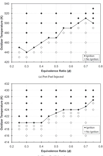
For the PFI set of simulations, a total of 47 different cases are considered by varying the preheat temperature and equivalence ratio. Figure 3.1a shows the ignition map for PFI runs with the conditions where autoignition occurs indicated by filled diamonds () and when autoignition failed indicated by unfilled diamonds ( ♦ ). Although further refinement can be made, the solid line shows the general shape of the ignition boundary. It is seen that there is a non-linear dependence of the autoignition event on these two parameters. Also, the minimum preheat temperature required for autoignition to occur increases with the increase in equivalence ratio. This can be attributed to the larger amount of ‘cooler’ fuel (at 300 K) being introduced to the mixture as theφ increases.
For the DI set, 62 cases are simulated and the ignition map showing the general shape of the boundary for the onset of autoignition is shown in Figure 3.1b. Again, a non-linear behavior is seen and the minimum preheat temperature required to ignite a richer mixture is higher. This can also be attributed to the increasing amount of ‘cooler’ fuel getting injected directly into the cylinder for higherφ values. The main difference is that the temperature range is markedly smaller than that of the PFI map. For the range of mixture fractions that have been simulated, there is an order of magnitude difference in the preheat temperature range required. Thus, direct injection looks like a better choice for combustion control since the initial temperature has to be varied only over a small range to ensure autoignition.
420 440 460 480 500 520 540
0.2 0.3 0.4 0.5 0.6 0.7 0.8
O x id ize r T e m p e ra tu re (K )
Equivalence Ratio (ϕ)
Ignition No Ignition
(a) Port Fuel Injected
414 416 418 420 422 424 426 428 430 432
0.2 0.3 0.4 0.5 0.6 0.7 0.8
O x id ize r T e m p e ra tu re (K )
Equivalence Ratio (ϕ)
Ignition
No Ignition
(b) Direct Fuel Injected