Mapping Quantitative Trait Loci by an Extension of the Haley–Knott Regression Method Using Estimating Equations

DOI: 10.1534/genetics.106.058537

Mapping Quantitative Trait Loci by an Extension of the Haley–Knott

Regression Method Using Estimating Equations

Bjarke Feenstra,*

,1

_{Ib M. Skovgaard* and Karl W. Broman}

†

*Department of Natural Sciences, Royal Veterinary and Agricultural University, DK-1871 Frederiksberg C, Denmark and†Department of Biostatistics, Johns Hopkins University, Baltimore, Maryland 21205

Manuscript received March 24, 2006 Accepted for publication May 12, 2006

ABSTRACT

The Haley–Knott (HK) regression method continues to be a popular approximation to standard interval mapping (IM) of quantitative trait loci (QTL) in experimental crosses. The HK method is favored for its dramatic reduction in computation time compared to the IM method, something that is particularly im-portant in simultaneous searches for multiple interacting QTL. While the HK method often approximates the IM method well in estimating QTL effects and in power to detect QTL, it may perform poorly if, for example, there is strong epistasis between QTL or if QTL are linked. Also, it is well known that the esti-mation of the residual variance by the HK method is biased. Here, we present an extension of the HK method that uses estimating equations based on both means and variances. For normally distributed phenotypes this estimating equation (EE) method is more efficient than the HK method. Furthermore, computer simulations show that the EE method performs well for very different genetic models and data set structures, including nonnormal phenotype distributions, nonrandom missing data patterns, varying degrees of epistasis, and varying degrees of linkage between QTL. The EE method retains key qualities of the HK method such as computational speed and robustness against nonnormal phenotype distributions, while approximating the IM method better in terms of accuracy and precision of parameter estimates and power to detect QTL.

I

N biomedical research, evolutionary biology, and agricultural science alike, it has long been of inter-est to study the genetic basis of variation in quantitative traits (such as blood pressure, litter size, or crop yield). For this purpose, experimental crosses between inbred lines are widely used; crosses of model organisms can lead to improved understanding of related human dis-eases, and crosses of inbred animal or plant species can inform breeders of important genomic regions, which may be used in breeding schemes. The genetic variance of a quantitative trait is thought to be controlled by a number of such genomic regions, or quantitative trait loci (QTL), which may interact in intricate ways (see, for example, Falconerand Mackay1996; Lynchand Walsh 1998).

With the advent of dense genetic marker maps, a lot of effort has been devoted to the development of statistical methods for locating QTL and estimating their effects. The seminal article by Lander and Botstein (1989) introduced the interval-mapping (IM) method, which considers, one at a time, a suite of putative QTL positions along the genome. In the case of a backcross, say, an

individual with genotype g¼QQor Qqat the putative QTL is assumed to have phenotype yjg N ðb_g;s2_Þ.

Since the QTL genotypes will generally not be known, the phenotype distribution given the marker data is a mixture of the two normal distributions. Closed-form expressions for the maximum-likelihood estimators are not available for mixtures of normal distributions. Thus, estimation under the IM method must be done numerically; most commonly a version of the expectation-maximization (EM) algorithm (Dempsteret al.1977) is used.

A key disadvantage to the IM method is long compu-tation time, since the EM algorithm often requires many iterations to converge. Haleyand Knott(1992) and Martı´nez _{and C}urnow (1992) independently devel-oped a simple regression method that usually approxi-mates IM very well and requires much less computation. Again, consider a backcross individual with genotype g¼QQorQqat the putative QTL. The Haley–Knott (HK) regression method applied to backcross data consists simply of regressing the individuals’ phenotypes on the conditional probabilities for having genotypesQQorQq at the putative QTL, given the marker data. In other words, an individual with marker data m is assumed to have phenotype yjm N ðb_QQPrðQQ jmÞ1PrðQqjmÞ;s2_Þ.

Since we need only to do a simple regression calculation at each putative QTL position, there are great savings in computation time compared to that of the IM method, 1_{Corresponding author:Department of Natural Sciences, Royal}

Veteri-nary and Agricultural University, Thorvaldsensvej 40, DK-1871 Frederiks-berg C, Denmark. E-mail: [email protected]

something that is particularly important when general-izing the methods for multiple-QTL models.

A number of studies have compared the IM and HK methods (Haley and Knott 1992; Xu 1998a,b; Kao 2000), and in many cases the two methods provide almost identical parameter estimates and test statistics. There are, however, important differences; for instance, it is well known that the HK method overestimates the residual variance (Xu1995; Kao2000). In general, the total genetic variance may be split into two parts, one part originating from marker genotype variation and one part from variation of QTL genotype given marker genotypes. In the HK method the latter part is con-tained in the residual variance estimate, sometimes causing overestimation of the residual variance. Also, Kao (2000), in an extensive comparison of the two methods by computer simulations, found that epistasis between QTL and linkage between QTL may lead to large differences in power to detect QTL and efficiency of parameter estimation. One further difference be-tween the IM and HK methods concerns robustness in the presence of nonnormal phenotype distributions. In such cases the IM method may produce large spu-rious LOD score peaks (Broman2003; Feenstraand Skovgaard2004), something that the HK method avoids. In this study, we develop an extension of the HK method on the basis of estimating equations. In the HK method the conditional mean of an individual’s phenotype given marker data, E(yij mi), is specified correctly, but the conditional variance Var(yi jmi) is incorrectly assumed to be constant. In the estimating equation (EE) method, we develop joint estimating equations for mean and covariance parameters, on the basis of a coherent specification of bothE(yijmi) and Var(yijmi). It has been suggested to overcome the bias of the HK method with an iteratively reweighted least-squares (IRLS) approach using Var(yijmi) to weight observations (Xu 1995, 1998a,b). The IRLS method, however, does not fully utilize information about the mean parameters contained in the conditional variance Var(yijmi) and may be expected to be less efficient than the estimating equation approach taken here.

We explore the performance of the proposed EE method on a number of real and simulated data sets, covering a range of different genetic models and data set structures. Comparison is made with the IM, HK, and IRLS methods with respect to important performance criteria, such as power, robustness, efficiency, bias, and computational speed in implementations. We focus the comparison on situations where either the HK method or the IM method is suspected to perform poorly.

GENETIC MODEL

For simplicity, we consider n individuals from a backcross population, but the results extend easily to other kinds of crosses. Consider m different QTL,

indexed by j2 f1;. . .;mg. At any given QTL, the jth say, there are two possible genotypes: QjQj and Qjqj, making the total number of possible QTL genotypes in the population 2m_{. The goal of a genetic model is to}

relate the 2m_{possible genotypic values to a set of genetic}

parameters, such that these parameters are interpret-able in terms of main and epistatic effects of themQTL. We prefer a genetic model using orthogonal contrast scales because it is consistent in the sense that the effect of a QTL is consistently defined whether the genetic model includes one, two, three, or more QTL (Kaoand Zeng2002; Zenget al.2005). The relation between the genotypic value Gi of individual i and the genetic parameters can be expressed by

Gi¼m1

Xm

j¼1 ajxij1

Xm

j,k

bjkxijxik1

Xm

j,k,l

cjklxijxikxil1

ð1Þ

with

xij¼

1

2 if homozygoteQjQj; 1

2 if heterozygoteQjqj;

m the mean genotypic value in the backcross popula-tion, ajthe main QTL effects, bjk andcjklthe two- and three-locus epistatic effects, and the dots representing fourth- and higher-order epistatic interactions. It is common to include only pairwise interactions between QTL (Kaoet al.1999; Carlborgand Andersson2002), and the genetic model is then reduced to

Gi¼m1

Xm

j¼1 ajxij1

Xm

j,k

bjkxijxik: ð2Þ

For other kinds of crosses, such as F2 populations,

different contrast scales are needed to achieve orthog-onality (Zenget al.2005).

STATISTICAL METHODS

A successful statistical model for QTL mapping should relate the phenotypes of individuals to their genotypes at the m putative QTL considered. Many authors describe this relationship using the genetic parameters mentioned above. However, we choose a different parameterization with each of the 2m _mean

yi¼Xib1ei; i¼1;. . .;n; ð3Þ

where yi is the quantitative phenotype; Xi¼ðXi1;. . .;

Xi2mÞis a row vector of length 2mindicating the

multi-locus QTL genotype;i.e., one of theXig¼1, the rest are zeros;b¼ðb₁; . . .;b₂mÞ

T

is the vector of parameters to be estimated; and ei is a random error term with an unspecified distribution. The relationship between the model parametersband the genetic model parameters is important to guide the formulation of relevant hy-potheses to test and to interpret the estimates from the final model. Fortunately, estimates of the model param-eters are readily translated to genetic parameter esti-mates; we outline how to do this below.

A key QTL-mapping problem is how to deal with missing genotype data, since the QTL genotypes,Xi, are generally not observed. A number of approaches exist for this; we briefly describe the IM and HK methods and go on to introduce the proposed EE method.

Interval mapping: The interval-mapping method, pioneered by Landerand Botstein(1989) and gener-alized to multiple loci by Kaoet al.(1999), was the first approach to fully exploit the fact that QTL are located in intervals flanked by genetic markers with observed ge-notypes. This means that given a genetic marker map and a putative QTL position and assuming a map function, we may calculate pig ¼Pr(gjmi), the condi-tional probability of QTL genotype ggiven the multi-point marker data mi. The IM method assumes that ei N ð0; s2Þ in Equation 3 and models the pheno-types given the observed marker data as a mixture of normal distributions. The likelihood function for the parameters,b,s2_is

Lðb;s2Þ ¼Y

n

i

X

g

pigfðyi;bg;s2Þ ð4Þ

with pig defined as above and f(y; bg, s2) being the density function of a normal distribution with meanbg and variances2_.

Haley–Knott regression:The Haley–Knott regression method deals differently with the missing observations Xigin the statistical model (3). Although the genotypes Xigare unobserved, we may calculate their conditional expectations given the marker data. Actually, in the case of backcross populations,E(Xigjmi)¼pig, since the Xig are indicator variables. The HK method replaces Xig with E(Xigjmi) in the regression (3), which then becomes

yi ¼EðXijmiÞb1ei; i¼1;. . .;n; ð5Þ

still assuming thatei N ð0; s2Þ. Thus, the likelihood function is

Lðb;s2Þ ¼Y

n

i

f yi;

X

g

pigbg;s2

!

; ð6Þ

which may be maximized easily by standard regression techniques.

An estimating equation method:Like the IM and HK methods, the estimating equation method considers the phenotype distribution given the marker data. Initially, we assume that the marginal density function of the phenotype,yi, given the marker data,mifor individuali has the general form

fðyijmiÞ ¼

X

g

pigfðyi j gÞ; ð7Þ

where pig is defined as before and f(yjg) is the con-ditional density function ofygiven the QTL genotypeg. We make no specific assumptions about the f(yjg), provided that these distributions have moments of at least second order. Interval mapping is a special in-stance of Equation 7 with thef(yjg) being normal dis-tributions. We now obtain the following expressions for the conditional mean and variance of the phenotypes given the marker data

EðyijmiÞ ¼mi ¼

X

g

pigbg ð8Þ

VarðyijmiÞ ¼s2i ¼E½VarðyijgÞ jmi

1Var½EðyijgÞ jmi

¼s2₁ X

g

pigb2gm2i; ð9Þ

wherebgis the mean inf(yjg). In Equation 9, we have partitioned the phenotypic variance into two compo-nents; the first component,s2_{, is assumed to be the same} for all individuals and QTL genotypes and may be interpreted as the environmental variance, whereas the second component corresponds to the variance due to uncertainty of QTL genotype given marker data and varies with marker and QTL genotype.

To estimate theb_g-parameters as well ass2_{, we must} find a set of estimating equations for the parameters sat-isfying the requirement that their expectation equals 0. For simplicity, we further make the assumption in this article that yijmi N ðmi;s2iÞ. This resembles the as-sumption in the HK method thatyijmi N ðmi;s

2_{Þ; we}

view the method presented here as an extension of the HK method that uses a coherent specification of both E(yijmi) and Var(yijmi) by which the variance reflects the uncertainty about the QTL genotype. We use the resulting score equations as estimating equations for the parameters. It should be emphasized, however, that these score equations may be used perfectly well as estimating equations without assuming normality.

The contribution of a single observation to the neg-ative log-likelihood function for the normal model is

loggðyiÞ ¼const:11₂logs2i 1

1 2

yimi si

2

:

the resulting score function equal to 0 yields the esti-mating equations

EEb_g:

X

i

pig d_ig

si

ðz2_i 1Þ1zi

si

¼0 ð10Þ

EEs2: 1 2

X

i

z2_i 1

s2_i ¼0; ð11Þ

wherezi ¼

def yimi

ð Þ=s_iandd_igdef¼ðb_gm_iÞ=s_i. Note that E(zi) ¼ 0 and E(zi2) ¼ 1, confirming that the ex-pectations of the left-hand sides of both Equations 10 and 11 equal 0 as required.

The estimating equations must be solved numerically. To do so, we implemented an algorithm that uses two conditional maximizations in each iteration. First, estimates of bg are updated by solving Equation 10 while keeping fixeds2_{and theb}

g’s that enter insiand zi2. Second, an updated estimate ofs2is obtained by solving Equation 11 with thebg’s fixed. We iterate until the estimates converge.

Relation to iteratively reweighted least-squares re-gression: Xu (1995) first pointed out that the HK method tends to give biased estimates of the residual variance. It was suggested to correct the bias by using Equations 8 and 9 for the conditional mean and variance, respectively, of the phenotypes given full marker data. Xu (1998a,b) further assumed that yijmi N ðmi;s2iÞand claimed to maximize the corsponding likelihood function by the iteratively re-weighted least-squares method. In the IRLS method, the variance is written

s2_i ¼s2vi;

where vi¼11ð1=s2ÞðPgpigb2gm 2

iÞ; i.e., vi depends both ons2_{and on the b}

g. In the iterations, updated parameter estimates are obtained by treating thevi as known weights and performing weighted least-squares regression,

˜

b¼ ðUTV1UÞ1_UT_V1_{y ð12Þ} and

˜

s2¼ 1

n2mðyUb˜Þ

T_V1_{ðyUb˜Þ; ð13Þ}

withVan3 ndiagonal matrix of the weightsvi,ythe n-vector of phenotype observations, and

U¼

p11 p1;2m

.. .

... pn1 pn;2m

0 B @

1 C

A: ð14Þ

The above two equations correspond to Equations 7 and 8 in Xu (1998b). It may be shown that IRLS

iterations using Equations 12 and 13 are (asymptoti-cally) equivalent with using

EEIRLS;bg:

X

i

pig

yimi

s2_i ¼0 ð15Þ

as an estimating equation forbgand using

EEIRLS;s2: X

i

ðyimiÞ2 s2

i

1

¼0 ð16Þ

as an estimating equation for s2_{. These estimating} equations are simpler than the ones (Equations 10 and 11) used in the EE method, and intuitively it might be expected that the EE method captures more in-formation about the parameters than the IRLS method. In theappendix, we demonstrate that the EE method is indeed more efficient than the IRLS method under the assumptions used here. Situations where the assump-tion thatyijmi N ðmi;s

2

iÞis not met are explored by computer simulation in theresults.

Estimating genetic parameters: To illustrate the translation from genetic parameters in the genetic model (1) to mean parameters in the statistical model (3) and vice versa, we consider parameters from a model with three loci in a backcross population.

At each QTL, we index homozygotes by 2 and heterozygotes by 1,e.g., the parameterb211corresponds

to QTL genotypeQ1Q1/Q2q2/Q3q3. Expressed in matrix

notation, the relation between the two types of param-eters is b₂₂₂ b₂₂₁ b₂₁₂ b₂₁₁ b₁₂₂ b₁₂₁ b₁₁₂ b₁₁₁ 0 B B B B B B B B B B B B B B B B @ 1 C C C C C C C C C C C C C C C C A ¼ 1 1 2 1 2 1 2 1 4 1 4 1 4 1 8 1 1

2 1212 14141418 1 1₂1

2 1 2 1 4 1 4 1 4 1 8 1 1 2 1 2 1 2 1 4 1 4 1 4 1 8 11

2 12 121414 14 18 11

2 1 2 1 2 1 4 1 4 1 4 1 8 11

212 12 141414 18 11

21212 14 14 1418 0 B B B B B B B B B B B B B B B B @ 1 C C C C C C C C C C C C C C C C A m a1 a2 a3 b12 b13 b23 c123 0 B B B B B B B B B B B B B B B B @ 1 C C C C C C C C C C C C C C C C A

ð17Þ

orb¼Sc, whereSis the genetic effect design matrix andcis the vector of genetic parameters. Conversely,c

may be found from bbyc ¼S1_{b. In the case where} there is no three-locus epistasis,i.e.,c123¼0, there is a

constraint on the parameter vectorbin the sense that

b111can be expressed as a function of the other seven bg’s. Writing the genetic effect design matrix as

S¼ S11 S12

S21 S22

;

whereS11is the top left 737 submatrix, we may express b111as

whereb_j7is the restriction ofbholding the first seven

parameters. Evaluating the expression yieldsb111¼b222

b221b2121b211b1221b1211b112. Obviously, for

other models and kinds of crosses different constraints onbapply. These may be found in a similar manner.

RESULTS

We explored the behavior of the IM, HK, IRLS, and EE methods over a range of real and simulated data sets. As a starting point, we considered the simple situation of detecting a single QTL and estimating its effect. A backcross population was simulated with a single QTL placed at the center of chromosome 1, which had a length of 100 cM and six evenly spaced markers. Progeny sizes of 50, 100, and 200 were considered and the corresponding ranges of additive effects of the QTL (a1in Equation 2) were 0.54–3.80, 0.34–2.00, and 0.20–

1.00, respectively. In each case, six different values for the additive effect were simulated. Moreover, three different genetic models were used in the simulation setup. First, no other QTL were segregating in the population. Second, a QTL of moderate effect (a2 ¼ 0.60) was

segregating at a position unlinked to chromosome 1. Third, two unlinked but strongly interacting QTL (a2¼

1.00, a3 ¼ 1.00, and b23 ¼ 4.00) were segregating at

positions unlinked to chromosome 1. The environmen-tal variation was sampled from a standard normal distribution in all cases. Single-locus scans were con-ducted with all four methods to detect the QTL on chromosome 1. In this simple setup there were only minor differences between the methods for all genetic models, and we therefore summarize the results in text only. Power and precision of locating the QTL were virtually the same for all methods as were mean param-eter estimates. In accordance with previous reports (Xu 1995; Kao 2000) the HK method overestimated the residual variance. There was a slight but consistent trend that the lowest standard deviations and mean squared errors on mean parameter estimates were seen with the IM method followed by the EE, IRLS, and HK methods. Since the differences in the simple simulation setup were only minor, we focus our attention in the following on more complicated situations where either the HK method or the IM method is known to perform poorly.

Nonrandom missing data patterns:In many cases the costs involved in genotyping an individual for a large collection of genetic markers are much higher than the costs of obtaining the individual’s phenotype. In such situations, selective genotyping, where individuals with extreme phenotypes are genotyped much more heavily than intermediate ones, may be an effective strategy for reducing experimental costs without losing much in-formation about the QTL behind the trait of interest (Lander and Botstein 1989; Darvasi and Soller 1992; Senet al.2005). It appears, however, that the HK

method is particularly sensitive to the special kind of nonrandom missing data that follow from selective genotyping.

Consider, for example, the data set consisting of 250 backcross mice studied for hypertension in Sugiyama et al.(2001). Initially, individuals with extreme pheno-types were genotyped; in regions showing evidence for QTL, all individuals were genotyped and additional markers were added. Further, at some markers only recombinant individuals were genotyped. In 8 of the 19 autosomes, only 46 individuals in each extreme of the phenotype distribution were genotyped;i.e., the middle 158 individuals were not genotyped for any markers on those chromosomes. When those eight chromosomes are scanned with both the IM and the HK methods, the LOD curves produced by the HK method exceed those produced by the IM method, with differences of up to 1 LOD score unit. If, however, the phenotypes of in-termediate individuals are discarded, the LOD curves produced by the HK method are virtually indistinguish-able from those produced by the IM method for the eight chromosomes considered (results not shown).

To further investigate this behavior of the HK method, we simulated 250 backcross individuals and a single chromosome of length 100 cM with 10 markers and a QTL at position 45 cM explaining 14% of the phenotypic variance. We scanned the simulated chro-mosome with one-locus versions of the IM, HK, and EE methods in the case where all individuals had complete marker data, but we also considered the case of selective genotyping by letting observations from the 40th to the 60th percentile in phenotype distribution have missing observations for all markers on the chromosome.

Figure 1 shows that discarding marker genotypes for individuals in the middle 20% of the phenotype distribution inflates the HK LOD curve over the whole range of the chromosome compared to using the HK method with all marker data and compared to using the IM method. The inflation is most pronounced at the peak of the LOD curve. The EE method almost completely avoids this problem of inflated LOD curves. In Figure 1, it can be seen that the LOD curves for the EE method are close to the IM curve, both in the case of full marker data and in the case of selective genotyping. A closer look at the HK method explains the phenomenon of inflated LOD curves. The one-locus regression may be written

yi ¼bQq1ðbQQbQqÞPrðQQjmiÞ1ei;

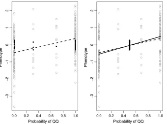
where ei N ð0;s2Þ. In Figure 2, regression lines are shown for the position with the largest LOD score. Observations from the middle 20% of individuals are shown as solid dots and other observations as open circles.

horizontal. In Figure 2, right, the middle 20% of individuals have missing marker data. Thus, there is no marker information for those individuals about Pr(QQjmi) and this probability therefore equals 0.5. Consequently, the points corresponding to the middle 20% of individuals are translocated horizontally to Pr(QQjmi)¼0.5, thereby removing positive residuals from the low end of the regression line and negative residuals from the high end, causing the line to become steeper. Furthermore, the points cluster closer around the regression line with selective genotyping, meaning

that the likelihood under the alternative is larger. It is, however, unchanged under the null hypothesis of no QTL effect, since the points do not move vertically, and the LOD score is thereby inflated. Also, the steeper slope of the regression line means that the size of the QTL effect is overestimated by the HK method in the case of selective genotyping.

As may be seen from the simulation example in Figure 1, the EE method almost completely avoids this problem, as it weights observations by their inverse variances. Thus, observations with large variance due to

Figure 2.—Haley–Knott regression

lines at the position with largest LOD score in a simulated data set. Lines are shown in the case of full marker data (left side, dashed line) and in the case of selective genotyping with missing marker data for the intermediate 20% of individuals (right side, solid line). Figure1.—A simulation example of QTL mapping with a population of 250 backcross individuals and a single QTL at 45 cM.

uncertainty of QTL genotype [i.e., Pr(QQjmi) close to 0.5] have little weight in the likelihood calculation.

Nonnormal phenotype distributions:In earlier work, we have considered QTL mapping strategies in situa-tions where the phenotype distribution deviates from a normal distribution (Broman 2003; Feenstra and Skovgaard 2004). The IM method can occasionally produce spurious LOD score peaks in regions of low genotypic information (e.g., widely spaced markers), especially if the phenotype distribution deviates mark-edly from a normal distribution. This is caused by the fact that the IM method models the phenotype distri-bution as a mixture of two or more normal distridistri-butions when a QTL is included in the model, while only using a single normal distribution under the null hypothesis. If the phenotype distribution is not normal, the model including a QTL may fit the data much better than the null model, even if there is no real QTL and no genetic marker information (Feenstraand Skovgaard2004). In Feenstraand Skovgaard(2004), we considered models with a single QTL and developed a two-component mixture model that avoids the problem of spurious LOD score peaks. Here, we broaden our view to models with more than one QTL with possible epistatic inter-actions between loci. It appears that the problem of spurious LOD score peaks gets worse when the IM method is used to map more QTL simultaneously.

Figure 3 shows the results of two-QTL scans of a simulated data set consisting of 80 backcross individu-als, five chromosomes of length 140 cM with 12, 12, 8, 6, and 4 markers, respectively, and two epistatically inter-acting QTL on chromosome 1 at position 45 cM and chromosome 2 at position 5 cM, respectively. In Figure 3A, results for the IM method are shown. It can be seen that the interacting QTL on chromosomes 1 and 2 are detected with high LOD scores. However, there are also large areas in the plot corresponding to combinations of positions on other chromosomes with high LOD scores. These high LOD score areas involve chromo-somes with few markers,i.e., little genetic information, strongly suggesting that this is the same kind of artifact as the spurious LOD score peaks seen in one-QTL scans. In this simulation example, the residual variation was normal, but the influence of the two interacting QTL caused the phenotype distribution to be nonnormal, thereby allowing the phenomenon of artificially high LOD scores at other positions.

The HK method is known to be quite robust toward nonnormal phenotype distributions (Rebaı¨1997), and both the HK and the EE methods are immune to the artifact of spurious LOD score peaks, since single nor-mal distributions are used both when one or more QTL are included in the model and under the null hypoth-esis of no QTL effect. Figure 3B shows LOD scores for a two-QTL scan of the same data set by the EE method. The interacting QTL on chromosomes 1 and 2 are de-tected, but no other combinations of positions show

high LOD scores. The HK method gave very similar re-sults to the EE method for these data (rere-sults not shown).

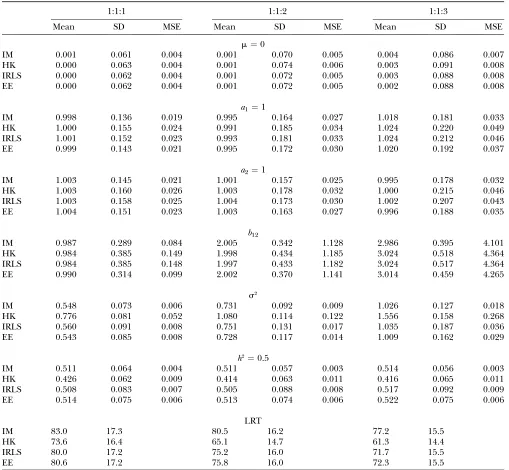
Epistasis between QTL:In an extensive analytical and simulation-based comparison between the IM and HK methods, Kao (2000) found that there may be signifi-cant differences between the two methods, especially if QTL interact or are linked. Here, we focus on the situa-tion where two unlinked QTL interact. We use the simula-tion setup from Table 3 in Kao(2000) and also include Figure_{3.—LOD scores for a two-dimensional, two-QTL}

the IRLS and EE methods in the comparison. Data were generated from a genetic model with two unlinked epi-static QTL with genetic parametersm¼0,a1¼1,a2¼1,

andb12¼1, 2, or 3 (cf.Equation 1). Thus, the strength of

epistasis was increased compared to the additive effects of the QTL. Estimates of the genetic parameters,s2_{, and} the broad sense heritability, h2 _{(see, for example,} Falconer and Mackay 1996), were recorded as well as likelihood-ratio test (LRT) statistics comparing the full model with a null model of no QTL.

Table 1 displays the simulation results. The means of the estimated main and epistatic effects by the four methods are almost identical and very close to the true values for all three degrees of epistasis. Standard deviations (SDs) and mean square errors (MSEs) are smallest for the IM method, slightly larger for the EE method, and largest for the HK method. The IRLS method resembles the HK method with respect to SDs and MSEs for the main and epistatic effect estimates.

TABLE 1

Comparison of the IM, HK, IRLS, and EE methods applied to simulated data under different strengths of epistasis

1:1:1 1:1:2 1:1:3

Mean SD MSE Mean SD MSE Mean SD MSE

m¼0

IM 0.001 0.061 0.004 0.001 0.070 0.005 0.004 0.086 0.007 HK 0.000 0.063 0.004 0.001 0.074 0.006 0.003 0.091 0.008 IRLS 0.000 0.062 0.004 0.001 0.072 0.005 0.003 0.088 0.008 EE 0.000 0.062 0.004 0.001 0.072 0.005 0.002 0.088 0.008

a1¼1

IM 0.998 0.136 0.019 0.995 0.164 0.027 1.018 0.181 0.033 HK 1.000 0.155 0.024 0.991 0.185 0.034 1.024 0.220 0.049 IRLS 1.001 0.152 0.023 0.993 0.181 0.033 1.024 0.212 0.046 EE 0.999 0.143 0.021 0.995 0.172 0.030 1.020 0.192 0.037

a2¼1

IM 1.003 0.145 0.021 1.001 0.157 0.025 0.995 0.178 0.032 HK 1.003 0.160 0.026 1.003 0.178 0.032 1.000 0.215 0.046 IRLS 1.003 0.158 0.025 1.004 0.173 0.030 1.002 0.207 0.043 EE 1.004 0.151 0.023 1.003 0.163 0.027 0.996 0.188 0.035

b12

IM 0.987 0.289 0.084 2.005 0.342 1.128 2.986 0.395 4.101 HK 0.984 0.385 0.149 1.998 0.434 1.185 3.024 0.518 4.364 IRLS 0.984 0.385 0.148 1.997 0.433 1.182 3.024 0.517 4.364 EE 0.990 0.314 0.099 2.002 0.370 1.141 3.014 0.459 4.265

s2

IM 0.548 0.073 0.006 0.731 0.092 0.009 1.026 0.127 0.018 HK 0.776 0.081 0.052 1.080 0.114 0.122 1.556 0.158 0.268 IRLS 0.560 0.091 0.008 0.751 0.131 0.017 1.035 0.187 0.036 EE 0.543 0.085 0.008 0.728 0.117 0.014 1.009 0.162 0.029

h2_¼0.5

IM 0.511 0.064 0.004 0.511 0.057 0.003 0.514 0.056 0.003 HK 0.426 0.062 0.009 0.414 0.063 0.011 0.416 0.065 0.011 IRLS 0.508 0.083 0.007 0.505 0.088 0.008 0.517 0.092 0.009 EE 0.514 0.075 0.006 0.513 0.074 0.006 0.522 0.075 0.006

LRT

IM 83.0 17.3 80.5 16.2 77.2 15.5

HK 73.6 16.4 65.1 14.7 61.3 14.4

IRLS 80.0 17.2 75.2 16.0 71.7 15.5

EE 80.6 17.2 75.8 16.0 72.3 15.5

As in Kao(2000), we find that the most conspicuous difference between the IM and HK methods is the bias of the HK method in the estimation ofs2_andh2_{. The EE} method does not show this bias and provides almost identical estimates of s2 _{and h}2 _{to those by the IM} method (Table 1). The IRLS method also performs very well in this respect.

We note that the results are in good accordance with those from Kao(2000), with one exception. When cal-culating the genetic variance component, and thereby the heritability for the HK method, Kao (2000) does not use the model that the data were simulated from (Equation 3). Rather, it appears that the modified re-gression model (Equation 5) is used for calculating the genetic variance. Indeed, when calculating the genetic variance on the basis of Equation 5 we geth2_-estimates for the HK method of 0.310, 0.279, and 0.259 for the three levels of epistasis, which are very close to the values 0.302, 0.277, and 0.255 reported by Kao(2000). Thus, while our estimates of h2 _{by the HK method are also} clearly biased (Table 1), our findings indicate that the bias in Kao(2000) is exaggerated. In any case, the EE method avoids the bias and approximates the IM method very well for all parameter estimates and with respect to the LRT statistics. In addition, it is superior to the IRLS method, considering the efficiency of the parameter estimates.

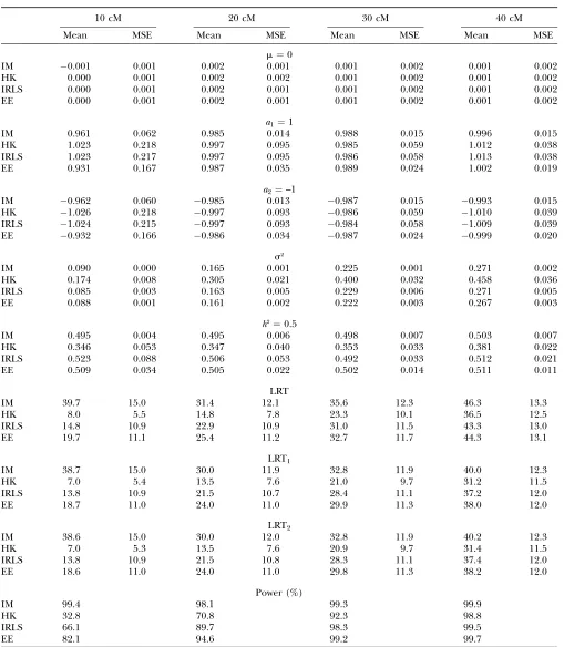
Linked QTL: The most pronounced differences between the IM and HK methods are found when two QTL of opposite effect are linked (Kao2000). Here we focus on that situation, using the simulation setup from Table 5 in Kao (2000) and also including the EE and IRLS methods in the comparison. Data were generated from a genetic model with two linked QTL of opposite effects without epistasis (m¼0,a1¼1,a2¼ 1,b12¼0,

cf. Equation 1). The two QTL were placed in two neighboring 40-cM intervals and were 10, 20, 30, or 40 cM apart from each other. Haldane’s map function was used.

Table 2 shows the simulation results. Again, the means of the estimates ofm,a1, anda2are close to the

true values for all four methods, and again the IM method has the lowest MSEs on the paramater esti-mates, followed by the EE method and then the IRLS and HK methods. Estimates ofs2_andh2_{from the HK} method are even more biased than in the epistasis case. Again, the IM, IRLS, and EE methods provide very similar estimates ofs2_andh2_{. Like in the epistasis} sim-ulations, the results are in good accordance with those reported in Kao (2000) with the exception that the h2_{-estimates for the HK method are not as dramatically} biased as those in Kao(2000).

As for the power to detect two QTL, the EE method provides higher LRT statistics and greater power com-pared to the HK and IRLS methods. When the two QTL are.20 cM apart, the LRT statistics and power results are similar for the IM and EE methods. However, for

QTL only 10 cM apart, the LRT statistics from the IM method are more than twice as large as those from the EE method, three times larger than the IRLS statistics, and five or six times larger than those from the HK method (Table 2). This is related to the phenomenon of spurious LOD score peaks that the IM method occa-sionally shows with nonnormal phenotype distributions. The residual variance used for the simulations when the QTL were only 10 cM apart was small (0.091) compared to the additive effects. This means that phenotype distributions resulting from the simulations bore much closer resemblance to a mixture of three normal distributions (with means 1, 0, and 1 as given by the two-locus additive model) than to one with two normals (corresponding to a one-locus model). Indeed, the two additive QTL were detected with high LRT statistics and high power.

However, this did not come without a price. To investigate the effect on chromosomes unlinked to QTL we simulated a second chromosome with the same marker spacing, but with no QTL on it, while retaining the phenotypes (which are strongly influenced by the QTL on chromosome 1). We then considered positions on this second chromosome that mirrored the positions of the QTL on the first chromosome and calculated LRT statistics for going from a model with two additively acting QTL on the second chromosome to a model with just one QTL (data not shown). Since there were no QTL on this second chromosome, we would expect low LRT statistics. On the contrary, very high LRT statistics were observed for the IM method (the 95th percentile was at 35.5), strongly suggesting that the phenomenon of spurious LOD score peaks had occurred. The HK, IRLS, and EE methods did not show such high LRT statistics on the unlinked chromosome (the 95th percentiles were at 4.2, 6.0, and 3.8, respectively).

Taking a closer look at the LRT statistics for the IRLS method on this second chromosome with no QTL on it revealed another problem. Following Xu (1998a,b) we calculate LRT statistics for the IRLS method using the likelihood based on the assumption that yijmi

N ðm_i;s2

iÞ. However, it follows from theappendixthat the IRLS method does not give maximum-likelihood estimates corresponding to this likelihood (in contrast to the EE method). Thus, the LRT statistics for the IRLS method are not guaranteed to be nonnegative. In fact, analyzing the second chromosome with no QTL while keeping the phenotypes, which are influenced by the two 10-cM-apart QTL on the first chromosome, yielded negative LRT statistics for the IRLS method in400 of 1000 simulation replicates with the 10th percentile being at1.2.

TABLE 2

Comparison of the IM, HK, IRLS, and EE methods applied to simulated data under different strengths of linkage

10 cM 20 cM 30 cM 40 cM

Mean MSE Mean MSE Mean MSE Mean MSE

m¼0

IM 0.001 0.001 0.002 0.001 0.001 0.002 0.001 0.002

HK 0.000 0.001 0.002 0.002 0.001 0.002 0.001 0.002

IRLS 0.000 0.001 0.002 0.001 0.001 0.002 0.001 0.002

EE 0.000 0.001 0.002 0.001 0.001 0.002 0.001 0.002

a1¼1

IM 0.961 0.062 0.985 0.014 0.988 0.015 0.996 0.015

HK 1.023 0.218 0.997 0.095 0.985 0.059 1.012 0.038

IRLS 1.023 0.217 0.997 0.095 0.986 0.058 1.013 0.038

EE 0.931 0.167 0.987 0.035 0.989 0.024 1.002 0.019

a2¼–1

IM 0.962 0.060 0.985 0.013 0.987 0.015 0.993 0.015 HK 1.026 0.218 0.997 0.093 0.986 0.059 1.010 0.039 IRLS 1.024 0.215 0.997 0.093 0.984 0.058 1.009 0.039 EE 0.932 0.166 0.986 0.034 0.987 0.024 0.999 0.020

s2

IM 0.090 0.000 0.165 0.001 0.225 0.001 0.271 0.002

HK 0.174 0.008 0.305 0.021 0.400 0.032 0.458 0.036

IRLS 0.085 0.003 0.163 0.005 0.229 0.006 0.271 0.005

EE 0.088 0.001 0.161 0.002 0.222 0.003 0.267 0.003

h2_¼0.5

IM 0.495 0.004 0.495 0.006 0.498 0.007 0.503 0.007

HK 0.346 0.053 0.347 0.040 0.353 0.033 0.381 0.022

IRLS 0.523 0.088 0.506 0.053 0.492 0.033 0.512 0.021

EE 0.509 0.034 0.505 0.022 0.502 0.014 0.511 0.011

LRT

IM 39.7 15.0 31.4 12.1 35.6 12.3 46.3 13.3

HK 8.0 5.5 14.8 7.8 23.3 10.1 36.5 12.5

IRLS 14.8 10.9 22.9 10.9 31.0 11.5 43.3 13.0

EE 19.7 11.1 25.4 11.2 32.7 11.7 44.3 13.1

LRT1

IM 38.7 15.0 30.0 11.9 32.8 11.9 40.0 12.3

HK 7.0 5.4 13.5 7.6 21.0 9.7 31.2 11.5

IRLS 13.8 10.9 21.5 10.7 28.4 11.1 37.2 12.0

EE 18.7 11.0 24.0 11.0 29.9 11.3 38.0 12.0

LRT2

IM 38.6 15.0 30.0 12.0 32.8 11.9 40.2 12.3

HK 7.0 5.3 13.5 7.6 20.9 9.7 31.4 11.5

IRLS 13.8 10.9 21.5 10.8 28.3 11.1 37.4 12.0

EE 18.6 11.0 24.0 11.0 29.8 11.3 38.2 12.0

Power (%)

IM 99.4 98.1 99.3 99.9

HK 32.8 70.8 92.3 98.8

IRLS 66.1 89.7 98.3 99.5

EE 82.1 94.6 99.2 99.7

method, and also avoids problems with artificially high LRT statistics on other chromosomes observed with the IM method and negative LRT statistics seen with the IRLS method.

DISCUSSION

Most quantitative traits are believed to be influenced by multiple QTL that may interact, and it is therefore desirable to model the effect of these QTL simulta-neously. This may, however, pose a formidable compu-tational burden even for a moderate number of loci, since the number of possible models increases expo-nentially with the number of loci considered in the model. These computational problems may be ad-dressed along two main lines of attack.

First, the multidimensional model space may be searched much more efficiently compared to doing an exhaustive grid search. More efficient model search pro-cedures include techniques such as forward selection and backward elimination to search through nested sequences of models (Broman and Speed 2002), randomization algorithms such as Markov chain Monte Carlo (Yi2004) or a genetic algorithm (Carlborget al. 2000), and deterministic global optimization algo-rithms that repetitively divide the search space into smaller parts (Ljungberget al.2004).

Second, any model space search procedure will involve fitting the statistical model many times. Thus, a fast and efficient method for estimating model parameters is needed to reduce total computation time. Currently, the HK method is preferred as a fast approximation to the IM method for estimating model parameters. However, the HK method is known to produce biased estimates of the residual variance and to be sensitive to epistasis and linkage between QTL.

We have focused on the latter issue, fitting multilocus QTL models fast and efficiently. An extension of the HK method is proposed and formulated using estimating equations. This EE method involves simultaneously solving estimating equations for both mean and vari-ance parameters. We have compared the IM, HK, IRLS, and EE methods primarily by computer simulation, focusing on situations where either the HK method or the IM method performs poorly.

It is found here that the HK method is sensitive to certain missing data patterns,e.g., as arise from selective genotyping. With such data, the HK LOD curve may be artificially inflated over large stretches of the genome. The EE method alleviates this problem and produces LOD curves very similar to IM LOD curves. Also, the HK method suffers from large bias in the estimation of the residual variance and has lower power to detect QTL than the IM method, especially in situations of epistati-cally interacting QTL or QTL that are linked (Kao 2000). Here, it is found that the EE method approx-imates the IM method more closely in cases of epistasis

or linked QTL: it produces unbiased estimates of the residual variance, it has smaller standard deviations on the parameter estimates than the HK method, and it has high power to detect even closely linked QTL of opposite effect.

In comparison to the IM method, the EE method has increased robustness toward nonnormal phenotype dis-tributions. The IM method occasionally produces large spurious LOD score peaks in regions with little marker information if the phenotype distribution deviates markedly from a normal distribution (Feenstra and Skovgaard2004). This artifact is caused by the fact that a mixture distribution with many components always produces a better fit than a mixture with few compo-nents. It is found that the problem is aggravated for models with multiple loci. The HK and EE methods are immune to this problem, since single normal distribu-tions are used both for full and for reduced models.

The EE method is not as fast as the HK method, since it involves solving a set of estimating equations numer-ically. Still, it may provide gains in computational speed compared to the IM method. In full two-locus genome scans, for example, our implementation of the EE method was twice as fast as the IM method in compu-tation time, and we expect additional gains in speed when the code has been further optimized.

We have demonstrated analytically in the appendix that the EE method is more efficient than the HK and IRLS methods under the assumption that yijmi

N ðm_i;s2

iÞ. Admittedly, this assumption may often be violated; the residual variation of certain traits may be inherently nonnormal and the effects of major QTL may also cause the phenotype distribution to deviate from normality. It is evident, however, from the simu-lations investigating epistasis and linkage that the EE method can also be very efficient compared to the HK and IRLS methods in cases where yijmiis clearly not normally distributed. Moreover, the IRLS method may result in negative LRT statistics, something that the EE method avoids.

The estimating equations used by the EE method involve weighted linear combinations of the simple esti-mating functionsyimiand (yimiÞ

2_=s2

i 1. Under the assumption taken by the HK, EE, and IRLS methods that yijmi N ðmi;s2iÞ, it may be shown that the EE method is asymptotically optimal in the sense that any other linear combination of the simple estimating functions gives rise to estimates with a larger asymptotic covariance matrix (Godambe and Heyde 1987). A further development might be to assume a specific distribution of the residuals in Equation 3 and derive optimally weighted combinations of the simple estimating functions on the basis of this distribution. We anticipate that the gain in efficiency compared to the EE method will be minimal and possibly at the expense of greater numerical instability.

Whittaker (2001) provide a recent exception and develop a generalized estimating equation (GEE) ap-proach for QTL mapping of multiple correlated traits. However, in contrast to the EE method, these authors assume that the variance due to uncertainty of QTL genotype given marker genotype could be ignored. This is the same assumption taken by the HK method, which may lead to problems of inflated LOD curves, biased variance estimates, and low power, as seen here. It might be worthwhile to pursue the estimating equation approach further compared to this presentation. For instance, the EE method, as proposed here, tests hypotheses by likelihood-ratio tests based on a normal model. It would, however, be perfectly possible to still obtain parameter estimates by solving the estimating equations (Equations 10 and 11), but then use, e.g., score-type test statistics for hypothesis testing. This could possibly contribute some extra robustness com-pared to using the EE method in conjunction with LRT statistics.

In conclusion, the estimating equation method pre-sented here may be used as a fast and efficient approach for mapping multiple QTL. Generally, it performs better than the HK method at approximating the IM method. Importantly, it avoids problems shown by the HK method in situations with special missing data patterns, epistasis, and linked QTL. Furthermore, the EE method is more robust than the IM method toward nonnormal phenotype distributions, and it is computa-tionally faster. These issues become especially important in the analysis of multiple-QTL models.

The EE method was implemented with new functions soon to be incorporated in the QTL mapping software R/qtl (Bromanet al.2003), an add-on package for the general statistical software, R (Ihakaand Gentleman 1996; R DevelopmentCoreTeam2005).

We are grateful to three anonymous reviewers for their constructive comments on an earlier version of this manuscript. This work was supported in part by a grant from Christian and Ottilia Brorson’s Fund (to B.F.), as well as by National Institutes of Health research grant R01 GM074244 (to K.W.B.).

LITERATURE CITED

Broman, K. W., 2003 Mapping quantitative trait loci in the case of a

spike in the phenotype distribution. Genetics163:1169–1175. Broman, K. W., and T. P. Speed, 2002 A model selection approach

for the identification of quantitative trait loci in experimental crosses. J. R. Stat. Soc. B64:641–656.

Broman_{, K. W., H. W}u_,S´_{. S}en_{and G. A. C}hurchill_{, 2003 R/qtl:}

QTL mapping in experimental crosses. Bioinformatics19:889–890. Carlborg_, O¨_{., and L. A}ndersson_{, 2002 Use of randomization}

testing to detect multiple epistatic QTLs. Genet. Res.79:175–184.

Carlborg,O¨_{., L. A}nderssonand B. Kringhorn, 2000 The use of a

genetic algorithm for simultaneous mapping of multiple inter-acting quantitative trait loci. Genetics155:2003–2010. Darvasi_{, A., and M. S}oller_{, 1992 Selective genotyping for}

determi-nation of linkage between a marker locus and a quantitative trait locus. Theor. Appl. Genet.85:353–359.

Dempster, A. P., N. M. LairdandD.B.Rubin, 1977 Maximumlikelihood

from incomplete data via the EM algorithm. J. R. Stat. Soc. B39:1–38. Falconer_{, D. F., and T. F. C. M}ackay_{, 1996 Introduction to}

Quantita-tive Genetics, Ed. 4. Pearson Education, Harlow, UK.

Feenstra_{, B., and I. M. S}kovgaard_{, 2004 A quantitative trait locus}

mixture model that avoids spurious lod score peaks. Genetics 167:959–965.

Godambe, V. P., and C. C. Heyde, 1987 Quasi-likelihood and

opti-mal estimation. Int. Stat. Rev.55:231–244.

Haley, C. S., and S. A. Knott, 1992 A simple regression method for

mapping quantitative trait loci in line crosses using flanking markers. Heredity69:315–324.

Ihaka, R., and R. Gentleman, 1996 R: a language for data analysis

and graphics. J. Comp. Graph. Stat.5:299–314.

Kao, C.-H., 2000 On the differences between maximum likelihood

and regression interval mapping in the analysis of quantitative trait loci. Genetics156:855–865.

Kao_{, C.-H., and Z-B. Z}eng_{, 2002 Modeling epistasis of quantitative}

trait loci using Cockerham’s model. Genetics160:1243–1261. Kao_{, C.-H., Z-B. Z}eng_{and R. D. T}easdale_{, 1999 Multiple interval}

mapping for quantitative trait loci. Genetics152:1203–1216. Lander, E. S., and D. Botstein, 1989 Mapping Mendelian factors

underlying quantitative traits using RFLP linkage maps. Genetics 121:185–199.

Lange_{, C., and J. C. W}hittaker_{, 2001 Mapping quantitative trait loci}

using generalized estimating equations. Genetics159:1325–1337. Ljungberg_{, K., S. H}olmgren_andO¨_{. C}arlborg_{, 2004 Simultaneous}

search for multiple QTL using the global optimization algorithm DIRECT. Bioinformatics20:1887–1895.

Lynch, M., and B. Walsh, 1998 Genetics and Analysis of Quantitative

Traits.Sinauer, Sunderland, MA.

Marshall, A. W., and I. Olkin, 1990 Matrix versions of the Cauchy and

Kantorovich inequalities. Aequationes Mathematicae40:89–93. Martı´nez_{, O., and R. N. C}urnow_{, 1992 Estimating the locations}

and the sizes of the effects of quantitative trait loci using flanking markers. Theor. Appl. Genet.85:480–488.

R DevelopmentCoreTeam, 2005 R: A Language and Environment for

Statistical Computing. R Foundation for Statistical Computing,

Vienna.

Rebaı¨_{, A., 1997 Comparison of methods for regression interval}

map-ping in QTL analysis with non-normal traits. Genet. Res.69:69–74. Sen,S´., J. M. Satagopanand G. A. Churchill, 2005 Quantitative

trait locus study design from an information perspective. Genetics 170:447–464.

Sugiyama_{, F., G. A. C}hurchill_{, D. C. H}iggins_{, C. J}ohns_{, K. P.}

Makaritsiset al., 2001 Concordance of murine quantitative

trait loci for salt-induced hypertension with rat and human loci. Genomics71:70–77.

Xu_{, S., 1995 A comment on the simple regression method for}

inter-val mapping. Genetics141:1657–1659.

Xu_{, S., 1998a Further investigation on the regression method of}

mapping quantitative trait loci. Heredity80:364–373.

Xu, S., 1998b Iteratively reweighted least squares mapping of

quan-titative trait loci. Behav. Genet.28:341–355.

Yi, N., 2004 A unified Markov chain Monte Carlo framework

for mapping multiple quantitative trait loci. Genetics167:967– 975.

Zeng_{, Z-B., T. W}ang _{and W. Z}ou_{, 2005 Modeling quantitative}

trait loci and interpretation of models. Genetics169:1711–1725.

Communicating editor: C. Haley

APPENDIX

To demonstrate that the EE method yields more efficient estimates of the mean parameters, b, than the IRLS method, we take a closer look at the estimating equations. We letGEE(y;u) denote the 2m11 vector of estimating

10 and 11). Similarly,GIRLS(y;u) denotes the estimating functions for the IRLS method, corresponding to the

left-hand sides of Equations 15 and 16.

In general, the asymptotic distribution of an estimator ˆuthat solves a set of estimating equations G(y;u)¼0is Gaussian with meanuand variance of the so-calledsandwichform

VarðuˆÞ ¼ Eu

@Gðy;uÞ

@u

1

ðVaruðGðy;uÞÞÞ Eu

@Gðy;uÞ

@u

T

1

:

The information matrix may be found by inverting VarðuˆÞ:

iðuÞ ¼ Eu

@Gðy;uÞ

@u

T

ðVaruðGðy;uÞÞÞ1 Eu

@Gðy;uÞ

@u

:

Assuming thatyijmi N ðmi;s2iÞ(or slightly more generally, that the third and fourth cumulants are zero) the information matrices for the EE and IRLS methods are given by the matrix expressions (derivations not shown)

iEEðuÞ ¼1 2

2MMT1KKT KLT LKT LLT

ðA1Þ

iIRLSðuÞ ¼1 2

2MMT11

nðK1nÞð1

T

nKTÞ 1nðK1nÞðL1nÞ

1

nðL1nÞð1

T

nKTÞ 1nðL1nÞðL1nÞ

!

; ðA2Þ

where

M¼ 1

s₁ @m₁

@b₁

1

s_n @m_n @b₁

.. .

... 1

s₁ @m₁ @b₂m

1

s_n @m_n @b₂m

0 B B B B B B @ 1 C C C C C C A

and K¼ 1

s2₁ @s2₁

@b₁

1

s2_n @s2_n @b₁

.. .

... 1

s2₁ @s2

1

@b₂m

1

s2_n @s2

n @b₂m

0 B B B B B B B @ 1 C C C C C C C A

(i.e., 2m_{3nmatrices), andL¼ 1=s}2

1 . . . 1=s2n

(i.e., a 13nmatrix), and1nis the identity vector of lengthn. To invert the information matrices, we use the following result about inverting a partitioned square matrix. Let

A¼ A11 A12

A21 A22

;

then

A1 ¼ ðA11A12A 1

22A21Þ1 A111A12ðA22A21A111A12Þ1 ðA22A21A111A12Þ

1_A

21A111 ðA22A21A111A12Þ 1

!

:

The submatrix corresponding to A11 A12A221A21 may be considered the effective information about the mean

parameters,b, since inverting it yields the asymptotic variance on the estimate ofb. The effective information matrices for the EE and IRLS methods are

ieffEE ¼MM T₁1

2KK T1

2KL

T_ðLLT_Þ1_LKT _ðA3Þ

ieffIRLS ¼MM T₁ 1

2nðK1nÞð1

T

nKTÞ 21nK1nðL1nÞnðL1nÞ

1_ðL1

nÞ1 1_nðL1nÞ1TnKT:

¼MMT ðA4Þ

Consider the difference between the effective information for the two methods:

Dieff ¼ieffEEieffIRLS ¼ 1 2KK

T1 2KL

T_ðLLT_Þ1_LKT_:

We also consider efficiency under the HK method. The closed-form expression for the estimator ofbis

ˆ

b_HK ¼ ðUTUÞ1_UT_y withUdefined as in Equation 14. The variance of the estimator is

Varðbˆ_HKÞ ¼ ðUTUÞ1_UT_VarðyÞUðUT_UÞ1_:

The corresponding effective information aboutb may be found by inverting this matrix, since the estimator ofb

is independent of that ofs2_{under HK regression. This matrix may be written}

ieffHK ¼MN

T_ðNNT_Þ1_NMT withMas previously defined and

N¼

s1

@m₁

@b₁ sn

@m_n @b₁

.. .

...

s1

@m₁

@b_q1 sn

@m_n @b_q1

0 B B B B B B @

1 C C C C C C A

:

Consider now the difference between the effective information for the IRLS method and that for the HK method

ieffIRLSieffHK ¼MM

T_MNT_ðNNT_Þ1_NMT_:

Again, it follows from the matrix version of the Cauchy–Schwarz inequality Marshall and Olkin (1990) that