A NEAT Approach to Malware Classification

(1)

San Jose State University San Jose State University

SJSU ScholarWorks

Master's Projects Master's Theses and Graduate Research Fall 12-29-2020

A NEAT Approach to Malware Classification

Jason Do

San Jose State University

Follow this and additional works at: https://scholarworks.sjsu.edu/etd_projects

Part of the Artificial Intelligence and Robotics Commons, and the Information Security Commons Recommended Citation

Recommended Citation

Do, Jason, "A NEAT Approach to Malware Classification" (2020). Master's Projects. 973. https://scholarworks.sjsu.edu/etd_projects/973

(2)

A NEAT Approach to Malware Classification

A Project Presented to

The Faculty of the Department of Computer Science San José State University

In Partial Fulfillment

of the Requirements for the Degree Master of Science

by Jason Do December 2020

(3)

(4)

The Designated Project Committee Approves the Project Titled A NEAT Approach to Malware Classification

by Jason Do

APPROVED FOR THE DEPARTMENT OF COMPUTER SCIENCE SAN JOSÉ STATE UNIVERSITY

December 2020

Mark Stamp Department of Computer Science Rula Khayrallah Department of Computer Science Thomas Austin Department of Computer Science

(5)

ABSTRACT

A NEAT Approach to Malware Classification by Jason Do

Current malware detection software often relies on machine learning, which is seen as an improvement over signature-based techniques. Problems with a machine learning based approach can arise when malware writers modify their code with the intent to evade detection. This leads to a cat and mouse situation where new models must constantly be trained to detect new malware variants. In this research, we experiment with genetic algorithms as a means of evolving machine learning models to detect malware. Genetic algorithms, which simulate natural selection, provide a way for models to adapt to continuous changes in a malware families, and thereby improve detection rates. Specifically, we use the Neuro-Evolution of Augmenting Topologies (NEAT) algorithm to optimize machine learning classifiers based on decision trees and neural networks. We compare the performance of our NEAT approach to standard models, including random forest and support vector machines.

(6)

ACKNOWLEDGMENTS

I would like to thank my advisor, Mark Stamp, for guiding me and urging me to always try harder. This year has been riddled with obstacles, but he was always there to push me forward. His patience and compassion has kept me on the goal, and for that, I am truly grateful.

I would like to thank my committee members, Thomas Austin and Rula Khayral-lah, for their time and feedback.

I am thankful for my friends and family for being my light through many long days and sleepless nights.

Finally, I would like to thank all the professors and mentors who paved the way for my intellectual journey and my future endeavors.

(7)

TABLE OF CONTENTS

CHAPTER

1 Introduction . . . 1

2 Background . . . 3

2.1 Base Models for Comparison . . . 4

2.1.1 Decision Trees . . . 4

2.1.2 Random Forest . . . 4

2.1.3 Support Vector Machines . . . 4

2.2 Genetic Algorithms . . . 5 2.2.1 Fitness . . . 6 2.2.2 Speciation . . . 6 2.2.3 Crossover . . . 7 2.2.4 Mutation . . . 7 2.2.5 Behavior . . . 7 2.3 Previous Work . . . 8

2.4 Neuro-Evolution of Augmenting Topologies . . . 9

3 Methodology . . . 12

3.1 Feature Extraction . . . 12

3.2 Proposed Experiments . . . 12

3.3 Machine Learning Pipeline . . . 12

3.3.1 Feature Selection . . . 13

(8)

3.3.3 Classification and Evaluation . . . 13

4 Implementation. . . 14

4.1 Dataset and Malware Families . . . 14

4.2 Programming Specifications . . . 15

4.3 Experimental Design . . . 16

5 Results and Analysis . . . 18

5.1 NEAT Decision Tree . . . 18

5.1.1 Fitness . . . 18

5.1.2 Speciation . . . 18

5.1.3 Crossover . . . 19

5.1.4 Mutation . . . 20

5.1.5 Results . . . 20

5.2 NEAT Feed Forward Neural Network . . . 23

5.3 NEAT Recurrent Neural Network . . . 33

6 Conclusion and Future Work . . . 43

6.1 Future Work . . . 44

(9)

LIST OF TABLES

1 Confusion Matrices for Vobfus and Zbot . . . 21 2 Population and Generation Size Experiments for Vobfus and Zbot 21 3 Confusion Matrices for Obfuscator and OnlineGames . . . 22 4 Population and Generation Size Experiments for Obfuscator and

OnlineGames . . . 22 5 Confusion Matrices for Vobfus and Zbot . . . 24 6 Population and Generation Size Experiments for Vobfus and Zbot 26 7 Confusion Matrices for Obfuscator and OnlineGames . . . 31 8 Population and Generation Size Experiments for Obfuscator and

OnlineGames . . . 32 9 Confusion Matrices for Vobfus and Zbot . . . 35 10 Population and Generation Size Experiments for Vobfus and Zbot 35 11 Confusion Matrices for Obfuscator and OnlineGames . . . 39 12 Population and Generation Size Experiments for Obfuscator and

(10)

LIST OF FIGURES

1 A Selection of Hyperparameters from the NEAT Config File . . . 24 2 A Winning Neural Network Generated by NEAT . . . 25 3 NEAT Species Visualization for Vobfus and Zbot: Population Size

of 256 . . . 27 4 NEAT Species Visualization for Vobfus and Zbot: Population Size

of 32 . . . 28 5 Fitness Graph for Vobfus and Zbot: Generation Size of 128 . . . 29 6 Fitness Graph for Vobfus and Zbot: Generation Size of 16 . . . . 30 7 NEAT Species Visualization for Obfuscator and OnlineGames:

Population Size of 32 . . . 33 8 Fitness Graph for Obfuscator and OnlineGames: Generation Size of

16 . . . 34 9 Fitness Graph for Vobfus and Zbot: Population Size of 32 and

Generation Size of 16 . . . 36 10 NEAT Species Visualization for Vobfus and Zbot: Population Size

of 32 and Generation Size of 16 . . . 37 11 Fitness Graph for Vobfus and Zbot: Population Size of 128 and

Generation Size of 32 . . . 38 12 NEAT Species Visualization for Vobfus and Zbot: Population Size

of 128 and Generation Size of 32 . . . 39 13 Fitness Graph for Obfuscator and OnlineGames: Population Size of

32 and Generation Size of 16 . . . 41 14 NEAT Species Visualization for Obfuscator and OnlineGames:

(11)

CHAPTER 1 Introduction

As the Internet grows to be an integral part of human society, so too does malware grow in response. Over 50 million malware samples were detected in 2019 [1], and this total increases every year. It can be said that malware is just as much a part of our daily experience as the Internet is. Hence, malware detection is a critically important topic in computer security.

Today, malware detection relies on finding and classifying the signatures of common malware threats. By searching for these signatures in software, most viruses can be found and disposed of before any major harm can occur. However, viruses that can mask or change their signature will be essentially invisible to signature-based anti-virus (AV) tools [2]. Because of this, anti-virus writers have developed various techniques to hide or alter signatures [3]. For example, metamorphic malware changes its internal structure—and hence its signature—when it propagates [4]. Although few effective metamorphic viruses have been seen in the field, the threat posed by such malware remains real.

Machine learning techniques, such as support vector machines [5], have proven useful for defending against malware that evolves over time. However, such machine learning models must be updated regularly to detect new variants, even within the same malware family [6]. We propose to use genetic algorithms to deal with this malware evolution problem. Genetic algorithms will enable our malware detection techniques to evolve and adapt in ways that mimic natural selection [7].

In this research, we consider using genetic algorithms to optimize the training of several machine learning classifiers, such as decision trees and neural networks. Our goal is to determine whether this pairing is possible, and if it results in models that

(12)

perform various experiments measuring classification accuracy and run time complexity. These experiments include cross validation in classifying between malware families and hyperparameter tuning to optimize our model’s run time. Our aim is to create a malware classification system that can evolve in response to attempts made to evade detection.

The remainder of this paper is organized as follows. Chapter 2 provides an overview of current malware detection methods, genetic algorithms, previous work, as well as the specific genetic algorithm used in this project. Chapter 3 covers the methodology of this research, including feature extraction, proposed experiments, and the machine learning pipeline. Chapter 4 covers implementation details, such as the data sets used, programming specifications, and experimental design. In Chapter 5, we present and analyze the results obtained from our experiments. Finally, in Chapter 6, we summarize the research and discuss further possibilities for experimentation.

(13)

CHAPTER 2 Background

In this chapter, we first discuss several machine learning techniques that will be used as a baseline for comparing our research to. We will then provide a brief introduction into the main topic of our research, genetic algorithms. We also discuss previous work in the field of malware detection using genetic algorithms, and how that has influenced our research. Finally, we provide an in depth look into the main algorithm in our research, the Neuro-Evolution of Augmenting Topologies.

Popular commercial methods of classifying malware primarily rely on signature-based malware detection [8]. This requires scanning known malware staples and identifying key, repeated patterns in the code, known as the signature. Should this pattern be discovered in any other file, it is highly likely that the file contains that specific type of malware. This technique excels when dealing with previously seen threats, as large libraries of known signatures can be compiled and cross-referenced with ease. However, in the case of new viruses, or even old malware edited to mask the signature, performance can drop significantly [9].

Currently, malware detection techniques have become more sophisticated, and have turned to machine learning as a method of combating the ever evolving issue of malware. A recent survey covers several machine learning models used in state of the art research for malware detection [10]. There are several advantages of using machine learning to tackle this problem, such as using data from known threats to detect new malware and scaling up detection for situations involving big data. However, the same issues can cause machine learning models to fail, requiring the retraining of models on new data, which can become expensive. Several techniques outlined in the survey include support vector machines and random forest classifiers, which we use in our

(14)

2.1 Base Models for Comparison

Recently, machine learning has been used to detect unknown malware with great success. By allowing machines to learn hidden patterns that are invisible to the human eye, virus writers will have a harder time changing the code to avoid detection. The following subsections discuss popular machine learning algorithms for malware classification. These classifiers will serve as the base models upon which we will compare the performance of our proposed system.

2.1.1 Decision Trees

Decision trees are one of the simplest classifiers available for use. Essentially, decision trees involve answering a series of questions based on the features of the sample being classified [11]. The root node of the decision tree is the initial question that branches into further decisions. The nodes and branches form the tree structure that gives this classifier its name. By following the branches from the answers given, a final decision is made on the sample’s class based on a majority of training samples that ended up at the same leaf node.

2.1.2 Random Forest

While decision trees are easy to understand, they are often vulnerable to overfitting on the training data. Random forest classifiers combat this by employing multiple decision trees and taking a majority vote on the final classification [12]. The decision trees are often minimal in complexity, but the nodes and decision thresholds are randomized. By relying on an ensemble of these randomized decision trees, the classifier improves as a whole.

2.1.3 Support Vector Machines

Support vector machines (SVM) focuses on plotting all data points in space and finding a separating hyperplane that can divide the data into two classes [13]. By

(15)

using the kernel trick to transform the data into a higher dimensional space, it becomes easier to find the hyperplane and maximize the margin between the two classes. This allows for a more generalized classifier while minimizing classification error. Previous work has found that SVMs can perform extremely well in classifying malware [5].

2.2 Genetic Algorithms

Despite the progress made in the field of machine learning based malware detection, in general, most models still require retraining on new samples when malware evolves and changes its structure. In the future, this cost can add up and become infeasible to upkeep. It may become necessary to have a way for models to naturally evolve in response to the changing malware and adapt to detect new strains. This would lessen the cost of having to train a new model from scratch every time malware families mutate.

We propose using genetic algorithms to simulate this evolution. Genetic algo-rithms allow for random mutations and changes in the weights and structure of the model itself, and favors the changes that improve performance [7]. The topic of genetic algorithms is heavily inspired by Charles Darwin’s theory of natural selection and the concept of survival of the fittest. In nature, any slight advantage a creature gets from their parent’s genes or a slight mutation can slowly push that individual to be fitter than its peers. Naturally, these advantages would allow it more opportunities to propagate and pass on its genes to the next generation. Applying these notions to the field of computer science can hopefully create classification models that can evolve in response to the malware’s evolution. To accomplish this, genetic algorithms employ four key factors: fitness, speciation, crossover, and mutation.

(16)

2.2.1 Fitness

The most important aspect of genetic algorithms would be determining which models perform better than others. Many models will be operating in parallel to solve the problem, and there needs to be a way to determine which model is the most fit. This necessitates the definition of a fitness function which can evaluate the performance of each model such that the best performing models are easily distinguished. In terms of malware classification, fitness can be measured as simply as the validation accuracy of the model, to something as complex as dynamically rewarding correct and incorrect classification, or even some combination of different factors. The goal is to define a fitness function that will push the model to evolve towards a desirable solution.

2.2.2 Speciation

Another concept of genetic algorithms is that of speciation. In nature, animals that are similar enough to each other are classified as a single species, and evolve within their group. A single species can branch out to become multiple different species, and species unfit for their environment can go extinct. Genetic algorithms apply this concept to machine learning models by representing them as genomes. A genome is an encoding of the model in a comparable and mutable way. Similar genomes are classified as a single species while dissimilar genomes are separate. Because of this, a way to distinguish the genes of each classifier is necessary to compare genomes. This will heavily depend on the type of classifier that is used. For example, a population of neural networks might compare the number of nodes and connections shared between them, and a decision tree classifier may simply compare the features and values for each decision node. Individuals within a species will compete among themselves, while mostly leaving other species alone. This will promote diversity in the population, as unique solutions will less likely be dominated by a singular strategy.

(17)

2.2.3 Crossover

Crossover determines the process of how two different genomes can reproduce to create a new genome of the next generation. In nature, the fittest specimens reproduce the most, and the same goes for genetic algorithms. If less fit models were allowed to reproduce freely, the model could stagnate and never reach an optimal solution. To avoid this, the fittest members, as determined by the fitness function, should reproduce to propagate healthy genes to the next population. How this is determined can once again be done in numerous ways. In the case of neural networks, The fitter parent can be more likely to pass on its node and connection layout to its children, while the less fit parent has a smaller chance, but a chance nonetheless. This is because genetic diversity is usually beneficial in promoting the survival of a species, which is the core idea in genetic algorithms as well.

2.2.4 Mutation

Finally, there must be a way for genomes to change and mutate. Time and time again in nature, the tiniest mutations to a species’ genome end up having major impacts to their ability to survive and thrive. Without a chance for new solutions to appear, stagnation will overtake the population of machine learning models and they will never improve. Each time classifier pairs reproduce, the offspring should have a chance to mutate and alter the very genes it inherited from its parents. In the case of neural networks, a mutation can be as simple as a change in the weights between connections to growing a new node or connection altogether. Once again, the definition of mutation will heavily depend on the technique being used.

2.2.5 Behavior

Once all of these methods have been defined and implemented, the genetic algorithm will behave as follows. There will be an initial population of a machine

(18)

learning technique of choice, for example, a neural network. The goal of the algorithm will be to optimize the neural network population such that it solves a desired problem efficiently. Performance of each neural network will be measured by the defined fitness function, which will allow natural selection to take place and select the fittest members to reproduce. Species will be determined from the population of neural networks and those within the species will reproduce with each other to crossover their genes, with an emphasis on the fittest members. Some of the newly offspring will undergo mutation and may end up as an entirely new species. All of the offspring are considered the next generation and the genetic algorithm process begins again. All of these definitions, such as mutation rates, fitness function, and crossover method can be considered hyperparameters and can be fine tuned to further improve performance [14].

2.3 Previous Work

The authors of [15] proposed using a K-Means clustering algorithm to group malware together based on their features. They would then employ a genetic algorithm guided boosting process in order to further refine their results. Clusters or regions that do not meet a minimum accuracy threshold are discarded. However, as they are using a clustering algorithm, explicit malware classification is not guaranteed. Our research aims to use a genetic algorithm to directly optimize a malware classifier using a machine learning model.

In [16], the authors proposed using genetic algorithms for discriminatory feature selection. These features will be used in a machine learning model in order to classify Android based malware. By utilizing this method, they manage to minimize feature dimensionality and maintain a classification accuracy of more than 94%. Our research aims to utilize genetic algorithms to explicitly optimize a machine learning classifier, not just the feature set.

(19)

The authors of [17] proposed using a genetic algorithm to optimize a decision tree classifier for detecting malware. They focused on worms and Trojan horses for their malware families, and continuously trained their model to build up a malware profile. By having the genetic algorithm update and adjust the weights of the decision tree, the authors intended to develop a system that would not fail when presented with an unseen malware sample. Our research intends to implement their proposed system using NEAT as the genetic algorithm. Not only will we test using a decision tree as the classifier, we will also attempt to integrate genetic algorithms with neural networks.

In [18], the authors took an entirely different approach with genetic algorithms, and instead use them to evolve malware to evade detection. This process can be used to generate adversarial examples for training malware classifiers. In their experiments, the generated examples achieved up to "82% of cross-evasion rates."

The authors in [19] appear to take this a step further and allow for the creation of new malware entirely. By integrating the concepts of crossover and mutation operators for virus evolution, this suggests that two different viruses can pass fit genes to create a new generation of viruses that are even harder to detect. It would be interesting to utilize this system with our research in order to create an adversarial system in which a classifier constantly evolves to detect malware while the malware also evolves to evade detection.

2.4 Neuro-Evolution of Augmenting Topologies

In general genetic algorithms focused mainly on updating the weights within a machine learning model, while the actual structure, such as the amount of nodes and layers in a neural network, required manual input. This neural network structure is referred to as a topology. In some cases, an incorrect topology would lead to poor

(20)

results, requiring scientists to make educated guesses on how to alter the structure. This proved to be costly as randomly trying various topologies would take too much time and resources. To address this issue, the authors of [20] proposed the Neuro-Evolution of Augmenting Topologies algorithm (NEAT).

The NEAT algorithm mimics the old adage of putting a million monkeys in a room full of typewriters with the inevitability of one monkey eventually typing out the works of William Shakespeare. NEAT begins by initializing a population of classifiers, such as neural networks, with randomized weights. As each are trained, tested, and scored for fitness, the best are chosen to crossover and speciate, similar to normal genetic algorithms. However, NEAT differs from the standard in 5 specific areas: minimal structure initialization, historical marking crossover, genetic encoding, speciation, and fitness sharing.

Firstly, NEAT emphasizes the importance of starting from the absolute minimum topology necessary. Using neural networks for example, this usually results in an input layer and and output layer, possibly fully connected. As classifiers mutate and evolve during NEAT, weights can change, connections can arise between nodes, and even new nodes can be formed in the process. Given enough time, every possible topology can be explored, but with a minimalistic start, it is most likely that a solution with a smaller topology is explored first.

Before mutation and crossover can occur, there must first be a way to encode a classifier that allows for the necessary swapping of genes and traits. NEAT encodes each genome as a list of nodes and connection genes in the case of neural networks. The list of nodes includes every unique node in the network, and the connection genes detail the edges between nodes. Data such as the connected nodes, the weight, and whether a connection is enabled or disabled. During mutation, weights may change,

(21)

innovation number, that is a sort of global ordering system that organizes mutations. Next, NEAT employs a system that allows two genomes to crossover and repro-duce. This is done by comparing the node and connection history of the two networks and using the innovation number to determine which genes are shared, and which are different. Once established, the genomes are merged together with the fitter parent’s genes overwriting the lesser in cases of overlapping genes. This provides a way for genomes to consistently improve as they evolve.

However, there is a possibility that a particular strategy may require some time to reach its potential. NEAT provides a way to protect these weaker strategies through speciation. By comparing two genomes together, a distance is calculated between them that determines how different they are. Genomes that are within a certain distance threshold are classified as the same species.

Generally, classifiers are compared against members of their own species as opposed to those in other species. This allows niche or complex strategies to evolve between themselves instead of competing with earlier dominating strategies. With the concept of fitness sharing, the strongest member of a species is found by comparing all of their fitnesses and finding the maximum. This champion is usually stored as the highest performing sample, and will be used to ensure that its genes will always be passed to the next generation.

In the end, NEAT promotes neural networks keeping minimalistic topologies while also allowing for the exploration of all possible orientations given enough time to train and mutate. If there is a simpler optimal solution to the problem, NEAT will tend to discover it before any solution with a more robust structure. According to authors of [20], “NEAT strengthens the analogy between GAs and natural evolution by both optimizing and complexifying solutions simultaneously.”

(22)

CHAPTER 3 Methodology

In this section, we will discuss how the features are extracted from the data, the proposed experiments we will be running on the data, and the machine learning pipeline for our experiments. We will be using 4 distinct malware families of 1000 samples each. The families will be paired up and compared against the other in our tests. Once gathered, the data will have their opcodes extracted. Opcodes are extracted directly from malware executables and stored in order in a text file.

3.1 Feature Extraction

The top 29 assembly opcodes will be selected from the malware samples based on frequency. Opcodes not part of these 29 will be classified as other, creating a 30th feature. These opcodes are extracted from the malware executable files. This data will be labeled by family, represented as an array, and stored in a file.

3.2 Proposed Experiments

This section will be presenting a high level overview of our proposed experiments. In general, we will be training various malware classification models using the NEAT algorithm to optimize performance. The proposed classification models are a deci-sion tree, a standard feed-forward neural network, and a recurrent neural network. The performances of these models will be compared against standard classification techniques as a baseline. These techniques are random forest classifiers and support vector machines. The main metric we will be evaluating on is model accuracy, and the results will include the confusion matrix.

3.3 Machine Learning Pipeline

In this section, we will cover the step-by-step machine learning process for each experiment, including selecting the subset of features, processing the data, training

(23)

3.3.1 Feature Selection

From the malware samples, the top 29 opcodes are gathered based on frequency, while the other opcodes are grouped under the “other” category, providing 30 key features. Each malware family is its own class, and we classify between two classes.

3.3.2 Data Preprocessing

We will be processing the data in two distinct ways. The first is by representing the data as an array of frequency percentages for each of the top 30 opcodes. This allows both small and large files to be represented equally as a histogram of the opcodes, similar to the concept of a bag of words in Natural Language Processing [21]. This form of data will be used in the experiments for the NEAT-Decision Tree model and the NEAT-Feed-Forward-NN model.

However, this method of data processing destroys the sequence of opcodes in the malware, erasing the presence of possible malware signatures. In an attempt to preserve and learn from this information, we also represent each file as an array of the first 2000 opcodes from the sample. Each opcode is encoded as a number from 0-28, with the “other” category being assigned the value 29. This can allow our models to detect malware signatures, hopefully improving detection rates. However, this method also has the drawback of being influenced by the size of the sample. Some malware samples can have hundreds of thousands of opcodes, and the virus’s signature is not guaranteed to be contained within the first 2000 features.

3.3.3 Classification and Evaluation

We use 5-fold cross validation to remove bias from the results of our experiments. This helps in avoiding overfitting. 5-fold cross validation involves splitting the dataset into five parts, and utilizing each part as the testing set with the others as the training set. Finally, we evaluate our results based on the metrics detailed in Chapter 4.

(24)

CHAPTER 4 Implementation

In this chapter, we present a brief summary of the malware families and the data sets used in our research, as well as the specific packages used in our project. We will also go over the specific types of experiments we will be running on both the NEAT models and the base models.

4.1 Dataset and Malware Families

The experiments mainly involve distinguishing between two families of malware. The malware families include Vobfus and ZBot from the Malicia data set [22], as well as Obfuscator and Onlinegames from an external data set used in another paper [23]. Vobfus and ZBot serve as the default families being classified, while Obfuscator and Onlinegames were selected as a more challenging pair of malware families to classify. We selected 1000 samples from each family to serve as our data set. The table shows the 4 families as well as a description of what type of malware they are.

Vobfus is a worm type malware known to spread through infected drives [24]. The malware takes advantage of the auto run feature in most computers to activate it. It will then connect to servers to download malicious code onto the victim’s machine. The malware can continue spreading through the same infected drives as well as any new drives infected by new malware copies.

ZBot is a Trojan horse type malware known to spread through emails or malicious websites [25]. Once a victim’s machine is infected, the malware will attempt to discover personal information such as bank account information, log in credentials, or security details. It will then use this information to make unauthorized money transfers from the victim’s accounts to the hackers’.

(25)

a variety of attacks. It can monitor user activity to send sensitive information to the hackers. It can also pretend to be an actual system process and attempt to take over the machine to lock out the user.

OnlineGames is a keylogger Trojan horse type malware that is usually spread though spam emails and phishing attempts [27]. It mainly targets people who play computer games over the internet. Once a victim’s machine is infected, the malware spies on the user’s online activities and attempts to steal log in credentials for online games. These credentials are sent to the hackers, and are usually sold for real world money.

4.2 Programming Specifications

In this section, we discuss implementation-related details of our experiments. We utilized Python to code the experiments, which were run on Windows 10. All the data was stored on the local hard drive of the laptop used in the experiments.

After each malware sample is processed as discussed in Chapter 3, the feature data is represented as an array and stored in a file. We used the pickle library [28] to store this information. Pickle is a Python library that enables the serialization of data objects for later unpacking. Pickle is used again to extract the data for further use. This allows for not only an efficient way to store data, but also easy method to save trained models for distribution. As stated in Chapter 3, the opcode information is either stored as an array of histogram frequency percentages for each malware sample, or an array of the first 2000 opcodes in sequence.

The Scikit-learn library [29] was used for its wide variety of established machine learning models, several of which were used as a baseline model to compare against. Specifically, we used the random forest classifier and support vector machine libraries included in Scikit-learn. These are popular classifiers used in malware detection and

(26)

provide a good representation of current classification systems.

The pandas library [30] was used for its data frame object, which allowed for easy data loading and management. This was necessary to utilize Scikit-learn’s train test split function, which automated both 5-fold cross validation and dividing data into a training and testing set.

The NEAT-python library was used for its implementation of the NEAT algorithm with neural networks [31]. By default, the library allows for the use of a feed-forward or a recurrent neural network as its main classifier. Many of the hyperparameters such as mutation rate and structural design are easily edited using a configuration file as well. This package allowed for a relatively smooth implementation of NEAT into a malware classifier.

In order to incorporate NEAT with a decision tree classifier, we utilized an open source implementation of NEAT maintained by a computer science YouTube content creator known as Code Bullet [32]. Their implementation exposed much of the inner mechanisms of NEAT and allowed us to customize many aspects of the algorithm in order for it to work with decision trees.

4.3 Experimental Design

In this section, we discuss the specific experiments we will be running on our classification models. The main metric of success we will be using is validation accuracy, demonstrated by the confusion matrix for each test. The results will be obtained by a standard 5-fold cross validation training and testing on our selected data, where the performance of our NEAT models will be compared against the base models. As discussed earlier, we have three NEAT model implementations using a decision tree, a feed-forward neural network, and a recurrent neural network, and our base models are a random forest classifier and support vector machines.

(27)

We will also be observing the run time complexity of the NEAT model in contrast to the base models. As NEAT takes in parameters such as population size and generation size, we will attempt to find the best setting that maximizes performance while minimizing run time.

(28)

CHAPTER 5 Results and Analysis

In this chapter, we discuss the results and analysis of the experiments performed on the the NEAT-Decision Tree Model, the NEAT-Feed Forward Neural Network Model, and the NEAT-Recurrent Neural Network model. We compare their performance against the base models of decision trees, random forest, and SVMs. All models are evaluated on accuracy and run time complexity. The four malware families described in Chapter 4 are paired up as Vobfus and Zbot, and Obfuscator and OnlineGames, to create two binary class problems.

5.1 NEAT Decision Tree

In this section, we go over the results obtained from testing the NEAT Decision Tree. As discussed, this model was custom built using an open source implementation of NEAT. As such, we begin by explaining the particular features unique to our implementation of this model. Specifically, we discuss implementation details regarding fitness, speciation, crossover, and mutation.

5.1.1 Fitness

As mentioned in Chapter 2, fitness is the score we give each classifier in order to determine which decision tree performs better. In this case, we chose to base the fitness score on accuracy. Specifically, we multiplied the accuracy by 100, squared the result, and added 1 to prevent cases of 0 fitness. We chose this method of fitness calculation in order to magnify any slight changes in accuracy, and allow for small improvements over time. For example, an accuracy of 0.7 would result in a fitness score of 4901.

5.1.2 Speciation

(29)

maximum depth for decision trees to 2. In these experiments, we use the bag of words method of representing malware as discussed in Chapter 3. Each node has an opcode and a percentage threshold between 0 and 1. If a malware sample has a percentage value less than the threshold for that particular opcode, it will traverse the left branch, and will traverse the right branch otherwise. The initial population of decision trees have randomized opcode and threshold values.

Decision tree genomes are represented by the features of each of its nodes, and decision trees with similar enough genomes are classified as the same species. We determine genome similarity by seeing whether both decision trees share the root node feature and at least one child node feature. For example, if one decision tree has a root feature of add, and child features of push and sub, while another has a root feature of add, and child features of mul and push, those two decision trees would be classified in the same species. On the other hand, if one decision tree has a root feature of add and another had a root feature of mul, those would be classified as different species, even if they both have child features of other and mov.

5.1.3 Crossover

Our implementation of reproduction between two decision trees involves the direct passing of nodes to the offspring decision tree. The child is a direct clone of the fitter parent 35% of the time. There is a 25% chance for each of the less fit parent’s children nodes to be passed on to the child. Otherwise, the child will be a direct clone of the less fit parent. These percentages and the overall implementation of crossover is one of many possible implementations of crossover. Testing other implementations is out of the scope of this project.

(30)

5.1.4 Mutation

Each node in the decision tree has a 40% chance of undergoing mutation, leading to a 78.4% chance of the decision tree undergoing at least one mutation. Within the nodes themselves, 30% of the time, mutation will occur on the value it decides on. The value will be modified by a randomly chosen decimal with a Gaussian distribution about 0 with a standard deviation of 0.03. This usually results in either an addition or subtraction of a value between 0 and 0.15. The slight adjustment to the value of a decision node is meant to allow the fine tuning of decision boundaries as generations pass. 5% of the time, the decision node will mutate an entirely random threshold value and the remaining 5% results in a mutation in a random new feature. This implementation of mutation may not be optimal, but testing other mutation implementations is also out of the scope of this project.

5.1.5 Results

For the NEAT Decision Tree (NDT), we used a random forest classifier (RF) as the base model for comparison. The NDT was trained for 50 generations with a population size of 250 for a starting level. Later on, we experiment with different values to test run time optimization. The RF model has a maximum depth of 2 to match the NDT, with 100 estimators.

On the Vobfus and Zbot families, the average accuracy of 5 fold cross validation testing for NDT was 95.45%. On the other hand, RF had an average accuracy of 98%. Table 1 displays confusion matrices for each model.

It appears that accuracy wise, the performance across both models is relatively similar, only differing by a few percentage points. This suggests that NDT can perform as well as similar traditional models, and may perform better with enough optimization. However, the biggest difference between NDT and RF was that it took much longer

(31)

Table 1: Confusion Matrices for Vobfus and Zbot Table 1.A Confusion Matrix for NDT

Predicted Vobfus Predicted Zbot

True Vobfus 191 11

True Zbot 6 192

Table 1.B Confusion Matrix for RF

True Vobfus 180 6

True Zbot 8 206

Table 2: Population and Generation Size Experiments for Vobfus and Zbot

Population Size Generation Size Accuracy

250 50 0.9575

125 50 0.9475

250 25 0.9175

125 25 0.9125

to train. RF took only seconds to run while NDT took at least 3 times as long. This led us to conduct optimization experiments on population and generation size to see if favorable trade offs can be made in accuracy. The results are shown in Table 2.

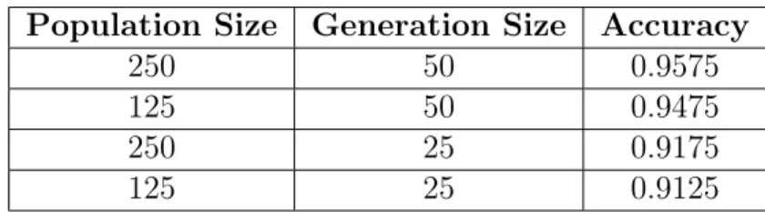
As expected, lowering either the generation or population size had a negative effect on the model’s accuracy. However, the overall loss was relatively small in comparison to the speed up in run time. By halving the population size to 125 and the generation size to 25, we achieved an accuracy of 91.25% and reduced run time 4 fold. This provides the option of prioritizing speed over model performance.

However, these two families appear to be relatively easy to separate; with scores above 90% accuracy, it is difficult to notice meaningful improvement between the subjects. In response, we selected the families of Obfuscator and OnlineGames as a

(32)

more challenging data set to separate. These families were shown in [23] to have low classification accuracy when compared against each other. Using these families as a binary classification problem, we ran the same experiments again.

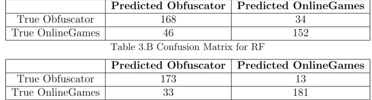
During 5 fold cross validation, NDT scored an average accuracy of 76.6%. Com-paratively, RF had a score of 88%. The results are displayed in Table 3. As expected, the models performed noticeably worse on this new challenging data set, with all models dropping around 10% accuracy or higher. Most notably, NDT is performing noticeably worse than the base models while maintaining the increased run time. However, the decrease in performance can most likely be rectified with fine tuning of hyperparameters; it still performs much better than random guessing. We also ran optimization experiments on population and generation size on this data set as well, with the results listed in Table 4.

Table 3: Confusion Matrices for Obfuscator and OnlineGames Table 3.A Confusion Matrix for NDT

Predicted Obfuscator Predicted OnlineGames

True Obfuscator 168 34

True OnlineGames 46 152

Table 3.B Confusion Matrix for RF

Table 4: Population and Generation Size Experiments for Obfuscator and OnlineGames

Population Size Generation Size Accuracy

250 50 0.8000

125 50 0.7525

250 25 0.7500

(33)

Surprisingly, the decrease in accuracy stayed relatively the same as the first optimization experiments. With a population size of 12 and a generation size of 25, we achieved an accuracy of 71.5%, which is only a 5% decrease from our cross validation results. With enough fine tuning and adjustments, acceptable accuracy may be achieved with minimal run time.

In conclusion, NDT is a viable malware classification strategy and has potential to evolve to detect malware utilizing obfuscation strategies. With these experiments completed, we elected to advance our model from decision trees to neural networks to see how more complex models interact with NEAT.

5.2 NEAT Feed Forward Neural Network

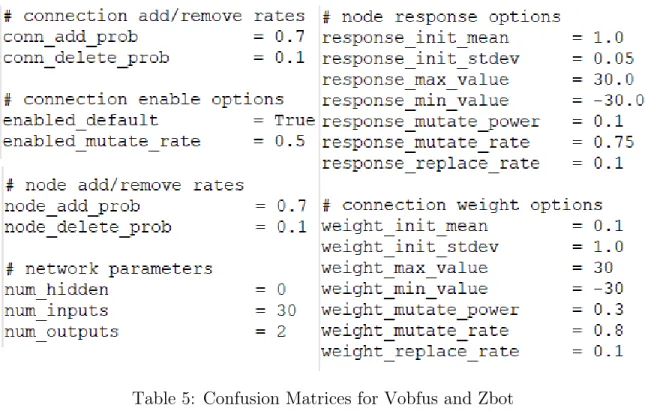
In this section, we go over the results obtained from testing the NEAT Feed Forward Neural Network (NFFNN). As discussed, this model utilizes the NEAT-Python library [31] to implement NEAT. The model we compare NFFNN against is the support vector machine (SVM) provided by the Scikit-Learn library [29]. Like the previous experiments, our data set consists of two family pairs: Vobfus and Zbot, and Obfuscator and OnlineGames. NEAT-Python runs off of a configuration file that stores the hyperparameter values used in the model. Figure 1 shows a portion of the configuration file used in our experiments. We use the same fitness function as described earlier in our NDT experiments. First, we run a standard 5-fold cross validation on both data sets for both models and compare results. Then, we perform run time optimization experiments on parameters of population and generation size. For the 5-fold cross validation testing, NFFNN ran a population of 256 for 128 generations. NFFNN managed to score an average accuracy of 96.1% for the Vobfus and Zbot pair. On the other hand, SVM scored an average accuracy of 95%. Table 5 displays the confusion matrices for each model.

(34)

Figure 1: A Selection of Hyperparameters from the NEAT Config File

Table 5: Confusion Matrices for Vobfus and Zbot Table 5.A Confusion Matrix for NFFNN

True Vobfus 193 7

True Zbot 9 191

Table 5.B Confusion Matrix for SVM

True Vobfus 200 9

True Zbot 7 184

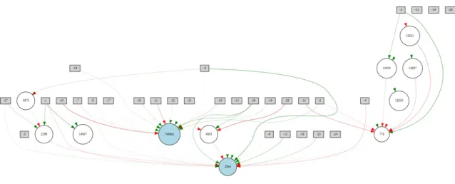
Accuracy wise, both models perform quite well in distinguishing these two malware families; there is little difference between them. This supports NEAT as a viable method to optimize classifiers for malware detection. Further optimization may produce even better results. Figure 2 shows a visualization of a top performing Neural Network generated by NEAT. The rectangles represent inputs and the two nodes

(35)

with class names are the outputs. Nodes in between were generated through random mutation and evolution, and edges are randomly disabled and enabled as well.

Figure 2: A Winning Neural Network Generated by NEAT

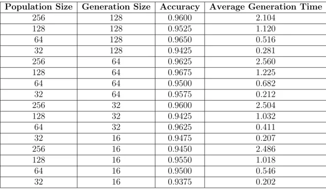
However, as with our previous experiments with NDT, run time is an issue with NFFNN. SVM was able to complete its results within a few seconds while NFFNN took nearly 5 minutes. This led us to experiment with optimizing the population and generation size parameters. The results are shown in Table 6. In addition to tracking accuracy, we measure the average time in seconds for a single generation to complete. By multiplying the time by the total number of generations, a total run time can be calculated.

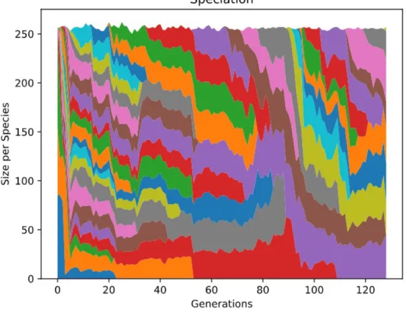
Surprisingly, the accuracy of NFFNN stays relatively stable despite having decreased both population and generation size four fold. With this, NFFNN finishes running within seconds, comparable to the speed of SVMs with similar performance. However, with such low parameter values, NFFNN is highly vulnerable to high variance in performance. For example, one of the strengths of NEAT lies in having a large enough population size to explore most possible solutions. Figure 3 displays the speciation during one run through of the NFFNN.

(36)

Population Size Generation Size Accuracy Average Generation Time

256 128 0.9600 2.104 128 128 0.9525 1.120 64 128 0.9650 0.516 32 128 0.9425 0.281 256 64 0.9625 2.560 128 64 0.9675 1.225 64 64 0.9500 0.682 32 64 0.9575 0.212 256 32 0.9600 2.504 128 32 0.9425 1.032 64 32 0.9625 0.411 32 16 0.9475 0.207 256 16 0.9450 2.486 128 16 0.9550 1.018 64 16 0.9500 0.546 32 16 0.9375 0.202

Each different color represents a different species. Some species are unable to improve and go extinct, while others dominate the field. By having so many different species, many solutions can be explored and the fittest will survive to reproduce. On the other hand, while lowering population size can improve run time, it can also prevent winning solutions from being created and tested, leading to lower performance. This can be seen in Figure 4.

As seen in this figure, with such a low population size, the number of different species drops significantly; in this case only 4 species arose, and 2 became extinct fairly quickly. This may not be an issue in situations where the data is easier to separate. In this example, it appears as if a strong solution was found immediately, which was why it dominated over the rest. However, in more difficult problems, there may not be enough genetic diversity to discover an optimal solution.

(37)

Figure 3: NEAT Species Visualization for Vobfus and Zbot: Population Size of 256

The other parameter tested in our experiments was generation size, which is another major contributor to the run time of our model. More generations allow species within the model more opportunities to mutate and evolve, fine tuning the weights towards a more optimal solution. In the case of classifying between Vobfus and Zbot, a strong solution tends to appear quite quickly. Figure 5 displays the fitness graph during one run through of the NFFNN.

In this graph there are several lines showing various fitness metrics, but the most important one is the line showing the best fitness, as this species will be selected as the winner. In this case, the best fitness starts at around 6400 which translates to about

(38)

Figure 4: NEAT Species Visualization for Vobfus and Zbot: Population Size of 32

80% accuracy based on our fitness function as mentioned in our NDT experiments. This quickly rises to over 9000 which corresponds to around 95% accuracy, matching earlier results. Once this peak is reached, little improvement to fitness is seen.

With these results, it is apparent that further generations beyond 20 serve only to increase run time with little return on investment. Finding an ideal generation size which maximizes fitness improvement is key in reaching an optimal model. However, reducing generation size by too much can result in species not having enough time to evolve and refine their strategy. Figure 6 displays the fitness graph of a model with generation size of 16.

(39)

Figure 5: Fitness Graph for Vobfus and Zbot: Generation Size of 128

Here, the best fitness line behaves similarly to that in figure 5; it rapidly reaches over 90% accuracy. However, the accuracy does not reach quite as high and may have improved with more time. Also, had the generation size been lower, the model would not have had enough time to improve.

All in all, NFFNN performs very similarly to SVMs when classifying between Vobfus and Zbot. The major difference was that NFFNN required more time to run in general, but in this case, lower population and generation size were viable solutions. However, these are still relatively easy families to distinguish. Different results may arise when dealing with more difficult families. To address this, we

(40)

Figure 6: Fitness Graph for Vobfus and Zbot: Generation Size of 16

run the experiments again using the more challenging data set of Obfuscator and OnlineGames.

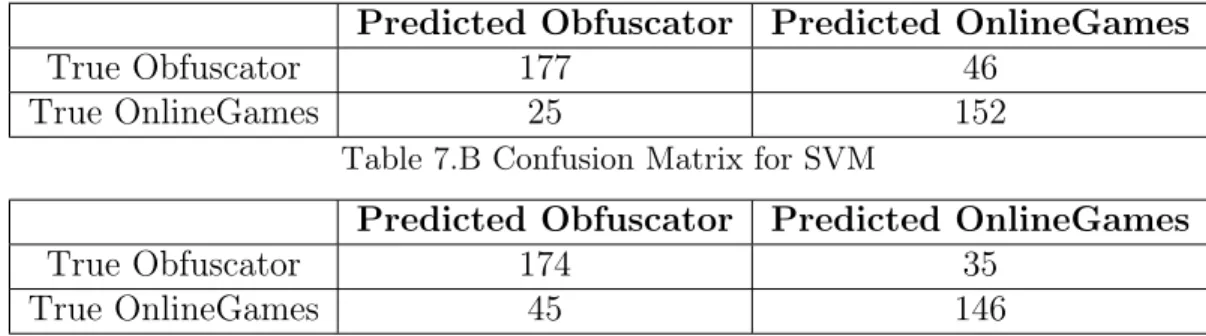
Once again, NFFNN ran a population of 256 for 128 generations for the 5-fold cross validation testing. For Obfuscator and OnlineGames, NFFNN managed to score an average accuracy of 82.25%. Comparatively, SVM scored an average accuracy of 74%. Table 7 displays the confusion matrices for each model.

Surprisingly, in this case NFFNN performed decidedly better than SVMs, by about 10%. This is the first time a NEAT model has performed so much better than a base model. This suggests that the random evolution provided by NEAT can adapt

(41)

Table 7: Confusion Matrices for Obfuscator and OnlineGames Table 7.A Confusion Matrix for NFFNN

to subtle differences in malware family better than standard SVMs. Of course, the SVM implementation we use in our experiments is by no means fully optimized for malware detection. However, this is a promising sign as our NFFNN can also benefit from fine tuning and adjustment as well. However, as discussed before NFFNN falls far behind in terms of run time. We conduct optimization experiments on population and generation size like before. The results are displayed in Table 8.

In these experiments, the trade offs between run time and model performance become much more apparent. On average, the accuracy stays around the 80% mark throughout all testing. However, as we approach lower and lower population and generation sizes, model performance becomes less consistent, occasionally dropping as low as 73%. Though this is still comparable to the performance of SVMs, it is a large drop from the peak performance of 84%.

This may be due to the issues brought up in the optimization experiments performed on Vobfus and Zbot. With a lower population size, there is not enough genetic diversity to explore solutions, and with a smaller number of generations, the species present do not have enough time to evolve. This is can be seen in Figure 7 and Figure 8.

(42)

Table 8: Population and Generation Size Experiments for Obfuscator and OnlineGames

256 128 0.8375 2.327 128 128 0.7925 1.084 64 128 0.8000 0.550 32 128 0.8425 0.253 256 64 0.8150 2.288 128 64 0.8175 1.096 64 64 0.8075 0.454 32 64 0.7900 0.254 256 32 0.8175 2.110 128 32 0.7975 1.169 64 32 0.7825 0.604 32 16 0.8050 0.298 256 16 0.8175 2.252 128 16 0.7975 1.008 64 16 0.7825 0.434 32 16 0.8050 0.203

Here, only 5 species were able to emerge with a population size of 32. Though all managed to avoid extinction, there were not enough species to fully explore optimal solutions. In the fitness graph the best fitness line made large jumps in progress, but due to a short generation time, its progress was halted before it reached a maximum.

This is due to the strength of NEAT lying in large population and generation sizes. If these are too small, there is not enough genetic diversity or time to evolve, and the model suffers. Below are a few graphs displaying the fitness growth as the model trains. Though we achieved the goal reducing run time, there were heavy concessions made in terms of accuracy.

In conclusion, NFFNN was able to reach 84% accuracy when classifying between the Obfuscator and OnlineGames families, compared to 74% scored by SVMs. This is a significant improvement, but it was offset by the large increase in run time.

(43)

Figure 7: NEAT Species Visualization for Obfuscator and OnlineGames: Population Size of 32

noticeable decreases in performance. These results suggest that NFFNN has potential to become a strong malware classifier with enough resources and fine tuning. Next, we explore using a NEAT recurrent neural network model to classify based on malware opcode sequences.

5.3 NEAT Recurrent Neural Network

In this section, we go over our final model, the NEAT Recurrent Neural Network (NRNN). This model also utilizes the NEAT-Python library [31]. We again use Scikit-Learn’s implementation of SVMs as a comparison model [29], and we utilize the same malware family pairs as previously. NRNN utilizes a similar configuration file to

(44)

Figure 8: Fitness Graph for Obfuscator and OnlineGames: Generation Size of 16

NFFNN with minor adjustments to the inputs to fit an RNN. In this experiment, the first 2000 opcodes of each malware are stored as an array and passed in as input. This is to test whether sequential information can help in detecting malware. The same fitness function is used for NRNN. First, we run a standard 5-fold cross validation on both data sets for both models and compare results. Then, we perform run time optimization experiments on parameters of population and generation size.

For the 5-fold cross validation testing, NRNN ran a population of 128 for 64 generations. NRNN managed to score an average accuracy of 94.25% for the Vobfus and Zbot pair. On the other hand, SVM scored an average accuracy of 98%. Table 9

(45)

Both models score relatively well, with SVMs scoring 4% higher than NRNN. This can be due to randomness and can be resolved through fine tuning. However, NRNN takes much more time to run compared to SVMs, as the RNN has to process 2000 inputs. This led us to try optimization experiments in order to minimize run time. The results are displayed in Table 10.

Table 9: Confusion Matrices for Vobfus and Zbot Table 9.A Confusion Matrix for NRNN

True Vobfus 194 8

True Zbot 8 190

True Vobfus 197 0

True Zbot 5 198

128 64 0.9600 39.792 64 64 0.9600 27.810 32 64 0.9650 13.844 128 32 0.9700 46.921 64 32 0.9400 26.496 32 32 0.9400 17.158 128 16 0.9700 49.561 64 16 0.7825 27.089 32 16 0.7525 11.138

In these experiments, NRNN maintains its performance relatively well, but experiences a large decrease in accuracy at the smallest generation and population

(46)

with population size 32 and generation size 16. Here we notice that the best fitness starts out quite low, and gradually increases. However, as the generation time was so short, it did not have enough time to fully optimize itself. As there were only a total of 4 species overall, this could be due to all species initializing with sub optimal weights, and struggling to improve with the genes present. Compared to Figure 11 and Figure 12, which has a population size of 128 and generation size of 32, the model managed to quickly correct its low starting fitness, most likely due to larger genetic diversity.

Figure 9: Fitness Graph for Vobfus and Zbot: Population Size of 32 and Generation Size of 16

(47)

Figure 10: NEAT Species Visualization for Vobfus and Zbot: Population Size of 32 and Generation Size of 16

All in all, these experiments show that population size may be the more important parameter to keep high. In cases of low population, the initial species can start out with poor weights that drastically slow improvement. Higher population models were able to more quickly mutate away from the sub optimal weights and reach higher accuracy. On the other hand, a longer generation size provides more opportunity for a model to correct itself. However, higher populations evolve quickly enough that lowering generation size to minimize run time may result in comparably high accuracy scores.

(48)

Figure 11: Fitness Graph for Vobfus and Zbot: Population Size of 128 and Generation Size of 32

Finally, we perform the same 5-fold cross validation experiments on the more challenging data set of Obfuscator and OnlineGames, with population size 128 and generation size 64. NRNN scored an average of 70.65% while SVMs scored an average of 82%. The confusion matrices are provided in Table 11.

In this case, NRNN performed about 10% worse than SVMs, while still maintaining a higher run time cost. We perform population size and generation size optimization experiments once more to observe its behavior. Table 12 displays the results.

(49)

Figure 12: NEAT Species Visualization for Vobfus and Zbot: Population Size of 128 and Generation Size of 32

Table 11: Confusion Matrices for Obfuscator and OnlineGames Table 11.A Confusion Matrix for NRNN

(50)

Table 12: Population and Generation Size Experiments for Obfuscator and On-lineGames

128 64 0.7475 60.714 64 64 0.6700 21.506 32 64 0.7775 11.702 128 32 0.7350 40.211 64 32 0.6225 19.435 32 32 0.6275 9.584 128 16 0.6575 35.953 64 16 0.6775 18.305 32 16 0.5725 12.052

difficult to classify, high population and generation size is necessary to take advantage of NEAT’s properties of evolution. Figure 13 and Figure 14 are the fitness and speciation graphs for population size of 32 and generation size of 16.

Once again, there are only 4 distinct species, and the best fitness starts at about 3200, which translates to about 56% accuracy. The fitness slowly improves but does not have enough time to optimize further.

All in all, NRNN performed comparatively to SVMs in the case of an easy data set, but fell behind when presented with a more challenging data set. Perhaps with more tuning, the performance can improve. However, the long run time of NRNN continues to be the main drawback when compared to traditional malware detection methods.

(51)

Figure 13: Fitness Graph for Obfuscator and OnlineGames: Population Size of 32 and Generation Size of 16

(52)

Figure 14: NEAT Species Visualization for Obfuscator and OnlineGames: Population Size of 32 and Generation Size of 16

(53)

CHAPTER 6

Conclusion and Future Work

In this paper, we have used opcode features to examine how genetic algorithms can optimize machine learning models for malware detection. Specifically, we used the NEAT algorithm to augment decision trees, feed forward neural networks, and recurrent neural networks, and compared their performance against random forest classifiers and support vector machines. We used two pairs of malware families, one easy and one challenging, for our data sets and ran multiple experiments measuring accuracy and run time.

NDT was able to perform relatively well when compared to RF; both scored above 90% accuracy on the Vobfus and Zbot data set, but performed noticeably worse on the Obfuscator and OnlineGames data set. The main difference with NDT was its increased run time compared to RF. Through optimization experiments, we determined that lowering population size and generation size massively reduced run time at the cost of accuracy.

Similarly, NFFNN performed as well as SVMs on the Vobfus and Zbot families, and managed to surpass SVMs on the more challenging Obfuscator and OnlineGames families. This suggests that NEAT powered machine learning models have the potential to outperform traditional models under the right circumstances. With further fine tuning and optimization, NFFNN could maintain a high accuracy score while minimizing run time.

NRNN maintained a high accuracy on the Vobfus and Zbot families, but struggled on the more difficult Obfuscator and OnlineGames families when compared to SVMs; NRNN scored almost 10% less accuracy than SVMs. Further experiments with lowered population size and generation size revealed the necessity of genetic diversity for neural

(54)

weights and stagnate with minimal improvement. Generation size, though it provides more opportunities for species to mutate towards stronger solutions, can usually be kept low in favor of a higher population size.

In conclusion, genetic algorithms have the potential to create effective machine learning models under the right circumstances. NEAT powered malware detection models tended to perform as well as more traditional models, and occasionally per-formed better. The concept of evolution in machine learning may be the key when dealing with malware that constantly changes to avoid detection.

6.1 Future Work

In this research we worked with a data set of malware files from known families. To our knowledge, these files were not obfuscated, nor did they change over time. If we had access to malware that had gone through stages of obfuscation at various points in time, experiments could be run to test the robustness of a NEAT malware classifier and its ability to evolve to detect newer versions of that malware family. These experiments would fully test the potential of genetic algorithms. The challenge in such a research is that metamorphic malware is quite rare in practice, and it may be difficult to procure a large enough data set for experimentation.

The primary algorithm used in or research was NEAT, but in its most basic form. Since its inception, other, more specialized versions of NEAT have been developed, such as hyper NEAT [33], which is used to evolve large-scale neural networks. Testing out these new NEAT implementations may uncover a more effective means of evolving malware classification systems.

Our research focused on malware opcodes as the primary feature for our models. There are numerous other features that can be used, such as byte data or n-grams ex-tracted from malware [6]. Utilizing different features may result in better performance

(55)

or require an entirely different implementation. The results of such experiments would undoubtedly be useful in the research of malware detection.

Finally, while this research used decision trees and neural networks as the main models being optimized by NEAT, many other valid models exist. It would be inter-esting to see how NEAT interacts with different malware classifier implementations. The challenge in such a research would be in modifying those models to be compatible with genetic algorithms. For example, NEAT encodes neural networks in a special way to more easily promote crossover between species. Finding ways of encoding other model genomes will be difficult.

(56)

LIST OF REFERENCES

[1] A. Kujawa, W. Zamora, J. Segura, T. Reed, N. Collier, J. Umawing, C. Boyd, P. Arntz, and D. Ruiz, ‘‘Malwarebytes lab: 2020 state of mal-ware report,’’ https://resources.malmal-warebytes.com/files/2020/02/2020_State- https://resources.malwarebytes.com/files/2020/02/2020_State-of-Malware-Report.pdf, 2020.

[2] V. S. Sathyanarayan, P. Kohli, and B. Bruhadeshwar, ‘‘Signature generation and detection of malware families,’’ in Information Security and Privacy, Y. Mu,

W. Susilo, and J. Seberry, Eds. Springer, 2008, pp. 336--349. [3] J. Aycock, Computer Viruses and Malware. Springer, 2006.

[4] D. Baysa, R. Low, and M. Stamp, ‘‘Structural entropy and metamorphic mal-ware,’’ Journal of Computer Virology and Hacking Techniques, vol. 9, no. 4, pp.

179--192, 2013.

[5] M. Wadkar, F. Di Troia, and M. Stamp, ‘‘Detecting malware evolution using support vector machines,’’ Expert Systems with Applications, vol. 143, 2020.

[6] S. Basole, F. Di Troia, and M. Stamp, ‘‘Multifamily malware models,’’ Journal of Computer Virology and Hacking Techniques, vol. 16, pp. 79--92, 2020. [Online].

Available: https://doi.org/10.1007/s11416-019-00345-8

[7] J. Holland, ‘‘Genetic algorithms,’’ Scientific American, vol. 267, no. 1, pp. 66--73,

1992. [Online]. Available: https://www.jstor.org/stable/10.2307/24939139 [8] Z. Bazrafshan, H. Hashemi, S. M. H. Fard, and A. Hamzeh, ‘‘A survey on

heuristic malware detection techniques,’’ in The 5th Conference on Information and Knowledge Technology, ser. IKT 2013, 2013, pp. 113--120.

[9] M. Xu, L. Wu, S. Qi, J. Xu, H. Zhang, Y. Ren, and N. Zheng, ‘‘A similarity metric method of obfuscated malware using function-call graph,’’ Journal of Computer Virology and Hacking Techniques, vol. 9, no. 1, pp. 35--47, 2013.

[Online]. Available: https://doi.org/10.1007/s11416-012-0175-y

[10] D. Gibert, C. Mateu, and J. Planes, ‘‘The rise of machine learning for detection and classification of malware: Research developments, trends and challenges,’’

Journal of Network and Computer Applications, vol. 153, p. 102526, 2020. [Online].

Available: http://www.sciencedirect.com/science/article/pii/S1084804519303868 [11] P.-N. Tan, M. Steinbach, and V. Kumar, Introduction to Data Mining. Pearson

(57)

[12] S. Shalev-Shwartz and S. Ben-David, Understanding Machine Learning: From Theory to Algorithms. Cambridge University Press, 2014.

[13] M. Stamp, Introduction to Machine Learning with Applications in Information Security. Chapman and Hall/CRC, 2017.

[14] E. A. Williams and W. A. Crossley, ‘‘Empirically-derived population size and mutation rate guidelines for a genetic algorithm with uniform crossover,’’ in Soft Computing in Engineering Design and Manufacturing, P. K. Chawdhry, R. Roy,

and R. K. Pant, Eds. Springer, London, 1998, pp. 163--172. [Online]. Available: https://doi.org/10.1007/978-1-4471-0427-8_18

[15] A. Martin, H. D. Menéndez, and D. Camacho, ‘‘Genetic boosting classification for malware detection,’’ in 2016 IEEE Congress on Evolutionary Computation (CEC), 2016, pp. 1030--1037.

[16] A. Fatima, R. Maurya, M. K. Dutta, R. Burget, and J. Masek, ‘‘Android malware detection using genetic algorithm based optimized feature selection and machine learning,’’ in 2019 42nd International Conference on Telecommunications and Signal Processing (TSP), 2019, pp. 220--223.

[17] M. Yusoff and A. Jantan, ‘‘A framework for optimizing malware classification by using genetic algorithm,’’Communications in Computer and Information Science,

vol. 180, pp. 58--72, 2011.

[18] R. L. Castro, C. Schmitt, and G. Dreo, ‘‘Aimed: Evolving malware with genetic programming to evade detection,’’ in 2019 18th IEEE International Conference On Trust, Security And Privacy In Computing And Communications/13th IEEE International Conference On Big Data Science And Engineering (TrustCom/Big-DataSE), 2019, pp. 240--247.

[19] S. Noreen, S. Murtaza, M. Z. Shafiq, and M. Farooq, ‘‘Evolvable malware,’’ in Proceedings of the 11th Annual Conference on Genetic and Evolutionary Computation, ser. GECCO ’09. New York, NY, USA:

Association for Computing Machinery, 2009, p. 1569–1576. [Online]. Available: https://doi.org/10.1145/1569901.1570111

[20] K. O. Stanley and R. Miikkulainen, ‘‘Evolving neural networks through aug-menting topologies,’’ Evolutionary Computation, vol. 10, no. 2, pp. 99--127,

2002.

[21] J. Brownlee, ‘‘A gentle introduction to the bag-of-words model,’’ https:// machinelearningmastery.com/gentle-introduction-bag-words-model/, 2019.

(58)

[22] A. Nappa, M. Z. Rafique, and J. Caballero, ‘‘The MALICIA dataset: Identifi-cation and analysis of drive-by download operations,’’ International Journal of Information Security, vol. 14, no. 1, pp. 15--33, 2015.

[23] P. Prajapati and M. Stamp, ‘‘An empirical analysis of image-based learning techniques for malware classification,’’ in Malware Analysis using Artificial Intelligence and Deep Learning. Springer, 2020.

[24] ‘‘Vobfus,’’ 2012. [Online]. Available: https://www.trendmicro.com/vinfo/us/ threat-encyclopedia/malware/vobfus

[25] ‘‘The zeus, zbot, and kneber connection.’’ [Online]. Avail-able: https://www.trendmicro.com/vinfo/us/threat-encyclopedia/web-attack/ 16/the-zeus-zbot-and-kneber-connection

[26] ‘‘Win32/obfuscator,’’ 2020. [Online]. Available: https://malwarefixes.com/ threats/win32obfuscator/

[27] ‘‘Win32/onlinegames,’’ 2017. [Online]. Available: https: //www.microsoft.com/en-us/wdsi/threats/malware-encyclopedia-description?

name=Win32/OnLineGames

[28] ‘‘pickle — python object serialization.’’ [Online]. Available: https://docs.python. org/3/library/pickle.html

[29] ‘‘scikit-learn.’’ [Online]. Available: https://scikit-learn.org/stable/ [30] ‘‘pandas.’’ [Online]. Available: https://pandas.pydata.org/

[31] ‘‘Neat-python.’’ [Online]. Available: https://neat-python.readthedocs.io/en/ latest/

[32] ‘‘Neat template.’’ [Online]. Available: https://github.com/Code-Bullet/NEAT_ Template

[33] K. O. Stanley, D. B. D’Ambrosio, and J. Gauci, ‘‘A hypercube-based encoding for evolving large-scale neural networks,’’ Artificial Life, vol. 15, no. 2, pp. 185--212,