Latent Variables and Propensity Score Matching

(1)

Warsaw 2010

No. 6/2010 (29)

Macie j Jakubowski

Latent Variables

(2)

Working Paper No. 6/2010 (29)

Latent Variables and Propensity Score Matching

Maciej Jakubowski

Faculty of Economic Sciences

University of Warsaw

[address] [e-mail]

Abstract

This paper examines how including latent variables can benefit propensity score matching. A researcher can estimate, based on theoretical presumptions, the latent variable from the observed manifest variables and can use this estimate in propensity score matching. This paper demonstrates the benefits of such an approach and compares it with a method more common in econometrics, where the manifest variables are directly used in matching. We intuit that estimating the propensity score on the manifest variables introduces a measurement error that can be limited when estimating the propensity score on the estimated latent variable. We use Monte Carlo simulations to test how various matching methods behave under distinct circumstances found in practice. Also, we apply this approach to real data. Using the estimated latent variable in the propensity score matching increases the efficiency of treatment effect estimators. The benefits are larger for small samples, for non-linear processes, and for a large number of the manifest variables available, especially if they are highly correlated with the latent variable.

Keywords:

factor analysis, latent variables, propensity score matching

JEL:

C14, C15, C16, C31, C52

Acknowledgments:

The Polish Ministry of Science and Higher Education supported this research through a grant. I thank Paweł Strawiński and Dorota Węziak-Białowolska for their comments and contributions early in this project.

Working Papers contain preliminary research results. Please consider this when citing the paper.

Please contact the authors to give comments or to obtain revised version. Any mistakes and the views expressed herein are solely those of the authors.

(3)

I. Introduction

This paper demonstrates how incorporating the latent variable modeling into the propensity score matching can limit measurement error in the propensity score and, in effect, can increase precision of the estimates of treatment effects. The idea behind this paper comes from the popularity of propensity score matching in empirical research and from economists’ distrust of latent variable modeling. In fact, in econometrics and economics the latent variable modeling is unpopular, unlike its status in sociology, psychology and psychometrics. We show that if the latent variable modeling has valid theoretical and empirical foundations, it can strongly benefit the propensity score matching.

This is not the first paper to introduce latent variable modeling into propensity score matching. The seminal work of James Heckman and others was helpful when developing the framework we present (see Abbring and Heckman, 2007, Section 2.7 for discussion and further references). However, our approach differs in one important aspect. Heckman, and others, modeled residuals from outcome equations across quasi-experimental groups assuming that there are latent traits behind them. We assume, instead, that values of the latent variable are associated with values of the manifest variables that are observable and can be used to estimate the latent variable. We present the benefits of using the estimated latent variable in the propensity score matching. The procedure we describe can notably lower the variance of treatment estimators, which we demonstrate with Monte Carlo simulations and real data examples.

The paper is organized as follows. Section II shows how the latent variables modeling can be introduced into the propensity score matching using the measurement error model of the relation between the latent trait and the manifest variables. Section III provides evidence from the Monte Carlo study on how the proposed approach increases efficiency of the matching estimators of the treatment effects. Section IV empirically applies this approach to data. Section V concludes. Appendices A and B contain additional results and a Stata software code we used to obtain results.

II. Modeling Latent Variables in Propensity Score Matching

Modeling Latent Variables

Latent variables can reflect either hypothetical constructs or existing phenomena that cannot be directly measured but are often reflected in observed variables that are proxies of measured phenomena. These observable manifestations are correlated with latent variables but also contain an independent component. Manifest variables contain a signal about the latent variable and the random component (often called the “measurement error”) that is uncorrelated with this variable.

(4)

A relation between the latent variable and the manifest variables can be presented using the one-factor model or the congeneric measurement error model (Joreskog, 1971; Skrondal and Rabe-Hesketh, 2004). We assume that the observed j-th variable is measured with error and on a scale specific to that variable. Values for a set of such manifest variables is observed for each i-th individual. This is modeled through the following equation:

ij i j j ij e Y =δ +λη + (1)

Where η is the latent variable or common factor and Yij are observed realizations of manifest variables or items. We assume that error terms eij are independent and N(0,σj). This model

can be also interpreted as a measurement error model where true scores η are reflected in each j-th variable with random error on the scale defined by δ_j and λ_j. In the factor analysis,

j

λ are called factor loadings and δ_j are called intercepts. To identify this model some restrictions are needed, for example, that λ₁=1 or that the Var(η)=1. This model assumes that there is only one latent variable behind the manifest variables; however, dealing with several latent variables is quite straightforward within this framework.

If the model we present above is true, the latent variable can be estimated from the manifest variables using factor analysis approach. Specification of a latent variable factor model has to be driven by theoretical considerations and carefully tested empirically. Usually, models assuming different numbers of common factors are estimated and compared on how they fit the data. A problem arises when such models all seem to be plausible. In this case, theoretical considerations can play an important role. In this paper, we abstract from these issues, assuming that a latent variable model properly reflects the latent structure behind the data. Moreover, we assume there is only one latent variable behind each set of manifest variables. Our approach can be easily extended to more complex situations, for example, involving more latent variables and allowing for correlations with other variables in a model. However, simple scenarios considered in this paper illustrate the main benefits of incorporating latent variables in matching. Our general findings should also hold under more complex circumstances.

We are not aware of any other study, other than the efforts of James Heckman and his colleagues described in the introduction, that attempts to model latent traits in the propensity score matching. The use of latent variables models is rare in economics or econometrics, for several reasons. First, the latent variables theory was developed outside the economics and econometrics field. Economists are not aware of modern approaches in latent variables modeling and are suspicious about assuming the existence of latent traits when modeling economic phenomena. Second, typical datasets used by economists do not contain information that can be used to estimate latent variables. In labor market studies, where propensity score matching is relatively widely used, questions about attitudes or opinions are rarely available. In administrative data such information is never present, while in labor force surveys these types of questions are infrequent and are usually limited to one or two direct questions instead of a set of questions that can be used to estimate the latent attitude.

(5)

The usefulness of latent variable modeling in economic research can be reconsidered when taking into account modern developments in statistics. Recent work demonstrates that current approaches are much more reliable, are theory driven and are more adverse to ad hoc interpretations (see Skrondal and Rabe-Hesketh, 2004, for an extensive discussion and unifying framework). Moreover, in many circumstances, such as evaluating labor market training or school programmes, latent traits like attitudes play an important role in the choices of participants and non-participants. In educational studies, numerous works demonstrate how important for student performance are attitudes or latent family characteristics (OECD, 2009; Jakubowski and Pokropek, 2009). In labor market studies, it was shown that job satisfaction, even if measured through a single simple question, significantly changes quasi-experimental estimates (White and Killeen, 2002).

Usually, instead of modeling latent traits directly, economists use survey responses that reflect these traits. In studies of anti-poverty programmes direct responses about household possessions are typically used (see Jalan and Ravallion, 2003), although they could be modeled as latent traits reflecting household wealth and socio-economic position (we use a similar example in this paper). In a well-known paper by Agodini and Dynarski (2004) on propensity score matching, student responses to questions about time use and attitudes towards learning were added to the list of matching covariates instead of being used to model the latent characteristics behind them. While similar examples are rare in economic literature, this is not because information on latent traits is useless or impossible to obtain. It seems that economists simply do not make attempts to use such information. We hope that this paper will contribute to changing this situation.

We propose an approach where the latent variable is estimated from the manifest variables and directly used in the propensity score matching. A similar approach is widely used in educational research or psychology where latent constructs are estimated and then used in regression or other statistical models. Our paper presents benefits of using the estimated latent variable instead of a set of manifest variables in the propensity score matching. Simulation results and empirical examples demonstrate that modeling latent variable increases precision of propensity score matching estimates of treatment effects.

Propensity Score Matching with Latent Variables

Consider a situation where we want to compare outcomes between two groups where the latent variable is unbalanced. One of these quasi-experimental groups is affected by a treatment, while the other remains unaffected and serves as a baseline reference group. We call subjects in the first group the “treated” and subjects in the latter group the “controls.” We assume that the latent variable affects outcomes in both groups, and that the unbalance in the latent variable creates bias when comparing group outcomes.

For observational studies, a matching approach was proposed to balance covariates among groups of treated and controls (Rubin, 1973). Propensity score matching is currently the most popular version of this approach and is based on balancing covariates through

(6)

matching conducted on a propensity score (Rosenbaum and Rubin, 1983). Propensity score is usually estimated by logit or probit and reflects the probability of being selected to the group of treated. Matching based on the propensity score instead of matching on all covariates solves the so-called curse of dimensionality that makes normal matching inadvisable or even impossible in smaller samples. After balancing covariates by using matching, simple outcome comparisons provide unbiased estimates of treatment effects, assuming that all differences between the two groups are observed and taken into account when estimating the propensity score (see Heckman et al., 1998, for detailed assumptions).

Consider that not only the unbalance of the observed covariates, but also the unbalance of the latent variable, poses a potential barrier to estimate treatment effects. In this case, a researcher would like to include the latent variable in matching, however, that is not observed. Instead, matching has to be conducted on the observed variables, including the manifest variables that are only proxies of the latent trait. By assumption, the manifest variables reflect the latent variable with a random error. Estimating the propensity score on the manifest variables introduces additional noise into matching. Intuitively, the greater the error, the more often are subjects mismatched, which affects the quality of matching estimators. The smaller the error is or the stronger a signal from the latent variable reflected in the manifest variables is, the more negligible is the fact that matching is not conducted directly on the latent variable.

This paper discusses how estimating the latent variable, and conducting matching on this estimate rather than on a set of manifest variables, can increase the quality of matching in some situations, especially in smaller samples or with a relatively weak signal about the latent variable available in the manifest variables. Compared to the observable proxies, the estimated latent variable should reflect the latent variable with more precision if the latent variable model is correct. This will benefit matching, as less error is introduced.

More formally, consider first a hypothetical situation where the latent variable is directly observed and can be used for matching. In this case, a propensity score is given by:

ε

δη

α

η

= +Xβ+ + X, ) ₀ ( P (2)

Where η is the latent variable that has to be balanced together with other covariates contained in the vector X. After successful matching, which balances the latent variable and other covariates among quasi-experimental groups, the average treatment effects can be estimated through simple comparisons of outcomes in a group of treated and matched controls.

ATT = Y[P(X,η),D=1] - Y[(P(X,η),D=0] (3)

Where Y is an outcome and D=0,1 denotes the treatment status (D=1 for treated).

In practice, the latent variable is never observed. One way to overcome that is to estimate the propensity score using information on the latent variable reflected in a set of manifest variables: ε α + + + = Xβ Mδ M X ₀ *₍ _, ₎ P (4)

(7)

This introduces a measurement error to the propensity score, because manifest variables are imperfect reflections of the latent variable. If the manifest variables are generated from the latent variable by adding a random noise, then the measurement error in the propensity score is also random. The average treatment effects can be calculated using equation (3) by substituting P(X,η) with *( , )

M X

P .

We propose a different approach that is not discussed in the matching literature. In this approach the latent variable is estimated from the manifest variables. We assume that the latent structure and the model to estimate it follow the one described by the set of equations (1), that one latent factor is reflected in the observed manifest variables. In this case, the latent variable can be estimated by the factor analysis model, and this latent-variable estimate can be used to obtain the propensity score:

ε η α ηˆ)= + + ˆ+ , ( ₀ * δ P X βx (5)

where ηˆ is the estimated latent variable. The average treatment effects can be calculated using equation (3) by substituting P*(X,

η

ˆ) for P(X,η).

We describe, above, three propensity scores that can be used for balancing the latent variable and covariates through the propensity score matching: the hypothetical propensity score P(X,η) estimated on the unobservable latent variable, the typically used propensity score P*(X,M) that is estimated from the observed manifest variables, and finally the propensity score P*(X,

η

ˆ) obtained by first estimating the latent variable from the manifest variables and then by using this estimate to obtain the propensity score. This paper addresses the question of how using a quality of matching differs when using the three different propensity scores. We address this through a simulation study where matching is conducted under various circumstances commonly found in practice of empirical research. In simulation, we can compare the results obtained with the hypothetical propensity score estimated using the unobserved latent variable with results obtained with error-prone propensity scores used in practice. In Section III, we also give a real-life example of applying the strategy suggested by simulation results to data from educational study.

III. Simulation Study

We conducted our simulation study in two parts. In the first part, we studied a simple linear data generating process with random treatment assignment and balanced covariates. This gave us an overall idea of how modeling latent variables in the propensity score matching can affect standard errors of the average treatment effects. In the second part, we studied a more complicated data generating process, with non-random selection and highly non-linear relations between the latent variable and an outcome. This case provides more insights into how modeling latent variables affects bias and the precision of matching estimators under differing circumstances. In all simulations, 10,000 random draws were studied.

(8)

Simulation A: No Selection, Normally Distributed Latent Variable with Linear Relation to Outcome

Assume that the outcome generating process can be described by this simple equation:

ε η+ + + − = T y 10 5 3 (6)

The outcome depends linearly on the normally distributed latent variable η (with mean 0 and standard deviation 1), and the treatment effect is equal to 3 for all treated subjects, who are indicated by T=1. Selection to quasi-experimental groups is purely random, with a third of the subjects assigned to the treated group. Although values of the latent variable are observed in our simulation, we assume that a researcher observes only manifest variables that are generated by a set of equations:

j

j k

M =η+ ε , (7)

where Mjdenotes the j-th manifest variable constructed from the latent variable η by adding a random noise εj specific to each manifest variable. Correlation between the latent variable and the manifest variables depends on a signal-to-noise ratio captured in a parameter k that is studied in the simulation. For example, with k=2 the signal-to-noise ratio equals 1:2, which means that correlation between the latent variable and a manifest variable is close to 0.45. We studied also the results for values of k equal to 1 and 5 where correlation between the latent variable and a manifest variable is close to 0.7 and 0.2 respectively. This gives a typical range found in empirical research. In practice, when correlation of manifest variables (commonly called “items”) is weaker than 0.3-0.4, that is usually taken as a sign that this variable has no relation to the latent construct. In such a case, the variable is usually dropped and other manifest variables are used.

We also varied the number of manifest variables from which a researcher can estimate the latent variable. Usually, the higher the number of manifest variables is, the better an estimate of the latent variable is. We simulated data with 5, 10, 20 and 50 manifest variables, the range that covers typical situations. The quality of the estimated latent variable depends also on the sample size. We studied sample sizes with 100, 500, 1,000 and 5,000 observations that cover a range typically found in practice.

For each simulated sample, the propensity score matching was conducted three times. First, matching was conducted on the latent variable that is normally unobserved. That gives a proper baseline for further comparisons. Second, matching was conducted on the set of manifest variables. Finally, matching was conducted on the estimated latent variable using information reflected in the manifest variables. We estimated the latent variable through a basic one-dimensional factor model using a standard procedure in Stata software (see Stata documentation on the -factor- command; see Appendix B with Stata code for details). This model reflects the process in which manifest variables were generated. This assumes that the model used for the latent variable estimation was correctly specified. Obviously, that is not always the case in empirical research. But, we do not study how mistakes in estimation of the

(9)

latent variable can affect the quality of matching, we simply assume this step was conducted properly.

Finally, each propensity score was employed in two types of propensity score matching: 1-to-1 nearest neighbor matching, and local linear regression (llr) matching. Those were compared with results from a simple linear regression model. The nearest neighbor 1-to-1 matching assigns, for each treated subject, one control subject that has the closest value of the propensity score. The llr matching estimates, for each treated subject, a predicted outcome among those controls that are close in values of the propensity score, weighting observations by proximity in the propensity score (see Smith and Todd, 2005, for a description of different matching methods).

We hypothesize that distinct matching methods will be affected differently by the measurement error present in the propensity score. We expect that distinct matching estimators will behave differently when matching is conducted on the latent variable, on the set of observed manifest variables, or on the estimated latent variable. The intuition behind this presumption is that, in the 1-to-1 method, the quality of matching depends more on the quality of the propensity score because only one subject is identified for each treated. Mistakenly assigning a wrong subject from a pool of controls can be costly in this method. The llr method uses all information available for subjects with similar propensity score values, which can limit the impact of measurement error according to our expectations.

Results for the simulation A study are presented in Tables 1 and 2. These demonstrate how using the manifest variables instead of the latent variable lowers the quality of matching estimates and how matching based on the estimated latent variable can help. Generally, results presented in Table 1 demonstrate that all methods are able to properly recover the value of treatment effect. For only the sample of 100 observations, mean estimates are slightly lower than the true value of 3, but only when matching is not conducted on the latent variable.

Table 1. Mean estimate of the average treatment effect in simulation A

Sample size

Regression Propensity Score Matching

nearest neighbor (1-to-1) local linear regression (llr)

latent manifest estimated _latent latent manifest estimated _latent latent manifest estimated _latent

100 2.998 2.999 2.997 3.000 2.997 2.997 3.000 2.996 2.997 500 3.000 3.000 3.000 3.000 2.999 3.000 3.000 3.000 3.000 1000 3.000 3.000 3.000 3.000 3.001 3.000 3.000 3.000 3.000 5000 3.000 3.000 3.000 3.000 3.000 3.000 3.000 3.000 3.000

Table 2 shows results on a variance of the analyzed estimators. Mostly, regression outperforms matching for sample sizes smaller than 5,000, which is not surprising as we simulated data generated by a simple linear process. From a practical point of view, more intriguing are comparisons between two matching methods with a crucial distinction between matching on the set of manifest variables and matching on the estimated latent variable.

(10)

Matching on the estimated latent variable clearly outperforms matching on the set of manifest variables. However, the difference diminishes according to sample size and is smaller for the llr matching than for the 1-to-1 matching. The 1-to-1 method provides estimates with higher variance than does the llr method. Note also that for a sample size of 1,000 the difference between matching on the estimated latent variable and the set of manifest variables in case of the llr matching is slight, while there is still substantial difference for the 1-to-1 matching. For a sample size of 5,000, the llr matching provides estimates of similar quality to those obtained through a simple linear regression, with no difference between matching on the estimated latent variable or on the set of manifest variables. This difference is still substantial for the 1-to-1 matching.

Table 2. Standard deviation of the average treatment effect estimates in simulation A

Sample size

nearest neighbor (1-to-1) local linear regression (llr)

latent manifest estimated

latent latent manifest

estimated

latent latent manifest

estimated latent 100 0.215 0.628 0.596 0.305 2.611 0.803 0.304 2.608 0.798 500 0.096 0.255 0.255 0.131 0.516 0.344 0.101 0.308 0.264 1000 0.067 0.177 0.177 0.091 0.355 0.240 0.069 0.195 0.181 5000 0.030 0.079 0.079 0.041 0.157 0.107 0.030 0.081 0.079

Table 3 presents more results on the variance of estimators for the two propensity score matching methods, separately for different numbers of manifest variables and for different signal-to-noise ratios. Generally, the results confirm that for the simple linear data, generating process matching on the estimated latent variable noticeably reduces the variance of estimators in comparison to matching on the set of manifest variables. The results confirm also that in this baseline case the llr matching clearly outperforms the 1-to-1 matching for samples bigger than 100. For example, with the 1-to-1 method in the case of 10 manifest variables, a sample size of 500 and a signal-to-noise ratio 1:1, the standard deviation of the average treatment effects when matching on the manifest variables is equal to 0.47; it goes down to 0.24 when matching on the estimated latent variable. Similar numbers for the llr method are 0.23 and 0.18, which suggests that this method provides more efficient estimators.

Detailed results in Table 3 show how the number of manifest variables affects variance of the estimators. Looking again at results for a sample size of 500 and a signal-to-noise ratio of 1:1, we see that in matching on the estimated latent variable, variance of the estimators goes down with the number of manifest variables, but it remains the same when matching directly on the manifest variables. This is less true for bigger sample sizes where matching on the estimated latent variable still outperforms matching on the manifest variables, but both methods benefit from the higher number of manifest variables available.

Results for the smallest sample of 100 observations reveal intriguing patterns. In this case, introducing more manifest variables noticeably increases the variance for matching

(11)

estimators based on the full set of manifest variables; while for matching on the estimated latent variable, the variance decreases with the number of manifest variables. It seems that in smaller samples, estimation of the propensity score is too demanding when too many manifest variables are considered; in this case increasing the number of these variables does not help. These results clearly show that, in small samples, researchers should never match directly on the manifest variables if there are too many of them in relation to a sample size. Matching on the estimated latent variable is clearly preferred in this case.

The results for moderately large samples and different signal-to-noise ratios demonstrate how important it is to base matching on a larger set of manifest variables, especially when they are highly correlated with the unobservable latent variable. For matching on the estimated latent variable and a signal-to-noise ratio of 1:1, even with a sample size of 1,000 and 20 or 50 manifest variables, both matching methods have variance quite close to the one obtained with matching directly on the latent variable. That is not the case for higher signal-to-noise ratios, for example, with a ratio of 1:5 even with a sample of 5,000 observations and 50 manifest variables, variances of matching estimators are two or more times higher than the variances for estimators based on matching on the latent variable.

Higher noise in the manifest variables reduces the relative benefits of matching on the estimated latent variable instead of matching on the set of manifest variables, especially for situations with a higher number of observed manifest variables. While the first method still outperforms the latter, it is clear that the benefits of using the estimated latent variable in matching are much higher when the manifest variables strongly correlate with the latent variable, especially if the number of these variables observed to the researcher is relatively high. For example, with 5 manifest variables, a signal-to-noise ratio equal to 1:1 and a sample size of 500, the standard deviation of the 1-to-1 matching estimators is equal to 0.47 when matching on the manifest variables and 0.29 when matching on the estimated latent variable. With 50 manifest variables available, the difference is much bigger with respective standard deviations equal to 0.50 and 0.16. However, with 5 noisy manifest variables with a signal-to-noise ratio of 1:5, the same difference is much smaller with respective numbers of 0.54 and 0.45, and it grows only moderately if 50 manifest variables are available, giving a standard deviations equal to 0.54 and 0.30, respectively.

(12)

Table 3. Standard deviation of the average treatment effect estimates

Sample

size Matching on the:

Nearest Neighbor Matching (1-to-1) Local Linear Regression Matching (llr) number of manifest variables number of manifest variables

5 10 20 50 5 10 20 50 Signal-to-noise ratio 1:1 100 latent 0.31 0.31 0.30 0.30 0.31 0.30 0.30 0.30 manifest 1.06 1.13 1.28 4.71 1.05 1.12 1.27 4.71 estimated latent 0.67 0.53 0.44 0.37 0.66 0.53 0.43 0.37 500 latent 0.13 0.13 0.13 0.13 0.10 0.10 0.10 0.10 manifest 0.47 0.47 0.47 0.50 0.25 0.23 0.22 0.26 estimated latent 0.29 0.24 0.19 0.16 0.22 0.18 0.15 0.12 1000 latent 0.09 0.09 0.09 0.09 0.07 0.07 0.07 0.07 manifest 0.32 0.33 0.32 0.34 0.16 0.14 0.13 0.13 estimated latent 0.21 0.16 0.13 0.11 0.15 0.12 0.10 0.08 5000 latent 0.04 0.04 0.04 0.04 0.03 0.03 0.03 0.03 manifest 0.15 0.14 0.14 0.14 0.07 0.06 0.05 0.04 estimated latent 0.09 0.07 0.06 0.05 0.07 0.05 0.04 0.04 Signal-to-noise ratio 1:2 100 latent 0.31 0.31 0.30 0.30 0.31 0.30 0.30 0.30 manifest 1.23 1.23 1.34 4.80 1.22 1.22 1.33 4.80 estimated latent 1.00 0.84 0.68 0.50 0.99 0.83 0.67 0.50 500 latent 0.13 0.13 0.13 0.13 0.10 0.10 0.10 0.10 manifest 0.53 0.51 0.50 0.52 0.36 0.31 0.28 0.29 estimated latent 0.45 0.37 0.29 0.22 0.35 0.28 0.23 0.17 1000 latent 0.09 0.09 0.09 0.09 0.07 0.07 0.07 0.07 manifest 0.37 0.36 0.35 0.34 0.24 0.20 0.17 0.16 estimated latent 0.32 0.26 0.21 0.15 0.24 0.19 0.15 0.12 5000 latent 0.04 0.04 0.04 0.04 0.03 0.03 0.03 0.03 manifest 0.17 0.16 0.15 0.15 0.11 0.09 0.07 0.06 estimated latent 0.14 0.11 0.09 0.07 0.10 0.08 0.07 0.05 Signal-to-noise ratio 1:5 100 latent 0.31 0.31 0.30 0.30 0.31 0.30 0.30 0.30 manifest 1.23 1.27 1.40 4.74 1.22 1.26 1.40 4.74 estimated latent 1.03 1.00 0.91 0.72 1.03 0.99 0.91 0.72 500 latent 0.13 0.13 0.13 0.13 0.10 0.10 0.10 0.10 manifest 0.54 0.53 0.53 0.54 0.36 0.34 0.32 0.32 estimated latent 0.45 0.42 0.37 0.30 0.35 0.32 0.29 0.23 1000 latent 0.09 0.09 0.09 0.09 0.07 0.07 0.07 0.07 manifest 0.37 0.37 0.37 0.36 0.24 0.23 0.21 0.19 estimated latent 0.32 0.29 0.26 0.21 0.24 0.22 0.19 0.16 5000 latent 0.04 0.04 0.04 0.04 0.03 0.03 0.03 0.03 manifest 0.17 0.17 0.16 0.15 0.10 0.10 0.09 0.07 estimated latent 0.14 0.13 0.12 0.09 0.10 0.10 0.09 0.07

(13)

Simulation B: Selection, Skewed Distribution of the Latent Variable and Non-Linear Relation with an Outcome

Simulation A assumes that the data generating process was linear in the randomly distributed latent variable. Not surprisingly, linear regression behaves better than matching in such circumstances. However, matching can outperform regression if the data generating process is non-linear and when matching covariates are highly unbalanced across quasi-experimental groups. Simulation B models similar conditions, namely, that the latent variable is unbalanced across the two groups and its relation with an outcome is non-linear. Our simulation strategy follows the one proposed by Frölich (2004). However, we model distributions of the latent variable while Frölich studied various distributions of the propensity score.

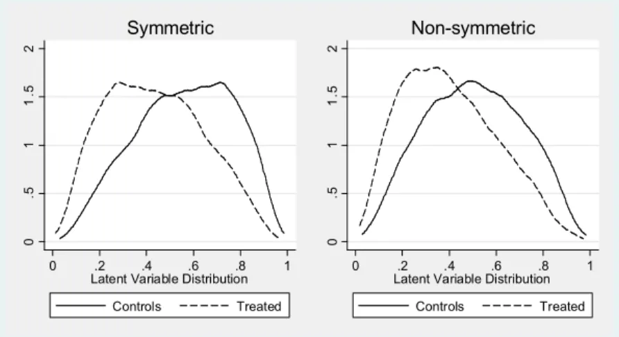
We assume that the latent variable has a Johnson SB distribution, which is unbalanced across randomly assigned treatment and control groups. We study two cases. In the first, distribution of the latent variable in one of the groups mirrors distribution in the other one. In the second, the latent variable is symmetrically distributed while distribution for the treated subjects is highly skewed. Figure 1 gives an example of the latent variable distribution in both scenarios.

The advantage of using the Johnson SB distribution for our application is that it has big probability mass in the tails so that, for each value of the latent variable of the treated, there are always possible matches among controls. In other words, the common support requirement is always fulfilled. However, with an outcome non-linearly dependent on the latent variable, comparisons for subjects at the tails of distribution can be demanding. Details on how we obtained these distributions are available in the Stata code in Appendix B.

Figure 1. Latent variable distribution for the simulation with symmetric and non-symmetric designs 0 .5 1 1 .5 2 0 .2 .4 .6 .8 1 Latent Variable Distribution

Controls Treated Symmetric 0 .5 1 1 .5 2 0 .2 .4 .6 .8 1 Latent Variable Distribution

Controls Treated Non-symmetric

(14)

As in the previous simulations, we construct the manifest variables by adding random noise to the latent variable with different signal-to-noise ratios. Random noise variables were scaled to have the same standard deviation as the latent variable with Johnson SB distribution. This allows signal-to-noise ratio comparisons with the results from Simulation A.

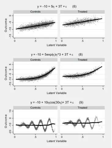
Finally, we studied three data generating processes: the one studied in Simulation A and given by equation (6) and two additional processes that are given by the following equations: ε η η + + + − = T y 10 5exp( ) ^3 3 (8) ε η η + + + − = T y 10 10 cos(30 ) 3 (9)

The equations differ in the form of relation between an outcome and the latent variable. While equation (6) mirrors the linear process studied in Simulation A, equation (8) models a curvilinear relation of the latent variable and an outcome. Equation (9) gives a highly non-linear process. Figure 2 provides graphical examples of the relation between the latent variable and an outcome across two quasi-experimental groups and for three data-generating processes.

Figure 2. Three outcome equations from Simulation B

-1 5 -1 0 -5 0 0 .5 1 0 .5 1 Controls Treated O u tc o m e Latent Variable y = -10 + 5η + 3T + ε (6) -1 5 -1 0 -5 0 5 0 .5 1 0 .5 1 Controls Treated O u tc o m e Latent Variable y = -10 + 5exp(η)η^3 + 3T + ε (8) -2 0 -1 0 0 1 0 0 .5 1 0 .5 1 Controls Treated O u tc o m e Latent Variable y = -10 + 10ηcos(30η)+ 3T + ε (9)

(15)

As previously, we studied scenarios reflecting circumstances typically found in empirical research. As we compared the results for outcome equations and symmetric or non-symmetric distributions, we limited the number of simulation parameters. We considered only two values of signal-to-noise ratio (for k equal to 1 and 2, not for 5), three numbers of manifest variables (5, 10 and 50, not for 20), and two sample sizes (only 500 and 5,000). Again, for each simulated sample, we conducted the propensity score matching three times: once with the normally unobserved latent variable, once with a set of observed manifest variables, and once with the latent variable estimated using the simple one-factor model. As previously, we studied two types of matching estimators, namely, the 1-to-1 nearest neighbor matching and the local linear regression matching. We compared those with the results from a simple linear regression.

Tables 4 and 5 present detailed results for the two matching methods: for the design with symmetrically distributed latent variable; and for different sample sizes, numbers of manifest variables and signal-to-noise ratios. In Appendix A, we present the overall mean results, which make a distinction for sample size only (Tables A3 and A4). We also present the results for the non-symmetric design in Appendix A (Tables A5 and A6). Generally, they resemble the results for the symmetric case.

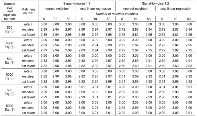
Table 4. Mean estimates of average treatment effect for the symmetric design

Sample size and equation number Matching on the: Signal-to-noise 1:1 Signal-to-noise 1:2

nearest neighbor local linear regression nearest neighbor local linear regression

Number of manifest variables

5 10 50 5 10 50 5 10 50 5 10 50 500 Eq. (6) latent 3.00 3.00 3.00 3.00 3.00 3.00 3.00 3.00 3.00 3.00 3.00 3.00 manifest 2.89 2.94 2.97 2.89 2.94 2.97 2.72 2.82 2.94 2.72 2.82 2.94 est.latent 2.89 2.94 2.98 2.89 2.94 2.98 2.72 2.82 2.95 2.72 2.82 2.95 5000 Eq. (6) latent 3.00 3.00 3.00 3.00 3.00 3.00 3.00 3.00 3.00 3.00 3.00 3.00 manifest 2.89 2.94 2.98 2.89 2.94 2.98 2.72 2.82 2.95 2.72 2.82 2.95 est.latent 2.89 2.94 2.99 2.89 2.94 2.99 2.72 2.82 2.95 2.72 2.82 2.95 500 Eq. (8) latent 3.00 3.00 3.00 3.00 3.00 3.00 3.00 3.00 3.00 3.00 3.00 3.00 manifest 2.82 2.90 2.97 2.82 2.90 2.97 2.50 2.69 2.91 2.50 2.69 2.91 est.latent 2.82 2.90 2.98 2.82 2.90 2.97 2.50 2.69 2.91 2.50 2.69 2.92 5000 Eq. (8) latent 3.00 3.00 3.00 3.00 3.00 3.00 3.00 3.00 3.00 3.00 3.00 3.00 manifest 2.82 2.90 2.98 2.82 2.90 2.97 2.51 2.69 2.92 2.51 2.69 2.92 est.latent 2.82 2.90 2.98 2.82 2.90 2.98 2.51 2.69 2.92 2.51 2.69 2.92 500 Eq. (9) latent 3.00 3.00 3.00 3.01 3.01 3.01 3.00 3.00 3.00 3.01 3.01 3.01 manifest 2.99 3.00 3.00 2.99 3.00 3.00 2.99 3.00 3.00 2.99 2.99 3.00 est.latent 2.99 3.00 3.00 2.99 3.01 3.01 2.99 3.00 2.99 2.98 3.00 3.00 5000 Eq. (9) latent 3.00 3.00 3.00 3.00 3.00 3.00 3.00 3.00 3.00 3.00 3.00 3.00 manifest 3.00 3.00 3.00 3.00 3.01 3.01 2.99 2.99 3.00 2.99 3.00 3.00 est.latent 3.00 3.00 3.00 3.00 3.01 3.01 2.99 2.99 3.00 2.99 3.00 3.01

(16)

The results in Table 4 clearly demonstrate that bias in the average treatment effect estimates is similar for matching on the set of manifest variables and matching on the estimated latent variable. In both cases, the results are slightly biased. They approach the true value for the higher number of the manifest variables and for a stronger signal from the latent variable. There is also no difference between the 1-to-1 method and the llr method in terms of estimates bias. Both methods provide very similar results that replicate the true value when the unobservable latent variable is used in matching or in the most favorable circumstances (large sample, high number of manifest variables and strong signal from the latent variable).

The bias is noticeably high when only a low number of noisy manifest variables is available. Sample size plays a less important role here. The bias also visibly increases in non-linear designs. With only 5 manifest variables and signal-to-noise ratio of 1:2, the bias is relatively high for an outcome simulated by equation (8). In many cases, simulated circumstances are not far from those encountered in practice. The results suggest that having a large pool of informative manifest variables is needed to limit bias in treatment estimates.

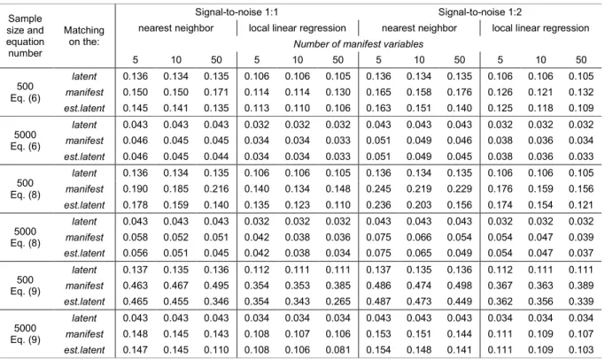
We now turn to discussing the variance of these estimators, for which standard deviations across 10,000 replications are presented in Table 5. Generally, the variance of the estimators decreases with the sample size and is smaller when the manifest variables contain a stronger signal about the latent variable. Compared to the linear outcome relation in equation (6), the variance increases for the exponential relation under equation (8) and is noticeably higher in a demanding, highly non-linear setting under equation (9). Variance is always smaller for the llr method than for the 1-to-1 method.

Table 5. Standard deviation of the average treatment effect estimates in the symmetric design

Sample size and equation number Matching on the: Signal-to-noise 1:1 Signal-to-noise 1:2

nearest neighbor local linear regression nearest neighbor local linear regression

Number of manifest variables

5 10 50 5 10 50 5 10 50 5 10 50 500 Eq. (6) latent 0.136 0.134 0.135 0.106 0.106 0.105 0.136 0.134 0.135 0.106 0.106 0.105 manifest 0.150 0.150 0.171 0.114 0.114 0.130 0.165 0.158 0.176 0.126 0.121 0.132 est.latent 0.145 0.141 0.135 0.113 0.110 0.106 0.163 0.151 0.140 0.125 0.118 0.109 5000 Eq. (6) latent 0.043 0.043 0.043 0.032 0.032 0.032 0.043 0.043 0.043 0.032 0.032 0.032 manifest 0.046 0.045 0.045 0.034 0.034 0.033 0.051 0.049 0.046 0.038 0.036 0.034 est.latent 0.046 0.045 0.044 0.034 0.034 0.033 0.051 0.049 0.045 0.038 0.036 0.033 500 Eq. (8) latent 0.136 0.134 0.135 0.106 0.106 0.105 0.136 0.134 0.135 0.106 0.106 0.105 manifest 0.190 0.185 0.216 0.140 0.134 0.148 0.245 0.219 0.229 0.176 0.159 0.156 est.latent 0.178 0.159 0.140 0.135 0.123 0.110 0.236 0.203 0.156 0.174 0.154 0.121 5000 Eq. (8) latent 0.043 0.043 0.043 0.032 0.032 0.032 0.043 0.043 0.043 0.032 0.032 0.032 manifest 0.058 0.052 0.051 0.042 0.038 0.036 0.075 0.066 0.054 0.054 0.047 0.039 est.latent 0.056 0.051 0.045 0.042 0.038 0.034 0.075 0.065 0.049 0.054 0.047 0.037 500 Eq. (9) latent 0.137 0.135 0.136 0.112 0.111 0.111 0.137 0.135 0.136 0.112 0.111 0.111 manifest 0.463 0.467 0.495 0.354 0.353 0.385 0.486 0.474 0.498 0.367 0.363 0.389 est.latent 0.465 0.455 0.346 0.354 0.343 0.265 0.487 0.473 0.449 0.362 0.356 0.339 5000 Eq. (9) latent 0.043 0.043 0.043 0.034 0.034 0.034 0.043 0.043 0.043 0.034 0.034 0.034 manifest 0.148 0.145 0.143 0.108 0.107 0.106 0.153 0.151 0.144 0.111 0.109 0.107 est.latent 0.147 0.145 0.110 0.108 0.106 0.081 0.154 0.148 0.141 0.111 0.109 0.103

(17)

The most instructive results are for comparisons between matching on the set of manifest variables and matching on the estimated latent variable. Generally, the latter method outperforms the first. The benefits of matching on the estimated latent variable are greater for smaller sample sizes, with a high number of manifest variables observed, for non-linear data generating processes, and for the 1-to-1 matching. The difference is relatively small for samples of 5,000, but clearly visible with only 500 observations available. Under this simulation design, even with a moderate sample size of 500 the variance of estimators increases with the number of manifest variables when matching is conducted directly on them and when the manifest variables contain a relatively strong signal. This is more evident for the 1-to-1 matching and less true with noisy manifest variables. This result seems to be intuitive, with a trade-off between using more information and estimating the propensity score on a relatively small sample size and with a relatively large set of covariates. We suggest that, for moderate sample sizes, researchers should never match directly on the manifest variables. In smaller samples with a high number of informative manifest variables, estimating the latent variable and matching based on this estimate is preferable.

In the linear setting with larger samples, the benefits of having more manifest variables and matching on the estimated latent variable instead of matching directly on the manifest variables are not evident. However, the benefits of using the estimated latent variable are quite clear for non-linear processes. For non-linear cases, the variance decreases with the number of manifest variables, especially when matching on the estimated latent variable. Interestingly, with a strong signal contained in the manifest variables when the outcome is generated non-linearly, as with equation (9), even in large samples, having more manifest variables of high quality does not help. The variance stays at the same relatively high level even with 50 manifest variables and 5,000 observations. Under the same circumstances, the variance diminishes when matching is conducted on the estimated latent variable. For a moderate sample size of 500, variance can even increase when matching on a higher number of manifest variables with the outcome generated through a highly non-linear process. However, when using information from manifest variables to estimate the latent variable in the first step and then to use it in matching, having more manifest variables helps to reduce variance, especially if the manifest variables contain a strong signal about the latent trait and a low level of random noise.

IV. Empirical Application to Educational Research

Simulation results suggest that estimating the latent variable from the manifest variables instead of using these variables directly in matching can increase the precision of the treatment estimates, especially with moderate sample sizes and several manifest variables available in a dataset. The suggested procedure has three steps. In the first step, a researcher has to estimate the latent variable from the observed manifest variables. This step is crucial and has to be based on theoretically and empirically sound theory that relates observed manifest variables to the latent variable. In the next steps, the usual propensity score matching approach is applied. The propensity score is estimated on a set of matching

(18)

covariates that includes the estimated latent variable. Matching is conducted on this propensity score, and the average treatment effect is calculated.

In this section, we apply this approach to educational research, using a subset of data collected in the PISA survey. The PISA study is conducted by the OECD every three years and measures the achievement of 15-year-olds across all OECD countries and other countries that join the project (see OECD, 2007, 2009, for a detailed description of the PISA 2006 study). We use data for Poland from the PISA 2006 national study that extended the sample to cover 16- and 17-year-olds (10th and 11th grade in the Polish school system). Another unique feature of the Polish dataset is supplementary information on student scores in national exams. This extends significantly the possibilities of evaluating school policies, as prior scores can be used to control for student ability or for intake levels of skills and knowledge.

We apply the approach proposed in this paper to evaluate differences in the magnitude of student progress across two types of upper secondary education: general-vocational and general-vocational. We use data for 16- and 17-year-olds only, as 15-year-olds are in comprehensive lower secondary schools. In 2006, there were four types of upper secondary educational programmes: general, technical, vocational and vocational. The general-vocational schools were introduced by the reform of 2000, to replace some general-vocational schools with more comprehensive education (Jakubowski et al., 2010). The following empirical example studies whether, in fact, these schools equip students with a set of comprehensive skills not taught in purely vocational schools. In the PISA sample, we have slightly more than 1,000 observations of 16- and 17-year-olds attending these two types of upper secondary schools.

The PISA tests are perfect instruments to capture the extent to which different schools teach comprehensive skills. They aim at testing general student literacy in mathematics, reading and science, using a general framework that defines the internationally comparable measures of literacy. PISA tries to capture skills and knowledge needed in adult life, rather than those simply reflecting schools’ curricula. This makes comparisons between schools more objective, and internationally developed instruments assure that they are not biased towards curriculum used in one type of Polish school.

To compare the impact of distinct types of schools on student outcomes one needs to control for student selection into these schools. This selection is probably based on previous student skills and knowledge, but also on other important student and family characteristics. The unique feature of the Polish PISA dataset is that students’ prior scores on national exams are linked to data obtained through internationally comparable instruments. These are scores from the obligatory national exam conducted at the end of lower secondary school (at age 15) that contains two parts, one for mathematics and science, and one for humanities. We combine both scores in one measure reflecting the level of student intake knowledge and skills across disciplines.

We also use detailed data on student and family characteristics. In PISA, student background information is available in two types of indicators. In the first type, variables

(19)

directly reflect student responses about their observable and easy-to-define characteristics. Among those, we use dummies denoting student gender and school grade level, parents’ highest level of education measured on the ISCED scale and parents’ highest occupation status measured on the ISEI scale The other type of variables summarizes responses to several questions (so-called items) that reflect a common latent characteristic (OECD, 2009, pp. 303-349). Here, we use student responses about more than 20 types of home possessions, including consumption, educational, and cultural goods. The original PISA dataset contains four indices that summarize information on household goods: homepos for all home possessions, wealth for consumption goods (e.g., TV, DVD player, number of cars), cultpos

for cultural possessions (e.g., poetry books), and hedres for educational resources (e.g., study desk). These indices are available in the international dataset, however, we re-estimated them using additional information relevant in the Polish case. Therefore, we took one item from the

wealth index (“having a microscope”) and added it to educational resources under cultpos. We also estimated the cultpos index including a question about the number of books at home that was originally not considered.

Details on scaling models are available in the Stata code presented in Appendix B. The estimated indices have relatively high reliabilities in a range from 0.6 to 0.8 that are higher for Poland than in most of the OECD countries (OECD, 2009, pp. 317). Correlations between items used in the same index were from 0.3 to 0.5, which is the range modeled in our simulation study. Correlation between cultpos, wealth, and hedres indices were slightly higher, but still far from the level that could suggest that they capture one instead of three separate latent constructs. Responses within each index were also more strongly correlated with each other than with responses from other indices. This confirms that they represent different constructs (see Jakubowski and Pokropek, 2009, for additional information on these indices).

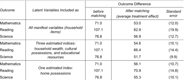
We conducted the propensity score matching three times, to see how results are affected by including the estimated latent variable instead of a set of manifest variables. First, we included all the manifest variables in the list of matching covariates. More precisely, we included all dummy variables denoting household items. Second, we included three indices estimated from the manifest variables and reflecting three latent variables: household wealth, household cultural possessions and household educational resources. Finally, we estimated only one latent variable using all manifest variables and reflecting all possible home possessions. We expected that the first approach would differ from the second in terms of precision of the estimates of the average treatment effect. More precisely, we expected that the second approach would provide estimates with smaller standard errors, in line with the theory and simulation results presented above. Furthermore, we expected that the third approach, based on only one latent variable instead of three, could be less efficient, as restricting a latent dimension to one limits the amount of relevant information provided in matching if there are, in fact, three distinct latent variables behind the values of the manifest variables. This example demonstrates typical problems that arise in empirical research: first, whether to estimate the latent trait instead of using manifest variables directly in matching; and second, how many latent variables should be estimated.

(20)

Table 6 presents results for this empirical exercise. First, note that the differences in outcomes go down after matching. We expected that, as differences in outcomes between different types of schools are driven mainly by differences in student characteristics. However, the outcomes differences remain quite large and in favor of general-vocational schools, even after adjusting for intake scores, gender, parents’ education and occupation, and family resources. The average treatment effects vary across the sets of results, with the biggest gap being found in reading and slight differences across matching methods, but we are mainly interested in the magnitude of standard errors. More precisely, we want to see how standard errors change when matching is conducted directly on manifest variables and when matching uses the estimated indices.

Table 6. Empirical example: achievement difference between general-vocational and vocational schools

Outcome Latent Variables Included as

Outcome Difference

before matching

After matching (average treatment effect)

Standard error

Mathematics

All manifest variables (household items)

71.0 53.0 (12.0)

Reading 107.1 62.9 (19.9)

Science 76.8 56.9 (12.7)

Mathematics Three estimated indices:

household wealth, cultural possessions, and educational

resources

71.0 54.6 (10.1)

Reading 107.1 66.4 (14.4)

Science 76.8 51.7 (9.9)

Mathematics

One estimated index: home possessions

71.0 56.1 (10.7)

Reading 107.1 70.9 (14.8)

Science 76.8 55.3 (10.1)

Notes: Number of treated: 461; Number of controls: 607; Standard errors obtained by bootstrapping and adjusted for clustering at the school level

The results demonstrate the benefits of using the estimated latent variables in matching. While the average treatment effects are reasonably similar across matching methods, the standard errors are 20–40% higher for matching conducted on the manifest variables. The results are quite similar for matching on the three estimated latent variables and for matching on the one estimated variable. Standard errors are slightly higher when matching on only one instead of on three latent variables, which suggests that our data have three-dimensional latent structure. However, standard errors are also much lower in this case, compared to matching directly on all manifest variables.

This example confirms our main findings from the simulation study. Clear benefits are gained from matching on the estimated latent variables rather than on the set of manifest variables, at least with moderate sample sizes and a well-developed latent variables framework. Matching on the three estimated latent variables substantially lowered standard

(21)

errors of the treatment effects. Matching on the one latent variable gave similar results, which were still clearly better than those obtained with matching directly on the manifest variables.

V. Summary

This paper demonstrates how modeling and including the latent variable in the propensity score matching can improve the quality of the treatment estimates in comparison to the more standard approach when matching is conducted directly on the set of manifest variables, even if they reflect the same latent trait. Our simple theory explains how including the estimated latent variable can limit the measurement error in estimating the propensity score that is introduced by a noisy signal contained in the manifest variables. We present simulation studies demonstrating the range of efficiency gains from incorporating the latent variable in matching. And, we apply these to real educational data, showing the importance of our findings through this empirical example.

We find, generally, that estimating the latent variable and using this estimate for propensity score matching lowers the variance of the average treatment estimators. The variance is seemingly smaller with small and moderate sample sizes, but the benefits are still visible even for large samples. Using the estimated latent variable rather than matching directly on a set of manifest variables is always preferable in small sample sizes with a large number of manifest variables available, with manifest variables containing a strong signal about the latent variable and when outcome-generating process is non-linear in the latent variable. Efficiency increases much more for the nearest neighbor matching than for the local linear regression matching. We argue that, in the latter case, using many control variables to estimate the control outcome for each treated limits the deteriorating impact of measurement error. However, with this method the variance is also visibly lower when matching on the estimated latent variable.

Our final advice is to follow our three-step strategy: estimate the latent variable using observed manifest variables; use this estimate to estimate the propensity score; and match on this propensity score to estimate the average treatment effects. However, this is advisable only in cases where we have a strong theory on how the observed manifest variables relate to each other and to the latent construct, and how the latent construct relates to outcomes and to the selection process. Without a sound theory, such an approach could be misleading, as the estimated latent variables can contain irrelevant information and can even bias the average treatment effects. If such a theory exists and can be confirmed empirically, applying our approach to observational data is usually highly desirable.

(22)

References

Abbring, J. H. and J. J. Heckman (2007). “Econometric Evaluation of Social Programs, Part III: Distributional Treatment Effects, Dynamic Treatment Effects, Dynamic Discrete Choice, and General Equilibrium Policy Evaluation,“ in: J.J. Heckman and E.E. Leamer (Ed.), Handbook of Econometrics, Vol. 6, Chapter 72. Amsterdam: Elsevier. Agodini R. and M. Dynarski (2004). “Are Experiments the Only Option? A Look at Dropout

Prevention Programs,“ The Review of Economics and Statistics, 86(1), pp. 180–194. Frölich M. (2004), “Finite-Sample Properties of Propensity-Score Matching and Weighting

Estimators,“ The Reviewof Economics and Statistics, 86(1), pp. 77–90.

Heckman, J.J., H. Ichimura and P.E. Todd (1998), “Matching as an Econometric Evaluation Estimator”, Review of Economic Studies 65, pp. 261–294.

Jakubowski M., Patrinos H. A., Porta E. E., and Wiśniewski J. (2010), “The Impact of the 1999 Education Reform in Poland”, Policy Research Working Paper Series 5263, The World Bank.

Jakubowski M. and A. Pokropek (2009), “Family income or knowledge? Decomposing the impact of socio-economic status on student outcomes and selection into different types of schooling”, paper presented at the PISA Research Conference, September 2009, Kiel (Germany).

Jalan J. and M. Ravallion, (2003). “Estimating the Benefit Incidence of an Antipoverty Program by Propensity-Score Matching,” Journal of Business & Economic

Statistics, American Statistical Association, 21(1), January, pp. 19–30.

Joreskog, K. G. (1971). “Statistical analysis of sets of congeneric tests,” Psychometrika, 36, pp. 109–132.

OECD (2007), PISA 2006 Science Competencies for Tomorrow’s World, OECD, Paris. OECD (2009), PISA 2006 Technical Report, OECD, Paris.

Rosenbaum, P.R. and D.B. Rubin (1983), “The Central Role of the Propensity Score in Observational Studies for Causal Effects”, Biometrika 70(1), pp. 41–55.

Rubin, D. (1973), “Matching to Remove Bias in Observational Studies,” Biometrics, 29 (March 1973), pp. 159–183.

Skrondal, A. and S. Rabe-Hesketh (2004), Generalized Latent Variable Modeling: Multilevel,

Longitudinal and Structural Equation Models. Boca Raton, FL: Chapman &

Hall/CRC.

Smith J. A. and P. E. Todd (2005). “Does matching overcome LaLonde's critique of nonexperimental estimators?,” Journal of Econometrics, 125(1-2), pp. 305–353. White M. and J. Killeen (2002). “The Effect of Careers Guidance for Employed Adults on

Continuing Education: Assessing the Importance of Attitudinal Information”,

Journal of the Royal Statistical Society. Series A (Statistics in Society), 165(1), pp.

(23)

Appendix A. Additional Results for Simulation Study

Table A1. Basic Statistics: random sample from Simulation A*

Quasi-experimental group

Stats _VariableLatent Manifest Variables _{Latent Score}Estimated Outcome

m1 m2 m3 m4 m5

Controls mean -0.003 -0.025 -0.462 0.075 0.065 -0.109 -0.003 -10.113 SD 1.032 5.244 4.997 5.082 5.000 5.081 0.360 5.238 Treated mean -0.029 -0.061 0.291 0.071 -0.231 0.261 0.006 -7.113 SD 0.888 4.441 4.846 5.068 5.274 4.787 0.362 4.620

*Note: (500 observations, 5 manifest variables, signal-to-noise ratio 1:1)

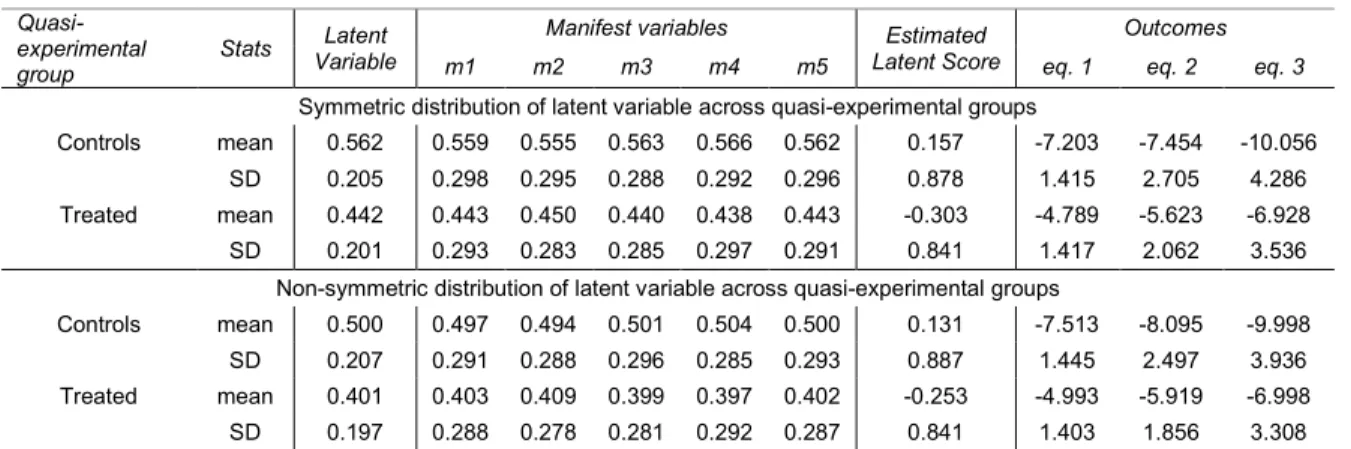
Table A2. Basic statistics: random sample from simulation B*

Quasi-experimental group

Stats Latent

Variable

Manifest variables _Estimated

Latent Score

Outcomes

m1 m2 m3 m4 m5 eq. 1 eq. 2 eq. 3

Symmetric distribution of latent variable across quasi-experimental groups

Controls mean 0.562 0.559 0.555 0.563 0.566 0.562 0.157 -7.203 -7.454 -10.056 SD 0.205 0.298 0.295 0.288 0.292 0.296 0.878 1.415 2.705 4.286 Treated mean 0.442 0.443 0.450 0.440 0.438 0.443 -0.303 -4.789 -5.623 -6.928 SD 0.201 0.293 0.283 0.285 0.297 0.291 0.841 1.417 2.062 3.536

Non-symmetric distribution of latent variable across quasi-experimental groups

Controls mean 0.500 0.497 0.494 0.501 0.504 0.500 0.131 -7.513 -8.095 -9.998 SD 0.207 0.291 0.288 0.296 0.285 0.293 0.887 1.445 2.497 3.936 Treated mean 0.401 0.403 0.409 0.399 0.397 0.402 -0.253 -4.993 -5.919 -6.998 SD 0.197 0.288 0.278 0.281 0.292 0.287 0.841 1.403 1.856 3.308

(24)

Table A3. Mean estimate of the average treatment effect

nearest neighbor local linear regression Sample

size latent manifest estimated latent latent manifest estimated latent latent manifest estimated latent Symmetric distributions of latent variables

Equation 1 500 3.000 2.883 2.882 2.998 2.879 2.882 2.998 2.878 2.882 5000 3.000 2.882 2.882 3.000 2.883 2.884 3.000 2.882 2.883 Equation 2 500 3.057 2.819 2.817 3.000 2.800 2.801 2.998 2.799 2.800 5000 3.058 2.819 2.819 3.000 2.802 2.802 2.997 2.801 2.801 Equation 3 500 3.005 2.997 2.997 3.003 2.994 2.994 3.014 2.994 2.999 5000 3.008 3.000 3.001 3.000 2.996 2.997 3.002 3.001 3.003

Non-symmetric distributions of latent variables

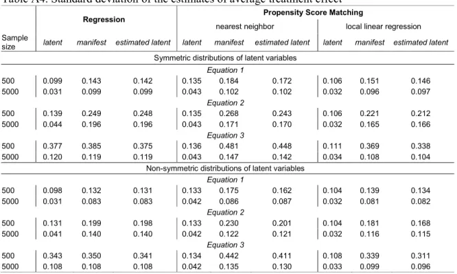
Table A4. Standard deviation of the estimates of average treatment effect

nearest neighbor local linear regression Sample

size latent manifest estimated latent latent manifest estimated latent latent manifest estimated latent Symmetric distributions of latent variables

Non-symmetric distributions of latent variables