NUMERICAL SIMULATIONS OF DIE CASTING WITH UNCERTAINTY QUANTIFICATION AND OPTIMIZATION USING NEURAL NETWORKS
BY
SHANTANU SHASHANK SHAHANE
DISSERTATION
Submitted in partial fulfillment of the requirements
for the degree of Doctor of Philosophy in Mechanical Science and Engineering in the Graduate College of the
University of Illinois at Urbana-Champaign, 2019
Urbana, Illinois
Doctoral Committee:
Professor Narayana R. Aluru, Chair
Professor Surya Pratap Vanka, Director of Research Professor Shiv Gopal Kapoor, Director of Research Professor Placid Ferreira
Professor Arif Masud
Abstract
Die casting is one type of metal casting in which liquid metal is solidified in a reusable die. In such a complex process, measuring and controlling the process parameters is dif-ficult. Conventional deterministic simulations are insufficient to completely estimate the effect of stochastic variation in the process parameters on product quality. In this research, a framework to simulate the effect of stochastic variation together with verification, val-idation, uncertainty quantification and design optimization is proposed. This framework includes high-speed numerical simulations of solidification, micro-structure and mechanical properties prediction models along with experimental inputs for calibration and validation. In order to have a better prediction of product quality, both experimental data and stochas-tic variations in process parameters with numerical modeling are employed. This enhances the utility of traditional numerical simulations used in die casting.
OpenCast, a novel and comprehensive computational framework to simulate solidifica-tion problems in materials processing is developed. Heat transfer, solidificasolidifica-tion and fluid flow due to natural convection are modeled. Empirical relations are used to estimate the microstructure parameters and mechanical properties. The fractional step algorithm is mod-ified to deal with the numerical aspects of solidification by suitably altering the coefficients in the discretized equation to simulate selectively only in the liquid and mushy zones. This brings significant computational speed up as the simulation proceeds. Complex domains are represented by unstructured hexahedral elements. The algebraic multigrid method, blended with a Krylov subspace solver is used to accelerate convergence.
chaos expansion (PCE) and neural network with OpenCast for uncertainty quantification and optimization. The effects of stochasticity in the alloy composition, boundary and initial conditions on the product quality of die casting are analyzed using PCE. Further, a high dimensional stochastic analysis of the natural convection problem is presented to model uncertainty in the material properties and boundary conditions using neural networks. In die casting, heat extraction from molten metal is achieved by cooling lines in the die which impose nonuniform boundary temperatures on the mold wall. This boundary condition along with the initial molten metal temperature affect the product quality quantified in terms of micro-structure parameters and yield strength. Thus, a multi-objective optimization problem is solved to demonstrate a procedure for improvement of product quality and process efficiency.
Acknowledgments
This research would not have been possible without the guidance of my advisers Prof. Surya Pratap Vanka, Prof. Narayana Aluru, Prof. Shiv Kapoor and Prof. Placid Ferreira. Since this project involved interdisciplinary work, I got a rare opportunity of working with above four professors who have expertise in different fields. I would like to specially thank Prof. Vanka for supporting me during the development of the numerical software which I think was one of the tough phases of my doctoral research. I express deepest gratitude towards Digital Manufacturing and Design Innovation Institute - UI Labs for funding this project (award: DMDII 15–07–06). Steve Udvardy and Beau Glim from the North American Die Casting Association (NADCA) helped in setting up contacts with multiple die casting industries which shared experimental data useful in this research. I am grateful to Alex Monroe from Mercury Castings for insightful suggestions regarding the die casting process. Finally, I would like to thank my parents and numerous friends for their support.
Table of Contents
List of Tables . . . ix
List of Figures . . . x
Chapter 1 Introduction . . . 1
1.1 Virtual Certification Framework . . . 3
1.2 Objectives of the Research . . . 5
1.3 Thesis Outline. . . 6
Chapter 2 Description of Deterministic Numerical Model . . . 9
2.1 Introduction . . . 9
2.2 Governing Equations . . . 11
2.3 Solution Algorithm . . . 13
2.4 Discretization on an Unstructured Grid . . . 15
2.5 Special Modifications in Solidification Regions . . . 18
2.5.1 Momentum equation . . . 19
2.5.2 Pressure Poisson Equation . . . 20
2.5.3 Face Volume Flux Computation and Velocity Correction . . . 22
2.5.4 Latent Heat Term . . . 23
2.6 Solver for Linear Systems . . . 26
2.7 Grain Growth and Mechanical Properties Models . . . 28
Chapter 3 Parameter Uncertainty Quantification . . . 30
3.1 Introduction . . . 30
3.2 Polynomial Chaos Expansion . . . 32
3.3 Deep Neural Network . . . 35
Chapter 4 Verification and Validation . . . 38
4.1 Verification . . . 38
4.2 Validation . . . 41
Chapter 5 Deterministic Solidification Results of Realistic Geometries . 47 5.1 Geometry and Mesh . . . 47
5.2 Effect of Natural Convection . . . 51
5.2.2 Connector Rib. . . 55
5.3 Solid Fraction and Temperature . . . 57
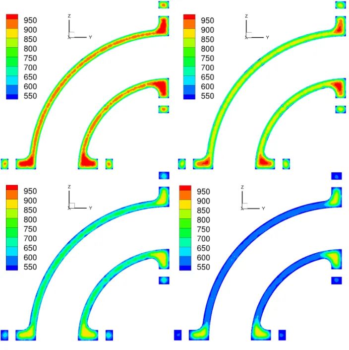
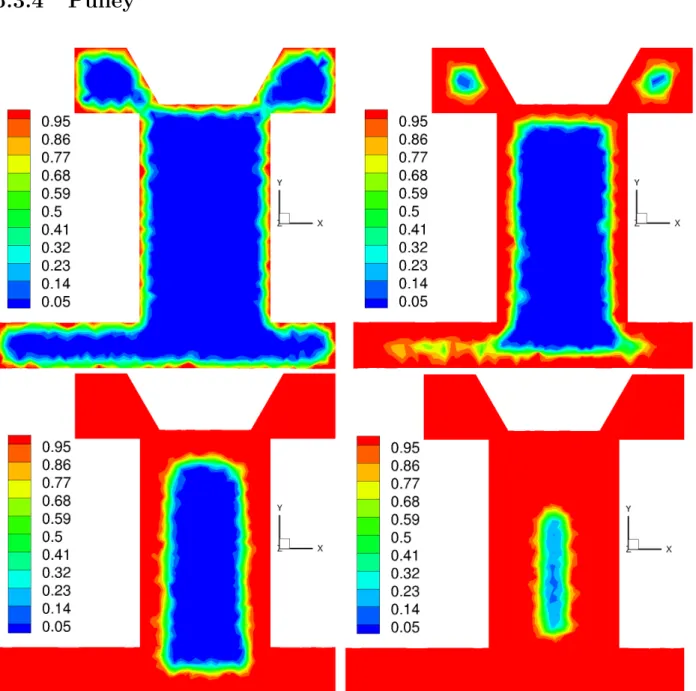
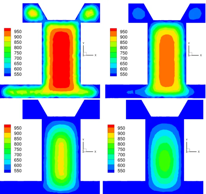
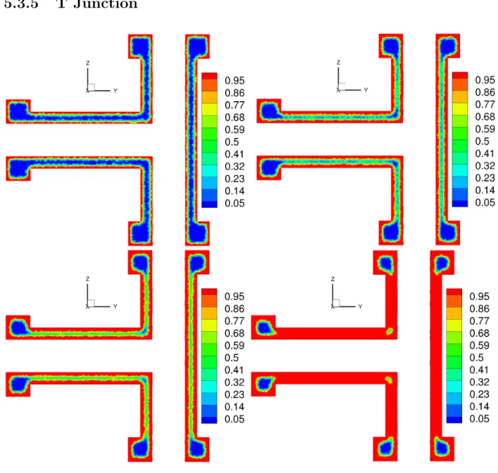
5.3.1 Clamp . . . 57 5.3.2 Connector Rib. . . 58 5.3.3 Elbow Pipe . . . 59 5.3.4 Pulley . . . 61 5.3.5 T Junction . . . 63 5.3.6 Disc . . . 65
5.4 Microstructure and Yield Strength . . . 66
5.4.1 Elbow Pipe . . . 68 5.4.2 Tub . . . 69 5.4.3 Pulley . . . 70 5.4.4 T Junction . . . 71 5.4.5 Disc . . . 72 5.5 Conclusions . . . 73
Chapter 6 Uncertainty Quantification in Three Dimensional Natural Con-vection . . . 75
6.1 Introduction . . . 76
6.2 Grid Independence Study . . . 80
6.3 Deterministic Results: Output Values at Input Mean . . . 81
6.4 Description of Cases A and B . . . 83
6.5 Case A Results . . . 86
6.5.1 Stochastic Convergence . . . 87
6.5.2 Nusselt Number . . . 88
6.5.3 Velocity and Temperature . . . 91
6.5.4 Sensitivity Analysis . . . 95
6.6 Case B Results . . . 96
6.6.1 Deep Neural Network Training and Testing. . . 96
6.6.2 Nusselt Number . . . 100
6.6.3 Velocity and Temperature . . . 102
6.7 Conclusions . . . 107
Chapter 7 Uncertainty Quantification Applied to Solidification Problems 109 7.1 Connector Rib. . . 109
7.1.1 Linear Temperature Solid Fraction Relation . . . 109
7.1.2 Nonlinear Temperature Solid Fraction Relation . . . 112
7.2 Clamp . . . 115
7.2.1 Stochastic Convergence . . . 118
7.2.2 Results. . . 121
Chapter 8 Optimization of Solidification Process . . . 126
8.1 Introduction . . . 126
8.2 Formulation of Optimization Problem . . . 128
8.3 Genetic Algorithm . . . 131
8.3.1 Single Objective Optimization . . . 131
8.3.2 Multi-Objective Optimization . . . 133
8.3.3 Neural Network . . . 134
8.4 Assessment of Genetic Algorithm on Simpler Problems . . . 136
8.4.1 Single Objective Optimization . . . 137
8.4.2 Bi-Objective Optimization . . . 139
8.5 Results of Multi-Objective Optimization Problem with Eleven Inputs . . . . 143
8.6 Conclusions . . . 146
Chapter 9 Conclusions . . . 148
9.1 OpenCast: Numerical Software . . . 148
9.2 Parameter Uncertainty Quantification and Sensitivity Analysis . . . 149
9.3 Design Optimization . . . 151
9.4 Recommendation for Future Studies . . . 152
List of Tables
4.1 Stochastic Collocation Convergence Analysis . . . 45
5.1 Clamp Geometry: Comparison With and Without Natural Convection . . . 52
6.1 Stochastic Collocation Error Analysis . . . 88
6.2 Relative Average Percent Error: DNN Training and Testing . . . 100
6.3 Shift of Mean Relative to Deterministic Values . . . 108
7.1 Stochastic Collocation Error Estimate. . . 110
7.2 Stochastic Collocation Error Estimate. . . 113
7.3 Stochastic Collocation Convergence Analysis . . . 119
7.4 Clamp Geometry: Grid Independence . . . 121
8.1 Neural Network Parameters, Training and Testing Errors . . . 135
8.2 Single Objective Optimization: Genetic Algorithm Estimates compared with Parameter Sweep Values for Two Input Problems . . . 139
List of Figures
1.1 Die Casting Assembly Schematic . . . 2
1.2 Virtual Certification Framework . . . 3
2.1 Unstructured Hexahedral Control Volumes . . . 16
2.2 Control Volumes with Solid Liquid Interface . . . 19
2.3 Solid Fraction Temperature Relation . . . 25
2.4 Disjoint Regions near the End of Solidification . . . 28
3.1 Neural Network Schematics . . . 36
4.1 Differentially Heated Cube Schematic . . . 38
4.2 Temperature Profiles (Ra= 105) . . . . 40
4.3 Velocity Profiles (Ra= 105) . . . 40
4.4 Velocity Profiles (Ra= 106) . . . . 41
4.5 Temperature-Time Plot for Cooling Rate 5 K/min. . . 42
4.6 Experimental and Simulated Temperatures with Error Bounds . . . 46
5.1 A Representative Clamp Geometry . . . 48
5.2 A Typical Connector Rib . . . 48
5.3 Elbow Pipe . . . 49 5.4 Tub . . . 49 5.5 Pulley . . . 50 5.6 T Junction. . . 50 5.7 Disc . . . 51 5.8 Clamp: SDAS (µm) . . . 53
5.9 Clamp: Grain Size (µm) . . . 53
5.10 Clamp: Yield Strength (MPa) . . . 54
5.11 Clamp: Local Solidification Time (s) . . . 54
5.12 Connector Rib: SDAS (µm) . . . 55
5.13 Connector Rib: Grain Size (µm) . . . 55
5.14 Connector Rib: Yield Strength (MPa) . . . 56
5.15 Connector Rib: Local Solidification Time (s) . . . 56
5.16 Clamp: Temperature Contours with Time (K) . . . 57
5.17 Clamp: Solid Fraction Contours with Time . . . 57
5.19 Elbow Pipe: Solid Fraction Contours with Time . . . 59
5.20 Elbow Pipe: Temperature Contours with Time . . . 60
5.21 Pulley: Solid Fraction Contours with Time . . . 61
5.22 Pulley: Temperature Contours with Time . . . 62
5.23 T Junction: Solid Fraction Contours with Time . . . 63
5.24 T Junction: Temperature Contours with Time . . . 64
5.25 Disc: Solid Fraction Contours with Time . . . 65
5.26 Disc: Temperature Contours with Time . . . 66
5.27 Elbow Pipe . . . 68 5.28 Tub . . . 69 5.29 Pulley . . . 70 5.30 T Junction . . . 71 5.31 Disc XY Cross-section . . . 72 5.32 Disc YZ Cross-section . . . 73
6.1 Temperature and Velocity Contours for Ra= 105 . . . 80
6.2 Temperature and Velocity Contours for Ra= 106 . . . . 81
6.3 Deterministic Results for Ra= 105 and P r= 7.5 . . . . 82
6.4 Deterministic Results for Ra= 106 and P r= 7.5 . . . 83
6.5 Samples of Temperature Boundary Condition . . . 86
6.6 Mean Nusselt Number Estimate from Numerical Simulation and Polynomial Chaos Expansion . . . 88
6.7 Spatial Mean Nusselt Number Response Surface . . . 89
6.8 Local Nusselt Number at Hot Wall for Ra= 105 . . . . 90
6.9 Local Nusselt Number at Hot Wall for Ra= 106 . . . 90
6.10 Temperature at Z = 0.5 Mid-plane for Ra= 105 . . . . 91
6.11 X Velocity at Z = 0.5 Mid-plane forRa= 105 . . . . 92
6.12 Y Velocity at Z = 0.5 Mid-plane forRa= 105 . . . 93
6.13 Temperature at Z = 0.5 Mid-plane for Ra= 106 . . . . 93
6.14 X Velocity at Z = 0.5 Mid-plane forRa= 106 . . . . 94
6.15 Y Velocity at Z = 0.5 Mid-plane forRa= 106 . . . 94
6.16 Sensitivity: 6 Outputs, 2 Inputs . . . 95
6.17 DNN Training and Validation Loss for 4 Strips . . . 98
6.18 Estimate from Numerical Simulation and DNN for 4 Strips . . . 99
6.19 Ra= 106Hot Wall Nusselt Number: Difference between Stochastic Mean and Deterministic Value . . . 101
6.20 Ra= 106 Hot Wall Nusselt Number: Stochastic Standard Deviation . . . 102
6.21 Ra= 106 Z Midplane Temperature: Difference between Stochastic Mean and Deterministic Value . . . 104
6.22 Ra = 106 Z Midplane X-Velocity: Difference between Stochastic Mean and Deterministic Value . . . 105
6.23 Ra = 106 Z Midplane Y-Velocity: Difference between Stochastic Mean and Deterministic Value . . . 106
7.1 Connector Rib: Response Surfaces. . . 112
7.2 Connector Rib: Response Surfaces. . . 114
7.3 Al–Si Phase Diagram [1] . . . 117
7.4 Polynomial Chaos and Numerical Simulation Estimates (Non-dimensionalized)120 7.5 Sensitivity of 4 Outputs to 3 Inputs . . . 122
7.6 Response Surfaces. . . 123
7.7 Probability Density Functions . . . 124
8.1 Boundary Condition Representation by Domain Decomposition . . . 129
8.2 Clamp Temperature Contours (K) (Solidification Time: 3.02 s). . . 130
8.3 Clamp Solid Fraction Contours (Solidification Time: 3.02 s) . . . 130
8.4 Clamp Microstructure Parameters . . . 131
8.5 Neural Networks: Error Estimates for 200 Testing Samples . . . 136
8.6 Parameter Sweep: Uniform Boundary Temperature . . . 137
8.7 Parameter Sweep: Split Boundary Temperature with Tinit = 1000 K . . . 138
8.8 Uniform Boundary Temperature: Solidification Time v/s Min. Yield Str. . . 140
8.9 Uniform Boundary Temperature: Max. Grain Size v/s Min. Yield Str. . . . 140
8.10 Split Boundary Temperature with Tinit = 1000 K: Solidification Time v/s Min. Yield Str. . . 141
8.11 Split Boundary Temperature with Tinit = 1000 K: Max. Grain Size v/s Min. Yield Str. . . 142
8.12 Pareto Front . . . 143
8.13 Local Sensitivity for Designs on Pareto Front . . . 144
8.14 Pareto Front for 3 Objectives . . . 145
Chapter 1
Introduction
A variety of processes are used in the manufacturing industry to produce a finished product. These processes are quite complex in nature and demand high conformity to tolerances. Due to recent advances in computing hardware and software it is possible to simulate the physics of the process using numerical simulations. These simulations map the input to output process parameters and thus can be used to estimate the final product quality. Development of real-time data acquisition systems has facilitated the measurement of parameters during physical experiments. In order to increase the simulation accuracy, there is a need to couple experimental data with numerical simulations. Moreover in the industrial environment, controlling the process parameters tightly is often costly and time consuming. Thus, there is substantial stochastic variation in the process parameters. Traditional numerical simulation techniques are unable to predict the effect of this variation on the product quality. Therefore, the aim of this research is to combine experimental data and stochastic variations with numerical simulations and thus, increase the confidence in simulations. Simulations are financially viable and less time consuming and hence, can be used as proxies to actual experiments. Several complex processes involving a large number of process parameters affect the final product quality. Due to recent advances in computing hardware and software, it is now possible to simulate the physics of these processes using numerical simulations. These simulations provide detailed flow and temperature histories and can be used to estimate the final product quality. Frequently, it is difficult to measure and tightly control all the process parameters. However, they can have a significant impact on the process as well as the predicted product strength.
Die casting is an important manufacturing process used when high production rates and complex geometries are required to be manufactured. Figure 1.1 shows a typical schematic of the die assembly. The die is generally made out of steel consisting of two halves which are separated along the parting line and held in place by multiple ejector pins. Cooling lines are designed in the die to flow a coolant, typically water. The mold cavity is sprayed with a lubricant which helps to control the die temperature and also reduces the sticking of the molten metal to the die during the removal. Then, the two die halves are closed and liquid metal is filled in the cavity. The flowing coolant maintains temperature of the die and extracts heat from the molten metal. After solidification, the two halves are separated by sliding along the ejector pins. The last step is shakeout in which the scrap (gates, runners etc.) are separated from the casting and the casting is further cooled to room temperature either by quenching in water or leaving open to air. Cycle times vary from a couple of seconds for small components weighing less than one ounce, to thirty seconds for a casting of several pounds. Aluminum, magnesium and zinc alloys are the most popular materials used in die casting. Die cast products are more commonly used in automotive and housing industries.
1.1
Virtual Certification Framework
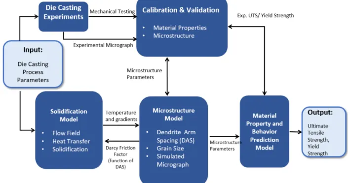
Individual components of virtual certification framework are shown in fig. 1.2. The top and bottom links connect the input process parameters to outputs using experiments and numerical simulations, respectively. Real life die castings are used to calibrate the empirical models for microstructure and material property parameters. Temperature gradients and cooling rates estimated using the numerical simulations are inputs to these models. The numerical software is verified using published results for canonical problems and validated using the experimental results. Uncertainty quantification is a wrapper on the deterministic software in order to estimate the impact of stochastic variation in the process parameters on the final product quality. Here, each module of the framework (fig. 1.2) is described briefly.
Figure 1.2: Virtual Certification Framework
As depicted in Fig. 1.2, the major outcome of the virtual certification methodology is the predictive framework that provides properties and behavior of die-cast materials under various conditions. Experimental validation establishes the accuracy of using
mathemati-cal models, uncertainties, and numerimathemati-cal simulation approaches for simulating die casting manufacturing processes. Experimental data on a variety of real-life die casting parts from the industry are obtained for the validation. Initially, a part of the experimental data is used to compare the model predictions and improvements in the computational models are made, if necessary as a calibration step. The calibration experimental data serves as a useful platform to improve computational models. After ensuring the computational results match with the calibration experimental data, the computational models are further tested with the remaining experimental data, i.e., data that is not used as part of the calibration process. This two-step procedure ensures rigorous validation.
Temperature evolution and velocity distribution during solidification of pure metals and metal alloys has been analyzed by many researchers [2–11]. Some of the common numerical approaches include continuum mixture model [2,3], enthalpy method [4], Lattice Boltzmann method [8] and smoothed particle hydrodynamics [9]. Some researchers have implemented analytical solutions using scaling analysis or asymptotic methods on simple geometries [5, 7]. Temperature distribution and flow patterns during experimental solidification of pure metals or binary alloys are useful for calibration and validation [10–12]. Quillet et al. [10] and Hachani et al. [11] reported the temperature distribution and macro-segregation of solute with an experimental solidification of a Tin based alloy in an ingot. Solidification phenomena of die casting involves interplay between heat transfer and flow due to natural convection. All the references discussed above simulated solidification in rectangular or cuboidal geometries and hence, structured Cartesian grids were used. Practical die casting geometries are complex and thus, unstructured hexahedral elements are utilized in this work. Multiple algorithms are discussed in the literature to simulate fluid flow on unstructured grids [13–18]. Discretization strategy implemented in this research is an extension of the work by Mathur and Murthy [17] and Muzaferija and Gosman [18].
For die casting, the microstructure parameters like grain size and dendritic arm spacing are important as they affect the final product quality. Phase field modeling [19–21] is a
popular method used to study the evolution of the microstructure during solidification. The phase field method simulates the growth of each dendrite and thus, it is computationally expensive at the length scale of die cast products. In this research, an empirical relation from the work of Backer and Wang [22] is used to estimate secondary dendritic arm spacing. There are various models [23–25] suggested for grain size estimation during solidification. Here, the isothermal crystal growth model [24] is used.
Use of deterministic simulations alone to analyze the engineering systems is incomplete due to the lack of precisely defined input data. Thus, there has been a growing interest [26–35] in coupling uncertainty propagation techniques with the deterministic numerical simulations to estimate the effects of stochastic variations in the input process parameters on the outputs. The polynomial chaos expansion is a popular method used to estimate the relation between input and output parameters. Stochastic Galerkin projection [26–28] and collocation [29–31] are two strategies to estimate the coefficients of the polynomial chaos expansion. Stochastic Galerkin method is an intrusive method since it requires solution of a new set of equations and thus, modification of the underlying deterministic code which becomes a significant additional effort. Hence, recently non-intrusive stochastic collocation methods have been developed which need multiple evaluations of the deterministic simula-tion at predefined collocasimula-tion points obtained by sampling from the probability distribusimula-tion function of the input parameters. Values of outputs estimated at these samples are then used to estimate the coefficients of the polynomial chaos expansion.
1.2
Objectives of the Research
Simulating a die casting process requires developing predictive models involving multiple physical phenomena such as solidification, fluid flow and heat transfer, defining various un-certainties in process parameters and then developing a solution algorithm. However, despite the high power of numerical algorithms and the availability of extensive property data,
con-siderable uncertainties and errors exist in the current day simulation techniques. In addition, gaps in the knowledge base also exist, especially in the interaction of material microstruc-ture with physical property fluctuations. Therefore, in order to obtain a comprehensive tool for accurately predicting quality of the die casting products, a virtually guided certification methodology has been developed. Virtually guided certification aims to increase the accu-racy of numerical simulations using a framework connecting experimental data, predictive models and uncertainty quantification. The present effort aims to reduce the uncertainty in the numerical simulation results through verification, validation and uncertainty quantifica-tion. Accurate prediction of outputs with error bars can reduce scrap castings thus, giving monetary benefits.
The main objective of this work is to incorporate the effects of the stochastic variation in the process parameters of die casting in the numerical simulation. An in-house numerical software OpenCast is developed using finite volume method to simulate the solidification process along with fluid flow due to natural convection and heat transfer. The temperature gradients and cooling rates are used to estimate the micro-structure parameters like grain size and mechanical properties like yield strength. Verification and validation is done by published numerical and experimental results. Uncertainty quantification is used to assess the impact of stochasticity in the input parameters on the output parameters. Further, optimal boundary temperature distribution is estimated in order to improve productivity and quality of the casting. Thus, a framework with calibration, verification, validation, uncertainty quantification and design optimization coupled to numerical simulation has been developed.
1.3
Thesis Outline
Outline of the thesis is as follows:
discusses special considerations required for the solidification problems like coefficient modification and nonlinear solid fraction temperature relation. It ends with description of the empirical microstructure and mechanical properties models.
Chapter 3 begins with the literature survey of use of uncertainty quantification and its utility. Then it describes the polynomial chaos expansion method and deep neural networks which are used as surrogate models.
Chapter 4 presents the verification using the published numerical natural convection results. Validation is done with published experimental results of solidification. This chapter emphasizes the need of incorporating stochasticity in the validation.
Chapter 5 demonstrates the application of the software on solidification of multiple practical casting geometries. Plots of solid fraction, temperature, microstructure and mechanical properties are included. This chapter also talks about the effect of natural convection in casting simulation.
Chapter 6 presents the results of parameter uncertainty and sensitivity analysis for a natural convection problem. The polynomial chaos and neural network methods discussed in chapter 3 are used for low and high dimensional stochastic analysis re-spectively.
Chapter 7 presents the parameter uncertainty and sensitivity analysis on multiple casting problems. A detailed discussion about the effect of stochasticity in the inputs like boundary condition, initial condition and material properties on the outputs like solidification time, microstructure and mechanical properties is included.
Chapter 8 discusses the results of multi-objective optimization of solidification of a particular casting geometry. A genetic algorithm is coupled with a deep neural network as a surrogate model. Initial and boundary temperature distributions are estimated
in order to optimize the productivity and casting quality. Finally, a local sensitivity analysis is used to rank the multiple optimal designs and identify the best design. Chapter 9 concludes with the results and the key achievements of this dissertation.
Chapter 2
Description of Deterministic
Numerical Model
2.1
Introduction
Temperature evolution and velocity distribution during solidification of pure metals and metal alloys has been analyzed by many researchers. Bennon and Incropera [2] used a continuum mixture model to solve the momentum and energy equations and applied it to the solidification problem of a rectangular cavity filled with a binary aqueous solution [3]. From their work, it is clear that although the continuum formulation has a limitation of smearing the interface, it is efficient than the multiple region method in which the governing equations are solved in each phase separately with appropriate interface conditions. Implementing multiple region method for a practical complex geometry with irregular interfaces is quite difficult and computationally expensive. Voller and Prakash [4] used the Darcy’s law of drag and the enthalpy method to model the mushy zone during solidification of a square cavity. Two vertical walls were held at below and above the melting point and the horizontal walls were thermally insulated. The damping of velocities in the mushy zone due to Darcy’s law is clearly seen in the velocity vector plot. Vynnycky and Kimura [5] solved a similar problem in a rectangular enclosure analytically. They used an asymptotic approach to solve the non-dimensional momentum and energy equations for the case of the Rayleigh and Stefan numbers much larger and smaller than unity, respectively. Comparison with finite element transient numerical simulation showed that such an asymptotic simplification is possible. Bennett [6] used adaptive grid with local rectangular refinement (LRR) to model solidification with fluid flow in multiple rectangular geometries. The adaptive LRR grid
needed half the storage and computational effort compared to the non-adaptive grid. Wang et al. [36] discussed a numerical model for melting in a rectangular cavity with natural convection at high Rayleigh number (108). They used the consistent update technique (CUT) algorithm with a multigrid solver. Plotkowski et al. [7] simulated analytically and numerically heat transfer and fluid flow for solidification in a rectangular cavity. They used scaling analysis to simplify the governing equations of the mixture model followed by an analytical solution and comparison with a finite volume solution for an Al-Cu binary alloy. Hu et al. [8] studied the three-dimensional phase change problem with natural convection using the Lattice Boltzmann method. They simulated melting in a cubical cavity and in cavities with inner rectangular cylinders and sphere. Cleary et al. [9] used smoothed particle hydrodynamics to model filling and solidification in high pressure die casting. They simulated practical industrial case studies like differential cover, an electronic housing and a door lock plate. Gau and Viskanta [12] performed experiments to understand the importance of natural convection during solidification and melting of pure metal. Quillet et al. [10] and Hachani et al. [11] reported the temperature distribution and macro-segregation of solute with an experimental solidification of a Tin based alloy in an ingot. Such experimental work is useful for calibration and validation of the numerical methods.
Solidification phenomena of die casting involves interplay between heat transfer and flow due to natural convection. All the references discussed above simulated solidification on rectangular or cuboidal geometries and hence, structured Cartesian grids were used. Practical die casting geometries are complex and thus, unstructured hexahedral elements are utilized in this work. Multiple algorithms are discussed in the literature to simulate fluid flow on unstructured grids [13–18]. Discretization strategy implemented in this research is an extension of the work by Mathur and Murthy [17] and Muzaferija and Gosman [18]. Solution of the fluid flow and the pressure Poisson equation involves a significant computational effort. As the solidification problem proceeds, the volume of liquid zone deceases continuously and it is not necessary to solve for fluid flow in the solid zone. We therefore, have developed a
consistent procedure to modify the coefficients of the discretized momentum and pressure Poisson equations in order to satisfy the mass continuity equation. Algebraic multigrid [37, 38] and Krylov subspace solvers from the open source library HYPRE [39] are used to solve the linear systems of equations.
For die casting, the microstructure parameters like grain size and dendritic arm spacing are important as they affect the final product quality. Phase field modeling [19–21] is a popular method used to study the evolution of the microstructure during solidification. The phase field method simulates the growth of each dendrite and thus, it is computationally expensive at the length scale of die cast products. In this research, an empirical relation from the work of Backer and Wang [22] is used to estimate secondary dendritic arm spacing. There are various models [23–25] suggested for grain size estimation during solidification. Here, the isothermal crystal growth model [24] is used.
MAGMA [40], FLOW-3D [41] and ProCAST [42] are some of the popular commercial softwares for simulations of filling and solidification of die casting. Multiple publications reported the use of MAGMA [43–46] and FLOW3D [47–49] for casting simulations.
2.2
Governing Equations
Solidification, heat transfer and fluid flow due to natural convection are modeled. It is assumed that there is no macro-segregation during solidification and the metal is solidified at nominal composition. It is further assumed that the solid phase velocity is zero. For die casting problems, this assumption makes sense as the solidification begins from outside near the mold surface. Thus, the solid phase remains stationary and attached to the mold surface. In this work, micro-structure parameters are estimated based on the cooling rate only. Since the solute concentration is not a quantity of interest, solute transport and diffusion are neglected [7]. Thus, the set of governing equations consists of the standard Navier-Stokes
equations with additional terms for solidification [7]. They are: ∇ ·u= 0 (2.1) ρ∂u ∂t +∇ ·(ρu⊗u) =∇ ·(µ∇u)− ∇P − µ Ku−gρβ(T −Tref) (2.2) K = λ 2(1−fs)3 180f2 s (2.3) where, u is the mixture velocity vector, ρ is density, t is time, µ is dynamic viscosity, g is gravity vector,βis coefficient of thermal expansion,P is pressure,Kis isotropic permeability of the dendritic array, λ is dendrite arm spacing andfs is solid fraction.
To model the effects of natural convection, the Boussinesq approximation is used. This is a valid assumption for problems with moderate density variations in the domain. The fluid is modeled as a constant density fluid except for the additional buoyancy term−g ρβ(T−Tref) in the momentum equation (2.2) [50].
The Darcy drag term (Kµu) represents increased resistance to the flow in the mushy zone. We have used the Blake-Kozeny model (Eq. (2.3)) which estimates the isotropic permeability (K) of the dendritic array. In the liquid region, solid fraction is zero and permeability tends to infinity making the Darcy drag term to go to zero. When solid fraction is unity, permeability tends to zero and thus the coefficient of Darcy drag term goes to infinity. For stability, this coefficient is added to the diagonal term of the discretized momentum equations. As a result, the velocities in the solid region go to zero. In the mushy zone, the drag term reduces the velocities compared to the liquid zone.
The energy equation is written in terms of temperature as:
ρCp
∂T
∂t +∇ ·(ρCpuT) =∇ ·(k∇T) +ρLf ∂fs
∂t (2.4)
incompress-ibility assumption, ∇ ·u= 0 and hence, this term vanishes. Note that the energy equation (2.4) is written in terms of temperature, but the latent heat term ρLf∂fs∂t
is expressed in terms of solid fraction. Hence in order to close the system, a relation between temperature and solid fraction is required. Equation (2.5) is a simplest possible linear temperature solid fraction relation for a binary alloy [51]. The Gulliver-Scheil equation (2.6) [52] is a more accurate nonlinear relation.
fs(T) = 0 if T > Tliq 1 if T < Tsol Tliq−T
Tliq−Tsol otherwise
(2.5) fs(T) = 0 if T > Tliq 1 if T < Tsol 1−TliqT−Tf−Tf 1 kp−1 otherwise (2.6)
where, T is temperature, Cp is specific heat, k is thermal conductivity, fs is solid fraction,
Lf is latent heat of fusion, kp is partition coefficient, Tf is freezing temperature and Tliq is liquidus temperature.
2.3
Solution Algorithm
We have developed a new software OpenCast in an object oriented C++ environment. A finite volume method on a collocated grid is used to discretize the governing equations. The fractional step method [53] modified to account for the solidification is used to integrate the equations. First, the momentum equations (2.7) without the pressure gradient term is solved to estimate an intermediate velocity (u*) field. The buoyancy and Darcy drag terms are included in this step. Second order accurate Crank-Nicolson scheme for the diffusion
terms and the Adams-Bashforth scheme for the convection terms are used for temporal discretization. The coefficient of the drag term (Kµ) in the mushy zone is treated fully implicitly as: ρu*−u n ∆t + µ Ku*=−Conv(u n ,un−1) +Dif f(u*,un) +Buoy(Tn) (2.7) where, the operators Conv, Dif f and Buoy represent the discretized convection, diffusion and buoyancy terms respectively. The full momentum equation is similarly discretized with an implicit pressure gradient term, given as:
ρu n+1−un ∆t + µ Ku* =−Conv(u n ,un−1) +Dif f(u*,un)−(∇P)n+1+Buoy(Tn) (2.8) Subtracting equation (2.7) from (2.8) gives the velocity correction equation.
un+1 =u*−(∇P)n+1∆t
ρ (2.9)
Taking divergence of the velocity correction equation (2.9) and invoking the continuity con-straint gives the equation for pressure:
∇ · ∇ P ρ n+1 = ∇ ·u* ∆t (2.10)
The overall solution algorithm to advance from time-step n ton+ 1 is as follows:
1. Solve for u* using equation (2.7). Since the diffusion term is implicit, solution is obtained iteratively
2. Solve the pressure Poisson equation (2.10) iteratively to estimatePn+1
3. Correct the velocities (un+1) using equation (2.9)
to estimate the temperature and solid fraction
5. Estimate micro-structure parameters such as grain size and yield strength using the empirical relations
In this work, we have used the fractional step method instead of the semi-implicit methods like SIMPLE, SIMPLER, PISO [54, 55] etc. The fractional step method is computationally efficient when small time steps below unity Courant number are required from accuracy point of view. In this case, the temperature–time history is important to get the microstructure development during solidification.
2.4
Discretization on an Unstructured Grid
Practical die casting geometries are quite complex. Cartesian grids introduce high stair-casing errors near the boundaries. Thus, OpenCast uses unstructured grids with tetrahe-dral and hexahetetrahe-dral finite volumes. First, a tetrahetetrahe-dral mesh is generated using the open source software GMSH [56]. Tetrahedral elements have higher cross diffusion terms due to mesh skewness compared to hexahedral elements. Thus, we further use an open source tool TETHEX [57] to subdivide the tetrahedrons to hexahedrons.
The governing equations (2.1), (2.2) and (2.4) can be written as a transport equation for a general scalar φ:
ρ∂φ
∂t +∇ ·(ρuφ) = ∇ ·(Γ∇φ) +Sφ (2.11)
where,φis any scalar field, Γ is the diffusion coefficient, andSφis the source term. Integrat-ing Eq. 2.11 over a control volume gives Eq. 2.12. Note that divergence theorem converts the volume integral to surface integral in the convection and diffusion terms.
˚ V ρ∂φ ∂tdV + ‹ S ρnˆ·uφdS = ‹ S Γˆn· ∇φdS+ ˚ V SφdV (2.12)
Finite volume approximation converts surface integral into summation over all the faces and volume integrands are multiplied by volume. ∆V is cell volume, ∆A is face area and ˆn is outward facing normal of the face.
ρ∂φ ∂t∆V + X f [ρuφ·ˆn∆A]f =X f [Γ∇φ·ˆn∆A]f +Sφ∆V (2.13)
Figure 2.1: Unstructured Hexahedral Control Volumes
Figure 2.1 shows two adjacent hexahedral control volumes sharing a common face with vertices V1, V2, V3 and V4. C1 and C2 are cell centers and f is the face center. ˆn is the unit vector normal to face and in an outward direction with respect to cell C1. d~ is the distance vector from C1 to C2. We use a collocated finite volume formulation with all the field variables stored at cell centers.
The surface integral of the diffusion term is approximated as a summation over all the six faces of the cell. The inner product of the normal and the face centered gradient at each
face is split into two terms [17]: ˆ n· ∇φ f = ~ d· ∇φ f ˆ n·d~ − ~ d· ∇φ f ˆ n·d~ −nˆ· ∇φ f = φC2 −φC1 ˆ n·d~ + nˆ− d~ ˆ n·d~ ! · ∇φ f (2.14)
The first and second terms of equation (2.14) are direct and cross diffusion terms, respec-tively. For a structured grid, ˆnis parallel to d~and the cross diffusion term is identically zero as the direct diffusion term reduces to the central difference approximation of first derivative at face center.
In order to estimate the face centered gradient, the strategy used by Mathur and Murthy [17] for two dimensional grids is extended. A local co-ordinate system is defined with ξ : (C1C2), η : (V1V3) and ζ : (V2V4) (fig. 2.1) as the three axes. x, y and z are the axes of the global frame of reference. The gradients in both these frames are related by the chain rule of differentiation. φξ φη φζ = xξ yξ zξ xη yη zη xζ yζ zζ φx φy φz (2.15)
where, the subscripts denote derivatives. For instance, xξ =
xC2−xC 1 ξC2−ξC1 and xη = xV3−xV 1 ηV3−ηV1 . The Jacobian matrix entries come from the co-ordinates of the cell centers and the vertices. Value of φ at each vertex is estimated by averaging from the neighboring cells of the vertex. Thus, the face centered gradient ∇φ
f = [φx, φy, φz]
T is estimated by inverting the Jacobian
matrix in equation (2.15) and multiplying by
φξ, φη, φζ T
. Since these metrics are a function of mesh geometry, the gradient coefficients are pre-computed and stored. As mentioned before, the diffusion term is treated implicitly using Crank-Nicolson and thus, the coefficients (including direct and cross diffusion terms) are assembled into a single matrix.
The surface integral of the convection term is approximated as a summation over all the six faces of the cell. The face value of the field φ is estimated by interpolating from the two neighboring cells which share the face. The volume flux passing through the face (ˆn·u∆A) satisfies the discrete continuity equation. The cross diffusion term has to be accounted for in the computation of the volume flux. The details are given in section2.5.3.
2.5
Special Modifications in Solidification Regions
The fractional step algorithm and the discretization discussed so far is applicable to any fluid flow problem. However, for solidification problems, some additional steps are needed in order to handle the extra terms such as the Darcy drag and the latent heat terms in the momentum and energy equations respectively. The velocities in the solid region should go to zero and in the mushy zone, velocities should be significantly lower than the fully liquid region. Simultaneously, the continuity equation has to be satisfied by the face velocities for each control volume. Thus, special care has to be taken in the solution process of the pressure Poisson equation and the velocity correction step. Moreover, the latent heat term involves non-linear temperature solid fraction relation for a binary alloy. This nonlinearity has to be discretized properly for rapid convergence. All these issues are addressed in this section.
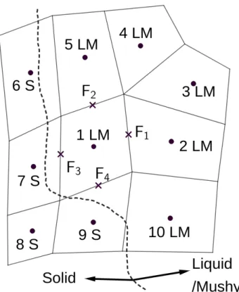
Figure 2.2 shows a typical distribution of phases during the solidification process. For ease of visualization, a two dimensional schematic is shown and the same idea has been generalized to three dimensions. The dotted line shows a solid-mushy zone interface. The control volumes (cells) on the left of the line are solid and on the right are either liquid or in mushy zone. Cells are labeled with tags S:Solid, LM: Liquid or Mushy. The S or LM tag is assigned to each cell based on the temperature at the previous time step and the liquidus and solidus temperatures of the alloy.
Figure 2.2: Control Volumes with Solid Liquid Interface
2.5.1
Momentum equation
As described in section 2.3, the modified momentum equations (2.7) are solved to estimate the intermediate velocities (u*). After discretization, the Darcy drag coefficient (Kµ) is added to the diagonal term of the linear equations. In the pure liquid region, this coefficient is zero and thus, it does not have any effect. In the mushy zone, it is finite and non-zero and thus, it acts like a resistance to the flow. In the fully solidified region, it is a large number and thus, the u* tends to zero. From computational efficiency point of view, it is not necessary to solve for u* in the solidified cells since it is zero. Therefore, at each time step, before solving the linearized system of equations, the matrix rows corresponding to solidified cells are removed. As these solidified cells are connected to the neighboring mushy or liquid zone cells, the rows corresponding to the neighboring cells have to be modified in a consistent
manner. Consider the row corresponding to cell number 1 in fig. 2.2: [A1, A2, . . . , A10] [φ1, φ2, . . . , φ10] T = [S1, S2, . . . , S10] T (2.16)
where, φ is any component of u* = [u∗, v∗, w∗]. Originally, φ1 is connected to all the neighboring cells from 2 to 10. But since cells 6, 7, 8 and 9 are solidified and their velocity is zero, those rows and columns are deleted from equation (2.16). Thus, the reduced row becomes: [A1, A2, A3, A4, A5, A10] [φ1, φ2, φ3, φ4, φ5, φ10] T = [S1, S2, S3, S4, S5, S10] T (2.17)
2.5.2
Pressure Poisson Equation
Similar to the momentum equations, the matrix rows corresponding to solidified cells are deleted from the discrete pressure Poisson equation. But in this case, the rows of the neighboring liquid or mushy cells cannot be updated by just deleting the connections of the solid cells as Neumann boundary conditions have to be applied. For any solidified cell, incoming or outgoing flow through all of its faces should be made zero. This is achieved as follows. Each face is shared by exactly 2 cells (face owners). All the cells which share a common vertex with a face are known as its neighbors. The face centered gradient is computed using the values at all connected neighboring cells. For example, cell numbers 1 and 2 are the owners of face F1 whereas, cells 1, 2, 3, 4, 5, 9 and 10 are its neighbors. The following cases arise for each face:
1. None of the neighbor cells is solidified: no change in the face centered gradient coeffi-cient is required (eg. all the faces of cell number 3)
2. None of the owners are solidified but at least one neighbor cell is solidified: flow through the face is allowed but the face centered gradient coefficient has to be modified as the
solidified cells are removed from the linear set of equation (eg. faces F1 and F2) 3. At least one owner is solidified: flow through the face is blocked; ∇P ·nˆ = 0 thus,
contribution of this face in the integrated diffusion term (‚SΓˆn· ∇P dS of eq. (2.12)) is zero (eg. faces F3 and F4)
Consider the face F2 for modification of face centered gradient coefficient. Original coeffi-cients for gradient computation at face F2 which are valid if none of its neighbor cells are solid are given by:
∂P ∂x ∂P ∂y F2 ≈ Ax1 Ax2 Ax3 Ax4 Ax5 Ax6 Ax7 Ay1 Ay2 Ay3 Ay4 Ay5 Ay6 Ay7 P 1 P2 P3 P4 P5 P6 P7 T (2.18) Since cell numbers 6 and 7 have solidified, their contribution has to be removed from equation (2.18). Thus, the last 2 columns are deleted and those coefficients are smeared equally in the remaining columns for ex., Ax1 is modified to Bx1 = Ax1 + (Ax6 +Ax7)/5 and Ay1 to
By1 =Ay1+ (Ay6+Ay7)/5. Since there are 5 cells remaining, the division by 5 is required. After modification, equation (2.18) becomes:
∂P ∂x ∂P ∂y F2 ≈ Bx1 Bx2 Bx3 Bx4 Bx5 By1 By2 By3 By4 By5 P1 P2 P3 P4 P5 T (2.19)
The steps for modification of the discretized pressure Poisson equation are as follows: 1. Identify the faces with none of the owners solidified but at least one neighbor cell is
3. Loop over all the cells:
If none of its face coefficients are modified, its coefficients do not change If at least one of its face coefficients is modified, re-assemble its coefficients These steps remove the contribution of the solidified cells carefully and reduce the compu-tational effort significantly.
2.5.3
Face Volume Flux Computation and Velocity Correction
The collocated finite volume formulation uses the face centered volume fluxes (ˆn·u∆A) in the continuity equation so as to avoid the checker-boarding of pressure. Thus, the volume flux passing through all the faces of a cell satisfies the discrete continuity equation i.e., the total volume flux entering a cell has to be balanced by the total volume flux exiting it to a specified tolerance level. If there is an inconsistency in the numerical formulation of the pressure Poisson equation and the flux computations, there can be a gain or loss of mass and convergence problems. This section describes a consistent method used in the current code to handle solidification.The volume flux is obtained by taking inner product of the velocity correction equation (2.9) at the face center with face normal and multiplying by face area:
ˆ n·un+1∆A f = ˆn·u*∆A f −nˆ·(∇P) n+1 ∆A f ∆t ρ (2.20) u* f
is estimated by averaging the cell values from the two owner cells of the face. ˆn · (∇P)n+1
f
is computed exactly in the same way as the regular diffusion term by splitting it into direct diffusion and cross diffusion terms (eq. (2.14) with φ =P). The face centered pressure gradient required in the cross diffusion term is estimated by the modified coefficients (eq. (2.19)). This volume flux estimate satisfying the discrete continuity equation to a specified tolerance is used in the convection term (eq. (2.7)). The cell centered velocities do
not satisfy the discrete continuity equation. They are computed from equation (2.9) and cell centered pressure gradient is estimated by averaging the face centered gradients.
2.5.4
Latent Heat Term
The Gulliver-Scheil equation (2.6) which relates temperature with solid fraction is a non-linear model. The easiest way to numerically couple this with the energy equation is to model the Gulliver-Scheil equation fully explicitly as a source term. The problem with an explicit approach is that the source term destabilizes the discretized energy equation due to high magnitude of the latent heat coefficient. Thus, we use the source term linearization concept discussed by Patankar [54]. The nonlinear term is split into a linear term and a remainder. The linear term is modeled implicitly and the remainder term is treated explicitly. From numerical stability point of view, the coefficient of the linear term which is added to the diagonal of the matrix should be positive. If the coefficient and the remainder term are functions of the unknown (temperature in this case), the equation has to be solved iteratively till convergence.
The latent heat term of the energy equation (2.4) when integrated over time and control volume gives: ˆ V ˆ t Lf ∂fs ∂t dV dt≈Lf∆V f m+1 s −f old s (2.21) where, superscriptsoldandm denote last time-step value and iteration number respectively. The value of solid fraction in the subsequent iteration (fm+1
s ) can be estimated from its latest value (fm
s ) by a first order Taylor expansion:
fsm+1 ≈fsm+ dfs dT m Tpm+1−Tpm (2.22)
Substituting equation (2.22) in (2.21) gives: ˆ V ˆ t Lf ∂fs ∂tdV dt≈Lf∆V fsm+ dfs dT m Tpm+1−Tpm−fsold = Lf∆V dfs dT m Tpm+1+ Lf∆V fsm−fsold− dfs dT m Tpm =SpTpm+1+Sc (2.23)
Sp and Sc are functions of last iteration and last time-step values and thus can be computed first. Note that Sp is always negative and when taken to the left hand side of the equation, it becomes positive and is thus added to the diagonal of the linear system matrix. Adding a positive term to the diagonal helps in stabilizing the system and speeds up convergence. Hence, this approach is found to be much better than the fully explicit method.
The Gulliver-Scheil equation (2.6) plotted in fig. 2.3afor a typical aluminum alloy shows that there is a discontinuity at the solidus temperature. Thus, the derivative dfsdT cannot be computed. To deal with this difficulty, the original equation is modified by smearing the discontinuity near the solidus temperature:
fs(T) = 0 if T > Tliq 1 if T < Tsol−T ˆ fs−(T −Tsol−T) 1−fsˆ 2T if Tsol−T < T < Tsol+T 1−TliqT−Tf−Tf 1 kp−1 otherwise (2.24) where, ˆfs = 1− Tsol+T−Tf Tliq−Tf kp1−1
and T is the width of linear smear which can be set to a reasonable value like 2 K. Thus, the derivative can be computed analytically. Figures 2.3b and 2.3c plot the modified solid fraction relation and its derivative respectively.
(a) Solid Fraction (b) Smeared Solid Fraction
(c) Derivative of Smeared Solid Fraction
Figure 2.3: Solid Fraction Temperature Relation
The overall iterative procedure to obtain the variables at the new time step from values at the old time step can be summarized as:
1. Initialize: T0
p =Tpold and fs0 =fsold
2. Compute Sp and Sc using last iteration values (Tpm and fsm) by equation (2.23) and solve the linear system of equations to estimate next iteration value Tm+1
p
3. Update the solid fraction: fsm+1 = (1−λ)fsm +λfs(Tpm+1) where, 0 < λ ≤ 1 is an under relaxation parameter (Note that fs(Tpm+1) is the solid fraction evaluated as a function of temperature at iterationm+ 1)
4. Estimate the relative change between the successive iteration values of temperature and solid fraction
Repeat steps 2 − 4 until the relative change drops below a desired threshold. For the aluminum alloy used here, it is found that under relaxation is not required i.e., λ = 1 and the solution converges in 5−10 iterations.
2.6
Solver for Linear Systems
Typical die cast geometries have high aspect ratios i.e., thin cross sections compared to the lateral dimensions. It is found that single grid iterative solvers for the elliptic pressure Poisson equation converge slowly for such geometries. Hence, in this work a multigrid solver is used. The central idea of a multigrid solver is to solve the equations on multiple coarse grids and couple the corrections from all the grids through prolongation and relaxation. The high frequency component of the residual converges fast on the fine grids while the coarse grids are used to accelerate convergence of the low frequency residual. Thus, the coarse grid solutions are used to accelerate the convergence while maintaining the discretization accuracy of the solution at the finest level.
Geometric multigrid is a technique in which multiple levels of grids are generated phys-ically and the matrix vector system is estimated by discretizing the governing equations at each level. The main benefit of this approach is that the matrices at all the levels are obtained directly from the governing equations and thus, good convergence is observed. The main drawback is that generating coarse grids for a complex geometry with unstructured elements is non-trivial. Algebraic multigrid (AMG) tries to address this problem by coars-ening the matrix using heuristics based algorithms. This is a black box approach which does not need any physical grids at coarse levels.
The BoomerAMG routine along with Krylov solvers of the open source library HYPRE [39] developed at the Lawrence Livermore National Laboratory is used in our work. The AMG solver is observed to solve the modified momentum equations (2.7) and the energy equation (2.4) without difficulty. However, some consistency issues have been observed
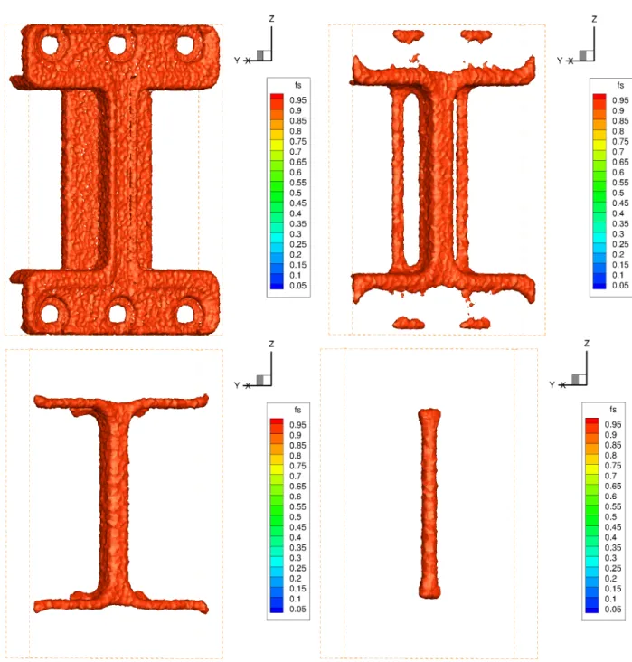
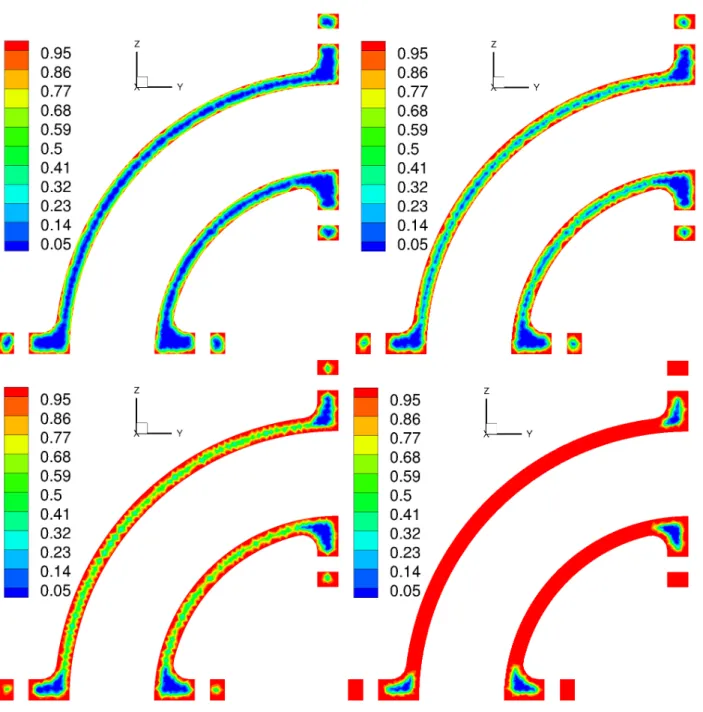
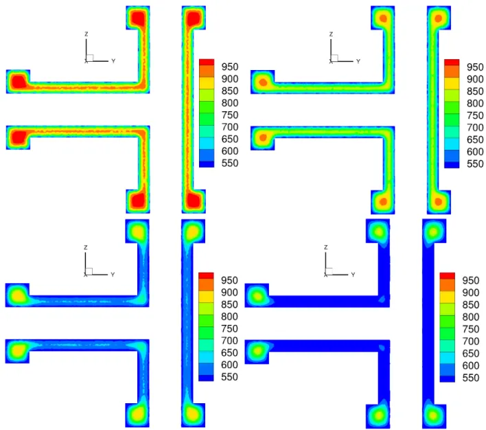
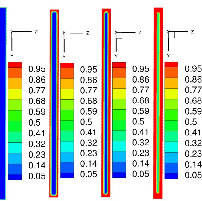
during the solution of the pressure Poisson equation (2.10) when extensive solidification happens. In complex geometries, as solidification proceeds, there can be disjoint pockets of metal which are yet to solidify. Figure 2.4 shows an example of the disjoint regions formed near the end of solidification. The area with solid fraction of unity (red in fig. 2.4b) is fully solidified and thus, has zero velocity and the pressure is also set to zero. The blue regions indicate liquid/mushy zones which are yet to solidify. These regions are solved with zero normal velocities on their boundaries. Each region is solved with Neumann pressure boundary conditions corresponding to fixed velocities on the boundary. We have checked that the sums of the local sources/sinks of the pressure Poisson equation for individual regions are zero. Thus, the pressure Poisson equation is well formulated whether solved separately for each domain or as a single linear system. As these pockets are far enough from each other, they are decoupled numerically in the discrete reduced pressure Poisson equation (section 2.5.2). This is seen to cause convergence difficulties with AMG. The AMG solver has been coupled with a single grid BiCGSTAB solver, also from HYPRE, to be used when AMG is unable to solve the pressure Poisson equation. This issue arises towards the end of the simulation when only a few cells are liquid (for instance 20%). Thus, the reduced system is much smaller in size compared to the original problem and a single grid solver is reasonably well convergent.
(a) Temperature (K) (b) Solid Fraction
(c) Pressure (Pa)
Figure 2.4: Disjoint Regions near the End of Solidification
2.7
Grain Growth and Mechanical Properties Models
Grain size and Secondary Dendrite Arm Spacing (SDAS) are two important parameters used to characterize the microstructure. OpenCast uses empirical relations from the literature for estimation of microstructure parameters and mechanical properties such as yield strength.
SDAS is predicted based on the empirical relationship discussed by Backer and Wang [22], SDAS =λ2 =Aλ ∂T ∂t Bλ [in µm]. (2.25)
The model parameters Aλ and Bλ are chosen to be 39.4 and -0.317, respectively based on the model for microstructure in aluminum alloys [22]. Material behavior of the die cast alloy is predicted in terms of 2% yield strength (σ0.2) using empirical relationship proposed by Okayasu et al. [58].
σ0.2 =Aσλ −1/2
2 +Bσ (2.26)
Here, σ0.2 is in MPa, λ2 (SDAS) is in µm,Aσ = 59.0 and Bσ = 120.3 [58].
Grain size estimation is based on the work of Greer et al. [24]. The grain growth rate is given by: dr dt = λ2 sDs 2r (2.27)
where,r is the grain size,Ds is the solute diffusion coefficient in the liquid andtis the time. The parameter λs is obtained by invariant size approximation:
λs= −S 2π0.5 + S2 4π −S 0.5 (2.28) S is given by S = 2(Cs−C0) Cs−Cl (2.29) where, Cl = C0(1−fs)(kp−1) is solute content in the liquid, Cs = kpCl is solute content in the solid at the solid-liquid interface and C0 is the nominal solute concentration. Thus, using the prescribed partition coefficient (kp) and estimated solid fraction (fs), equations (2.27)–(2.29) are solved to get the final grain size.
Chapter 3
Parameter Uncertainty Quantification
3.1
Introduction
Final product quality in die casting is influenced by many process parameters like alloy ma-terial properties, interface conditions at the mold, thermal boundary conditions etc. Mea-suring and controlling these parameters accurately is difficult due to the complexity of the process. This stochastic variation is dealt as parameter uncertainty in the numerical simula-tions. Conventional deterministic simulations alone are unable to estimate its effect on the product quality. From modeling perspective, parameter uncertainty quantification is a set of partial differential equations with coefficients, boundary conditions or initial conditions varying stochastically. The basic idea is to consider the stochastic variables as dimensions of the problem in addition to space and time.
In the recent years, there has been a growing interest in analysis of the effects of stochas-tic variations in the inputs on the outputs. There are multiple examples in the literature in which the uncertainty propagation techniques are combined with the deterministic numerical simulations [26–35, 59, 60]. It is popular to use the polynomial chaos expansion (PCE) for uncertainty propagation in which the output is approximated as a summation of polynomial basis which are functions of the stochastic inputs. Two main classes of methods to estimate the coefficients of the PCE are stochastic Galerkin projection [26–28, 59] and collocation [29–31]. Stochastic Galerkin method is intrusive since it requires solution of a new set of equations and thus, the underlying deterministic code has to be modified. This becomes a significant additional effort of software development and difficult to couple with the legacy
codes. Hence, recently non-intrusive stochastic collocation methods have been gained pop-ularity. The basic idea is to have multiple evaluations of the deterministic simulation at predefined collocation points which are samples from the underlying probability distribution function of the input parameters. The PCE coefficients are then estimated from the output values obtained from the deterministic solution at these input samples. The coefficients can be used for post-processing operations like output statistics estimation, response surface plotting and sensitivity analysis.
The PCE method is extremely useful for low dimensional uncertainty quantification. But at higher dimensions, it faces a problem known as ‘curse of dimensionality’ i.e., for a linear increase in the stochastic dimensions, the number of samples grows exponentially. The Smolyak algorithm [61] addresses this problem to some extent by reducing the number of samples in high dimensional stochastic space without compromising the interpolation accuracy. Even with the use of Smolyak algorithm, number of samples required is of the order of 103 −104 for five or more input dimensions. For instance, an eight and sixteen dimensional problem needs 3905 and 51073 samples respectively, for an accuracy level of five [62]. Practically, it is computationally expensive to simulate the deterministic software thousands of times. Thus, an alternate method is required for uncertainty propagation.
The Monte Carlo is a simple method which approximates the statistics of the output by running the deterministic simulations at pseudo random samples of the inputs [63]. Let
w(x,ξ) be a function which maps inputs to an output. Here, the vector x denotes all the deterministic inputs whereas, the vector ξ denotes all the stochastic parameters. It is assumed that the stochastic variable follows a known probability distribution: ξ ∼ f(ξ). The aim is to estimate the stochastic mean of the output w(x,ξ) defined as:
wf(x) =
ˆ
w(x,ξ)f(ξ)dξ (3.1)
approx-imated numerically. Importance sampling based Monte Carlo approximation of the integral is given by [63]: wf(x)≈ 1 n i=n X i=1 w(x,ξi) f(ξi) p(ξi) (3.2)
where, ξi are n samples drawn from the probability distribution p(ξ). It is effective to set
p(ξ) as f(ξ) to reduce variance i.e.,ξi ∼f(ξ) [63]. Thus, eq. (3.2) is simplified to:
wf(x)≈ 1 n i=n X i=1 w(x,ξi) (3.3)
Since the error using the Monte Carlo method is O(1/√n), the number of samples is practically too high which makes using the Monte Carlo method directly with the determin-istic simulation difficult. Thus, it is popular to use a surrogate model which is trained and tested using deterministic simulations. A good surrogate model can be trained with small number of deterministic simulations and its evaluation is cheap. A well tested surrogate model is further used to estimate the outputs at multiple sample inputs. Since the surrogate model evaluation is cheap, there is practically no limit on the number of input samples for Monte Carlo method. Note that the PCE is also a surrogate model which is ideal for lower stochastic dimensions with a possibility of direct estimation of the output statistics without the use of Monte Carlo method. Thus, in this research, PCE and neural network are used as surrogates for low and high dimensional stochastic problems respectively. This chapter summarizes the theory for both of them.
3.2
Polynomial Chaos Expansion
To estimate the relation between stochastic process parameters and output parameters, var-ious methods have been proposed in the literature. A popular method is to use a linear combination of polynomial basis functions in the stochastic dimension to expand the output variables. Since orthogonality helps in convergence, orthogonal polynomials are used as basis
functions. Wiener’s polynomial chaos [64] with Askey family of orthogonal polynomials leads to optimal convergence of the error. Xiu and Karniadakis [65] determined which polyno-mial leads to exponential convergence depending on the underlying probability distribution function that the stochastic variable follows. For instance, the Hermite polynomials are or-thogonal with respect to the standard normal distribution as the weighting function. Hence, it is recommended to use Hermite polynomials as basis functions if the stochastic variable follows normal distribution. Using generalized polynomial chaos expansion developed by Xiu and Karniadakis [65], a second order random field (w) can be expanded by polynomial basis (eq. (3.4)). For all practical purposes, the series is truncated to order n.
w(x,ξ(θ)) = ∞ X i=0 wi(x)Ψi(ξ(θ))≈ n X i=0 wi(x)Ψi(ξ(θ)) (3.4) where, w is the quantity of interest, x is a vector of all the deterministic inputs including space and time (if applicable), Ψi is the multi-dimensional orthogonal polynomial of order
i, ξ is the random variable vector (ξ1, ξ2, . . . ξn) and θ is an elementary event.
In this work, stochastic collocation method is used to estimate the deterministic coeffi-cients of the polynomial chaos expansion. Collocation is a non-intrusive method and thus, modification of deterministic software is not necessary. It acts as a wrapper around existing deterministic software. The deterministic simulation is run at M sample points (ξm) and a condition w(x,ξm) = w
sim(x,ξm) is imposed. The right hand side comes from each deter-ministic simulation and left hand side from polynomial expansion. This givesM constraints written in a matrix vector form [66]. M > n + 1 ensures that the Vandermonde system
(eq. (3.5)) is overdetermined. Solving in the least-squares sense gives w0(x) · · · wn(x) T . Ψ0(ξ1) · · · Ψn(ξ1) .. . ... Ψ0 ξM · · · Ψn ξM w0(x) .. . wn(x) = wsim(x,ξ1) .. . wsim x,ξM (3.5)
Sample points (ξm) have to be chosen wisely for successive implementation of stochastic collocation method. For instance, uniformly distributed samples can lead to highly oscil-latory basis functions and thus poor convergence. Thus, for one dimensional stochastic problems [66], it is popular to choose roots of the basis orthogonal polynomial as sample points. For multiple stochastic dimensions, a simple idea is to use a tensor product of sin-gle dimensional samples. The problem with tensor products is that the number of samples grows exponentially with stochastic dimensions. Each sample corresponds to a deterministic simulation and thus, the computational expense grows exponentially. Smolyak [61] came up with an algorithm to reduce number of samples in multi-dimensional space maintaining the accuracy of the interpolation. In this research, sparse grid nodes are taken from the work of Heiss and Winschel [62]. A MATLAB based tool UQLab developed by Marelli and Sudret [67] is used for post processing the simulation outputs to estimate polynomial chaos coefficients and generate the response surfaces.
The strategy described above is quite general and can be applied to any numerical solution framework. For instance in the current work, the output variables (w of eq. (3.4)) could be temperature and microstructure parameters like grain size and dendritic arm spacing. The stochastic input parameters could be boundary conditions, initial conditions and alloy and material properties. The polynomial chaos expansion with stochastic collocation is combined
with the deterministic computational fluid flow and heat transfer solver to estimate the sensitivity and uncertainty propagation.
3.3
Deep Neural Network
A neural network is a set of interconnected nodes such that the information flows from inputs to outputs. Each node is known as a neuron. Figure3.1a shows a single neuron which has n scalar inputs (x1, x2, ..., xn) and single output (y). Each neuron performs the following two operations in sequence:
1. Linear transformation: a = Pni=1wixi +b; where, wi are the weights and b is a bias term
2. Element-wise nonlinear transformation: y=σ(a); where, σ is the activation function A neural network is formed by stacking single neurons in a layer and connecting multiple layers as shown in fig. 3.1b. It depicts an input (layer L1), an output (layer L4) and two hidden layers (layers L2 and L3). The arrows indicate the direction of information flow from input to output layer through the hidden layers. A deep neural network (DNN) is essentially a neural network with multiple hidden layers. Adding multiple hidden layers increases the nonlinearity of the network and thus, the network can approximate more complex functions successfully. The number of neurons in the input and output layers is specified by the problem definition whereas, number of hidden layers and neurons has to be fine tuned.
(a) Single Neuron (b) Deep Neural Network
Figure 3.1: Neural Network Schematics
The linear transformation followed by the nonlinear activation function of each neuron can be written in a single matrix vector equation:
y(j) = x if j = 1 σ(W(j)y(j−1)+b(j)) ∀j ∈ {2,3, ..., L} (3.6)
where, the input vector x ∈ Rl1, weights W(j) ∈
Rlj×lj−1, activation produced by the jth
layer y(j) ∈
Rlj and bias b(j) ∈ Rlj. L is the total number of layers including input, output
and hidden layers. Number of neurons in the jth layer is denoted by l
j. For instance, in figure 3.1b, L = 4, l1 = 4, l4 = 8 and l2 = l3 = 6. Applying equation (3.6) sequentially starting from the input layer is known as forward propagation. This operation estimates the output vector (y(L)) from the input vector (y(1) = x) for given values of weights and bias. Logistic sigmoid, hyperbolic tangent and rectified linear unit (ReLU) are some of the popular