Electrical and Computer Engineering Publications
Electrical and Computer Engineering
2016
Work-Efficient Parallel and Incremental Graph
Connectivity
Natcha Simsiri
University of Massachusetts-Amherst
Kanat Tangwongsan
Mahidol University International College
Srikanta Tirthapura
Iowa State University, [email protected]
IBM T.J. Watson Research Center
Follow this and additional works at:
https://lib.dr.iastate.edu/ece_pubs
Part of the
Computer Sciences Commons, and the
Electrical and Computer Engineering
Commons
The complete bibliographic information for this item can be found at
https://lib.dr.iastate.edu/
ece_pubs/170. For information on how to cite this item, please visit
http://lib.dr.iastate.edu/
howtocite.html.
This Article is brought to you for free and open access by the Electrical and Computer Engineering at Iowa State University Digital Repository. It has been accepted for inclusion in Electrical and Computer Engineering Publications by an authorized administrator of Iowa State University Digital Repository. For more information, please [email protected].
Work-Efficient Parallel and Incremental Graph Connectivity
AbstractOn an evolving graph that is continuously updated by a high-velocity stream of edges, how can one efficiently maintain if two vertices are connected? This is the connectivity problem, a fundamental and widely studied problem on graphs. We present the first shared-memory parallel algorithm for incremental graph connectivity that is both provably work-efficient and has polylogarithmic parallel depth. We also present a simpler
algorithm with slightly worse theoretical properties, but which is easier to implement and has good practical performance. Our experiments show a throughput of hundreds of millions of edges per second on a 20-core machine.
Disciplines
Computer Sciences | Electrical and Computer Engineering
Comments
This is a manuscript of the article Simsiri, Natcha, Kanat Tangwongsan, Srikanta Tirthapura, and Kun-Lung Wu. "Work-efficient parallel and incremental graph connectivity."arXiv preprint arXiv:1602.05232(2016). Posted with permission.
Work-E
ffi
cient Parallel and Incremental Graph Connectivity
Natcha Simsiri˚ Kanat Tangwongsan: Srikanta Tirthapura; Kun-Lung Wu§February 18, 2016
Abstract
On an evolving graph that is continuously updated by a high-velocity stream of edges, how can one
efficiently maintain if two vertices are connected? This is the connectivity problem, a fundamental and
widely studied problem on graphs. We present the first shared-memory parallel algorithm for incremental
graph connectivity that is both provably work-efficient and has polylogarithmic parallel depth. We also
present a simpler algorithm with slightly worse theoretical properties, but which is easier to implement and has good practical performance. Our experiments show a throughput of hundreds of millions of edges per second on a 20-core machine.
1
Introduction
Graph connectivity is a fundamental problem with a long history. On an undirected graph, the basic connectivity question is:given two vertices, is there a path between them?
Our work is motivated by the need for high throughput real-time streaming graph analytics. Every minute, a staggering amount of high-velocity linked data is being generated from social media interactions, the Internet of Things (IoT) devices, among others—and timely insights from them are much sought after. These data are usually cast as a stream of edges with the goal of maintaining certain local and global properties on the accumulated data. Modern stream processing systems such as IBM Infosphere Streams [10] and Apache Spark [19] rely on parallel processing of input streams to achieve high throughput and real-time analytics. However, these systems only provide the software infrastructure; scalable, parallel, and dynamic graph algorithms are still needed to make use of the potential of these systems.
As a first step towards efficient parallel and dynamic graph algorithms, we consider the parallel incre-mentalgraph connectivity problem in a setting where edges and queries arrive in bulk. Tackling the parallel incremental version of the problem, which allows only addition of edges to the graph, is an important stepping stone towards the more general problem of (fully)dynamicconnectivity that allows both addition and deletion of edges.
There exist sequential algorithms for incremental graph connectivity, starting from the popular union-find data structure [18]; but these are, for the most part, unable to take advantage of parallelism. There exist parallel algorithms for graph connectivity (e.g., [17, 9]), but these are, for the most part, not incremental. None of these meet the need for high throughput dynamic graph processing.
˚College of Information and Computer Sciences, University of Massachusetts-Amherst,[email protected] :Computer Science Program, Mahidol University International College,[email protected]
;Department of Electrical and Computer Engineering, Iowa State University,[email protected] §
IBM T.J. Watson Research [email protected]
In order to make effective use of parallelism in stream processing, systems such as Apache Spark [19] use a model of “discretized streams”, where the incoming high-volume stream is divided into a sequence of “minibatches”. Each minibatch is processed using a parallel computation, and the resulting system can potentially achieve a very high throughput, subject to the availability of appropriate algorithms. We adopt this model in our work and seek parallel methods that can process a minibatch of edges efficiently.
Model:On a vertex setV, a graph streamAis a sequence of minibatchesA1,A2, . . ., where each minibatch
Aiis a set of edges onV. The graph at the end of observingAt, denoted byGt, isGt “ pV,Yti“1Aiqcontaining all the edges up tot. The minibatchesAineed not be of equal sizes.
In this paper, we study abulk-parallel incremental connectivity problem, which is to maintain a data structure that provides two operations:Bulk-UpdateandBulk-Query. TheBulk-Updateoperation takes as input a minibatch of edgesAiand adds them to the graph. TheBulk-Queryoperation takes a minibatch of vertex-pair queries and returns for each query, whether the two vertices are connected on the edges observed so far in the stream. On this data structure, theBulk-QueryandBulk-Updateoperations are each invoked with a (potentially large) minibatch of input, each processed using a parallel computation. But a bulk operation, say aBulk-Update, must complete before the next operation, say aBulk-Query, can begin.
Contributions: We present the first shared-memory parallel algorithm for incremental connectivity that
is both provably work-efficient and has polylogarithmic parallel depth. We make the following specific contributions:
— Simple Parallel Incremental Connectivity.We first present a simple algorithm that is easy to implement, yet has good theoretical properties. On a graph withnvertices, this algorithm makes a single pass through the stream usingOpnqmemory, and can process a minibatch ofbedges, usingOpblognqwork andOppolylogpnqq parallel depth. We describe this algorithm in Section 4.
— Work-Efficient Parallel Incremental Connectivity.We present an improved parallel algorithm with total workOppm`qqαpm`q,nqqwheremis the total number of edges across all minibatches,qis the total number of connectivity queries across all minibatches, andαis an inverse Ackermann’s function (see Section 2). This matches the work of the best sequential counterpart, which makes this parallel algorithmwork-efficient. Further, the parallel depth of processing a minibatch is polylogarithmic. Hence, the sequential bottleneck in the runtime of the parallel algorithm is very small, and the algorithm is capable of using almost a linear number of processors efficiently. We are not aware of a prior parallel algorithm with such provable properties on work and depth. We describe this algorithm in Section 5.
— Implementation and Evaluation.We implemented and benchmarked a variation of our simple parallel algorithm on a shared-memory machine. Our experimental results show that the algorithm achieves good speedups in practice and is able to efficiently use the available parallelism. On a 20-core machine, it can process hundreds of millions of edges per second, and realize a speedup of 8–11x over its single threaded performance. Further analysis shows good scalability properties as the number of threads is varied. We describe this in Section 6.
2
Related Work
Letnbe the number of vertices,mthe number of operations, andαan inverse Ackermann’s function (very slow-growing, practically a constant independent ofn). In the sequential setting, the basic data structure for incremental connectivity is the well-studied union-find data structure [5]. Tarjan [18] achieves anOpαpm,nqq amortized time perfind, which has been shown to be optimal (see Seidel and Sharir [15] for an alternate analysis).
Recent work on streaming graph algorithms focuses on minimizing the memory requirement, with little attention given to the use of parallelism. This line of work has largely focused on the “semi-streaming model” [8], which allowsOpn¨polylogpnqqspace usage. In this model, the union-find data structure [18] solves incremental connectivity inOpnqspace and a total time nearly linear inm.
When only opnq of workspace (sublinear) is allowed, interesting tradeoffs are known for multi-pass algorithms. For an allotment of Opsq workspace, an algorithm needsΩpn{sq passes [8] to compute the connected components of a graph. Demetrescu et al. [7] consider the W-stream model, which allows the processing of streams in multiple passes in a pipelined manner: the output of thei-th pass is given as input to thepi`1q-th pass. They show a tradeoffbetween the number of passes and the memory required. Withsbits of space, their algorithm computes connected components inOppnlognq{sqpasses. Demetrescu et al. [6] present a simulation of a PRAM algorithm on the W-Stream model, allowing existing PRAM algorithms to runsequentiallyin the W-Stream model.
McColl et al. [13] present a parallel algorithm for maintaining connected components in a fully dy-namic graph, which handles edge deletions—a more general setting than ours. As part of a bigger project (STINGER), their work focuses on engineering algorithms that work well on real-world graphs and gives no theoretical analysis of the parallel complexity. In contrast, this work focuses on achieving the best theoretical efficiency, matching the work of the best sequential counterpart.
Berry et al. [2] present methods for maintaining connected components in their parallel graph stream model, called X-Stream, which periodically ages out edges. Their algorithm is essentially an “unrolling” of the algorithm of [7], and edges are passed from one processor to another until the connected components are found by the last processor in the sequence. Compared to our work, the input model and notions of correctness differ. Our work views the input stream a sequence of batches, each a set of edges or a set of queries, which are unordered within the set. Their algorithm strictly respects the sequential ordering the edges and queries. Further, they age out edges (we do not). Also, they do not give provable parallel complexity bounds.
There are multiple parallel (batch) algorithms for graph connectivity including [17, 9] that are work-efficient (linear in the number of edges) and that have polylogarithmic depth. Prior work on wait-free implementations of the union-find data structure [1] focuses on the asynchronous model, where the goal is to be correct under all possible interleavings of operations; unlike us, they do not focus on bulk processing of edges. There is also a long line of work on sequential algorithms for maintaining graph connectivity on an evolving graph. See the recent work by [12] that addresses this problem in the general dynamic case and the references therein.
3
Preliminaries and Notation
Throughout the paper, letrnsdenote the sett0,1, . . . ,nu. A sequence is written asX “ xx1,x2, . . . ,x|X|y, where|X|denotes the length of the sequence. For a sequenceX, thei-th element is denoted byXi orXris. Following the set-builder notation, we denote byxfpxq : Φpxqya sequence generated (logically) by taking all elements that satisfyΦpxq, preserving their original ordering, and transform them by applying f. For example, if T is a sequence of numbers, the notationx1` fpxq : x P T andxoddymeans a sequence created by taking each elementxfromT that are odd and mapxto 1`fpxq, retaining their original ordering. Furthermore, we writeS ‘T to mean the concatenation ofS andT.
We design algorithms in the work-depth model assuming an underlying CRCW PRAM machine model. As is standard, theworkof an algorithm is the total operation count, and thedepth(also called parallel time or span) is the length of the longest chain of dependencies within a parallel computation. The gold standard
for algorithms in this model is to perform the same amount of work as the best sequential counterpart (work efficient) and to have polylogarithmic depth. We remark that an algorithm designed for the CRCW model can work in other shared memory models such as EREW PRAM, with a depth that is a logarithmic factor worse. We use standard parallel operations such as filter, prefix sum, map (applying a constant-cost function), and pack, all of which hasOpnqwork and at mostOplog2pnqqdepth on an input sequence of lengthn. Given a sequence ofmnumbers, there is a duplicate removal algorithmremoveDuprunning inOpmqwork and
Oplog2mqdepth [11]. We also use the following results to sort integer keys in a small range faster than a typical comparison-based algorithm:
Theorem 1 (Parallel Integer Sort [14]) There is an algorithmintSortthat takes a sequence of integer
keys a1,a2, . . . ,an, each a number between0and c¨n, where c“Op1q, and produces a sorted sequence in
Opnqwork andpolylogpnqdepth.
Parallel Connectivity:For a graphG“ pV,Eq, a connected component algorithm (CC) computes a sequence
of connected components ofG xCiyki“1, where eachCi is a list of vertices in the component. There are algorithms forCCthat haveOp|V| ` |E|qwork andOppolylogp|V|,|E|qqdepth (e.g., [9, 17]), with Gazit’s algorithm [9] requiringOplog|V|qdepth.
4
Simple Bulk-Parallel Data Structure
This section describes a simple bulk-parallel data structure for incremental graph connectivity. We describe theoretical improvements to this basic version in the next section. As before,nis the number of vertices in the graph stream. The main result for this section is as follows:
Theorem 2 There is a bulk-parallel data structure for incremental connectivity, given by Algorithms
Simple-Bulk-QueryandSimple-Bulk-Update, where
(1) The total memory consumption is Opnqwords.
(2) A minibatch of b edges is processed bySimple-Bulk-Updatein Oplogpmintb,nuqqparallel depth and Opblognqtotal work.
(3) A minibatch of q connectivity queries, each asking for connectivity between two vertices, is answered
bySimple-Bulk-Queryin Oplognqparallel depth and Opqlognqtotal work.
In a nutshell, we show how to bootstrap a standard union-find structure to take advantage of parallelism while preserving the height of the union-find forest to be at mostOplognq. For concreteness, we will work with union by size, though other variants (e.g., union by rank) will also work.
Union-Find: We review a basic union-find implementation that uses union by size. From the viewpoint
of graph connectivity, union-find maintains connectivity information about a graph with verticesV “ rns supporting:
• foruPV,findpuq PVreturns an identifier of the connected component thatubelongs to. This has the property thatfindpuq “findpvqif and only ifuandvare connected in the graph.
• foru,vPV,unionpu,vqlinksuandvtogether, making them in the same connected component. It also
returns the identifier of the component that bothuandvnow belong to—this is the same identifier one would get from runningfindpuqorfindpvqat this point.
Conceptually, this data structure maintains a union-find forest, one tree for each connected component. In this view,findpuqreturns the vertex that is the root of the tree containinguandunionpu,vqjoins together
the roots of the tree containinguand the tree containingv. The trees in a union-find forest are typically represented by remembering each node’s parent, in an arrayparentof lengthn, whereparentrusis the tree’s parent ofuorparentrus “uif it is the root of its component.
The running time of the union and find operations depends on the maximum height of a tree in the union-find forest. To keep the height small, at mostOplognq, a simple strategy, known asunion by size, is for
unionto always link the tree with fewer vertices into the tree with more vertices. The data structure also
keeps an array for the sizes of the trees. The following results are standard (see [15], for example):
Lemma 3 (Sequential Union-Find) On a graph with verticesrns, a sequential union-find data structure
implementing the union-by-size strategy consumes Opnqspace and has the following characteristics: • Every union-find tree has height Oplognqand eachfindtakes Oplognqsequential time.
• Given two distinct roots u and v, the operation unionpu,vq implementing union by size takes Op1q
sequential time.
Our data structure maintains an instance of this union-find data structure, calledU. Notice that thefind
operation is read-only. Unlike the more sophisticated variants, this version of union-find does not perform path compression.
4.1 Answering Connectivity Queries in Parallel
Connectivity queries can be easily answered in parallel, using read-onlyfinds onU. To answer whether
u and v are connected, we compute U.findpvq and U.findpuq, and report if the results are equal. To answer multiple queries in parallel, we note that because thefinds are read-only, we can answer all queries simultaneously independently of each other. We presentSimple-Bulk-Queryin Algorithm 1.
Algorithm 1:Simple-Bulk-QuerypU,xpui,viqy q i“1).
Input:Uis the union find structure, andpui,viqis a pair of vertices, fori“1, . . . ,q. Output: For eachi, whether or notuiis connected toviin the graph.
1: fori“1,2, . . . ,qdoin parallel 2: aiÐ pU.findpuiq ““U.findpviqq
3: returnxa1,a2, . . . ,aqy
Correctness follows directly from the correctness of the base union-find structure. The parallel complexity is simply that of applyingqoperations ofU.findin parallel:
Lemma 4 The parallel depth ofSimple-Bulk-Queryis Oplognq, and the work is Opqlognq, where q is
the number of queries input to the algorithm. 4.2 Adding a Minibatch of Edges
How can one incorporate (in parallel) a minibatch of edges A into an existing union-find structure? Sequen-tially, this is simple: invokeunionon the endpoints of every edge ofA. To make it parallel, though, we cannot blindly apply theunionoperations in parallel. Becauseunionupdates the forest, running multiple
unionoperations independently in parallel can create inconsistencies in the structure.
We observe, however, that it is safe run multipleunions in parallel as long as they operate on different trees. This is not sufficient, as there may be a number of union operations involving the same tree, and
running these sequentially will result in a large parallel depth. For instance, consider adding the edges of a star graph (with a very high degree) to an empty graph. Because all the edges share a common endpoint, the center of the star is involved in everyunion, and hence no two operations can proceed in parallel.
To tackle this problem, our algorithm transforms the minibatch of edges Ainto a structure that can be connected up easily in parallel. For illustration, we revisit the example when the minibatch is itself a star graph. Suppose there are seven edges within the minibatch: pv1,v2q,pv1,v3q,pv1,v4q, . . . ,pv1,v8q. By
examining the minibatch, we find that all ofv1, . . . ,v8will belong to the same component. We now apply these connections to the graph.
In terms of connectivity, it does not matter whether we apply the actual edges that arrived, or a different, but equivalent set of edges; it only matters that the relevant vertices are connected up. To connect up these vertices, our algorithm schedules theunions in only three parallel rounds as follows. The notationX}Y
indicates thatXandYare run in parallel:
1: unionpv1,v2q}unionpv3,v4q}unionpv5,v6q}unionpv7,v8q 2: unionpv1,v3q}unionpv5,v7q
3: unionpv1,v5q
As we will soon see, such a schedule can be constructed for a component of any size provided that no two of vertices in the component are connected previously. The resulting parallel depth is logarithmic in the size of the minibatch.
Algorithm 2:Simple-Bulk-UpdatepU,Aq
Input:U: the union find structure,A: a set of edges to add to the graph.
B Relabel eachpu,vqwith the roots ofuandv
1: A1Ð xppu,pvq : pu,vq PAwherepu “U.findpuqandpv“U.findpvqy B Remove self-loops 2: A2Ð xpu,vq : pu,vq PA1whereu ,vy 3: CÐCCpA2q 4: foreachCPCdoin parallel 5: Parallel-JoinpU,Cq
To add a minibatch of edges, ourSimple-Bulk-Updatealgorithm, presented in Algorithm 2, proceeds in three steps:
BStep 1: Relabel edges as links between existing components. An edgetu,vu P Adoes not simply join
verticesuandv. Due to potential existing connections inG, it joins togetherCu andCv, the component containing u and the component containing v, respectively. In our representation, the identifier of the component containinguisU.findpuq, soCu “ U.findpuqand similarlyCv “ U.findpvq. Lines 1-2 in Algorithm 2 create A2 by relabeling each endpoint of an edge with the identifier of its component, and
dropping edges that are within the same component.
BStep 2: Discover new connections arising fromA. After the relabeling step, we are implicitly working with
the graph ˜H“ pVH˜,A2q, whereVH˜ is the set of all connected components ofGthat pertain toA(i.e., all the
roots in the union-find forest reachable from vertices incident onA) andA2is the connections between them. In other words, ˜His a graph on “supernodes” and the connections between them using the edges ofA. In this view, a connected component on ˜Hrepresents a group of existing components ofGthat have just become connected as a result of incorporatingA. While never materializing the vertex setVH˜, Line 3 in Algorithm 2
computesC, the set of connected components of ˜H, using a linear-work parallel algorithm for connected components,CC(see Section 3).
BStep 3:Commit new connections toU. With the preparation done so far, the final step only has to make sure that the pieces of each connected component inCare linked together inU. Lines 4-5 of Algorithm 2 go over the components ofCin parallel, seeking help fromParallel-Join, the real workhorse that links together the pieces.
Connecting a Set of Components withinU: Letv1,v2, . . . ,vk P rnsbe distinct tree roots from the union-find forestUthat form a component inC, and need to be connected together. AlgorithmParallel-Join
connects them up inOplogkqiterations using a divide-and-conquer approach. Given a sequence of tree roots, the algorithm splits the sequence in half and recursively connects the roots in the first half, in parallel with connecting the roots in the second half. Since components in the first half and the second half have no common vertices, handling them in parallel will not cause a conflict. Once both calls return with their respective new roots, they are unioned together.
Algorithm 3:Parallel-JoinpU,Cq
Input:U: the union-find structure,C: a seq. of tree roots Output: The root of the tree after all ofCare connected 1: if|C| ““1then
2: returnCr1s
3: else
4: `Ðt|C|{2u
5: uÐParallel-JoinpU,Cr1,2, . . . , `sqin parallel with vÐParallel-JoinpU,Cr``1, ``2, . . . ,|C|sq
6: returnU.unionpu,vq
Correctness ofParallel-Joinis immediate since the order that the unioncalls are made does not matter, and we know that differentunioncalls that proceed in parallel always work on separate sets of tree roots, posing no conflicts.
Lemma 5 Given k distinct roots of U, AlgorithmParallel-Joinruns in Opkqwork and Oplogkqdepth.
Lemma 6 (Correctness ofSimple-Bulk-Update) If U is the shared-memory union-find data structure
formed by a sequence of minibatch arrivals whose union equals the graph G, then for any u,v P V, U.findpuq “U.findpvqif and only if u and v are connected in G.
Proof: Consider a minibatch of edgesA. LetG1be the set of edges that arrived prior toAandU1the state of the union-find structure formed by insertingG1. LetG2 “G1YAand letU2be the state of the union-find
structure afterSimple-Bulk-UpdatepU1,Aq. We will assume inductively thatU1is correct with respect to
G1and show thatU2is correct with respect toG2.
Letx,ybe a pair of vertices inV. We consider the following two cases.
Case I: x andy are not connected inG2. In this case, x andy are not connected inG1 either. Let
rx “U1.findpxq,ry “U1.findpyq. From the inductive assumption, we knowrx ,ry. Note thatAwill not contain a path betweenxandy. Hence inC, the connected components ofA2,rxandrywill not be in the same component. WhenCis applied toU1inParallel-Join, the components containingrx andry are not linked together, and hence it is still true thatU2.findpxq “U2.findprxq,U2.findpryq “U2.findpyq.
Case II: x andy are connected inG2. There must be a path x “ v1,v2, . . . ,vt “ y inG2. We will
show that U2.findpv1q “ U2.findpv2q “ . . . “ U2.findpvtq, leading to the conclusionU2.findpxq “
denote the roots of the trees that containviandvi`1respectively inU1. Suppose thatri“ri`1, then it will
remain true thatU2.findpviq “ U2.findpriq “U2.findpri`1q “ U2.findpvi`1q. Next consider the case
ri ,ri`1. Thenviandvi`1are not connected inG1. To see this, suppose thatviandvi`1were connected inG1.
Then,U1.findpviq “U1.findpvi`1q, and it will remain true thatri “U2.findpviq “U2.findpvi`1q “ri`1.
In Steps 1 and 2 ofSimple-Bulk-Update, the edgepri,ri`1qis inserted intoA2(note this edge is not a
self-loop and is not eliminated in Step 2). In Step 3, when the connected components ofA2are computed,r
i and
ri`1are in the same component ofC. InParallel-Join, the subtrees rooted atriandri`1are unioned into
the same component inU2. As a result,U2.findpriq “U2.findpri`1q. SinceU2.findpviq “U2.findpriq
andU2.findpvi`1q “U2.findpri`1q, we haveU2.findpviq “ U2.findpvi`1q. Proceeding thus, we have
U2.findpxq “U2.findpyqin Case II.
Lemma 7 (Complexity ofSimple-Bulk-Update) Given a minibatch A with b edges,Simple-Bulk-Update
takes Opblognqwork and Oplognqdepth.
Proof:There are three parts to the work and depth ofSimple-Bulk-Update. First is the generation ofA1
andA2. For eachpu,vq PA, we invokeU.findonuandv, requiringOplognqwork and depth per edge. Since the edges are processed in parallel, this leads toOpblognqwork andOplognqdepth. Then,A2 is derived
fromA1 through a parallel filtering algorithm, usingO
p|A1
|q “Opbqwork andOp1qdepth. The second part is the computation of connected components ofA2 which can be done inO
p|A2
|q “Opbqwork andOplognq depth using the algorithm of Gazit [9]. The third part isParallel-Join. As the number of components cannot exceedb, and using Lemma 5, we have that the total work inParallel-JoinisOpbqand depth is
Oplognq. Adding the three parts, we arrive at the lemma.
5
Work-E
ffi
cient Parallel Algorithm
Whereas the best sequential data structures (e.g., [18]) requireOppm`qqαpm`q,nqqwork to processm
edges andqqueries, our basic data structure from the previous section needs up toOppm`qqlognqwork for the same input stream. This section describes improvements that make it match the best sequential work bound while preserving the polylogarithmic depth guarantee. The main result for this section is as follows:
Theorem 8 There is a bulk-parallel data structure for incremental connectivity over an infinite window with
the following properties:
(1) The total memory consumption is Opnqwords.
(2) The depth ofBulk-UpdateandBulk-Queryis Oplognqeach.
(3) Over the lifetime of the data structure, the total work for processing m edge updates (across all
Bulk-Update) and q queries is Oppm`qqαpm`q,nqq.
Overview: All sequential data structures with aOppm`qqαpnqqbound use a technique called path
com-pression, which shortens the path thatfindtraverses on to reach the root, making subsequent operations cheaper. Our goal in this section is to enable path compression during parallel execution. We present a new parallelfindprocedure calledBulk-Find, which answers a set offindqueries in parallel and performs path compression.
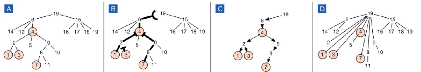
To understand the benefits of path compression, consider a concrete example in Figure 1A, which shows a union-find treeT that is a typical in a union-find forest. The root ofT isr “ 19. Suppose we need to
Algorithm 4:Bulk-FindpU,Sq—find the root inUfor eachsPS with path compression.
Input:Uis the union find structure. Fori“1, . . . ,|S|,Srisis a vertex in the graph
Output: A response arrayresof length|S|whereresrisis the root of the tree of the vertexSrisin the input.
B Phase I:Find the roots for all queries 1: R0Ð xpSrks,nullq : k“0,1,2, . . . ,|S| ´1y
2: F0ÐmkFrontierpR0,Hq,rootsÐ H,visitedÐ H,iÐ0 3: whileRi,Hdo
4: visitedÐvisitedYFi
5: Ri`1Ð xpparentrvs,vq : vPFiandparentrvs,vy
6: rootsÐrootsY tv : vPFiwhereparentrvs “vu
7: Fi`1ÐmkFrontierpRi`1,visitedq,iÐi`1
B Set up response distribution
8: Create an instance ofRDwithRY“R0‘R1‘ ¨ ¨ ¨ ‘Ri
B Phase II:Distribute the answers and shorten the paths 9: D0Ð tpr,rq : rProotsu,iÐ0
10: whileDi,Hdo
11: For eachpv,rq PDi, in parallel,parentrvs Ðr
12: Di`1Ð Ť
pv,rqPDitpu,rq : uPRD.allFrompvqandu,nullu. That is, createDi`1by expanding every
pv,rq PDias the entries ofRD.allFrompvqexcludingnull, each inheritingr.
13: iÐi`1
14: Fori“0,1,2. . . ,|S| ´1, in parallel, makeresris ÐparentrSriss
15: returnres
defmkFrontierpR,visitedq:
//nodes to go to next
1: reqÐ xv : pv,_q PR^ notvisitedrvsy 2: returnremoveDuppreqq
supportfind’s fromu“1 andv“7. When all is done, bothfindpuqandfindpvqshould returnr. Notice that in this example, the paths to the rootu randv rmeet at common vertexw“4. That is, the two paths are identical fromwonward tor. Iffind’s were done sequentially, sayfindpuqbeforefindpvq, then
findpuq—with path compression—would update all nodes on theu rpath to point tor. This means that whenfindpvqtraverses the tree, the path to the root is significantly shorter: forfindpvq, the next hop afterw
is alreadyr.
The kind of sharing and shortcutting illustrated, however, is not possible when thefindoperations are run independently in parallel. Eachfind, unaware of the others, will proceed all the way to the root, missing out on possible sharing.
We fix this problem by organizing the parallel computation so that the work on different “flows” offinds is carefully coordinated. Algorithm 4 shows an algorithmBulk-Find, which works in two phases, separating actions that only read from the tree from actions that only write to it:
B Phase I:Find the roots for all queries, coalescing flows as soon as they meet up. This phase should be thought of as running breadth-first search (BFS), starting from all the query nodesS at once. As with normal BFS, if multiple flows meet up, only one will move on. Also, if a flow encounters a node that has been traversed before, that flow no longer needs to go on. To proceed to Phase II, we need to record the paths traversed so that we can distribute responses to the requesting nodes.
B Phase II:Distribute the answers and shorten the paths. Using the transcript from Phase I, Phase II makes sure that all nodes traversed will point to the corresponding root—and answers delivered to all thefinds. This phase, too, should be thought of as running breadth-first search (BFS) backwards from all the roots reached in Phase I. This BFS reverses the steps taken in Phase I using the trails recorded. There is a technical challenge in implementing this. Back in Phase I, to minimize the cost of recording these trails, the trails are kept as a list of directed edges (marked by their two endpoints) traversed. However, for the reverse traversal
in Phase II to be efficient, it needs a means to quickly look up all the neighbors of a vertex (i.e., at every node, we must be able to find every flow that arrived at this node back in Phase I). For this, we design a data structure that takes advantage of hashing and integer sorting (Theorem 1) to keep the parallel complexity low. We discuss our solution to this problem in the section that follows (Lemma 9).
Example: We illustrate how theBulk-Find algorithm works using the union-find from Figure 1A. The
queries to theBulk-Findare nodes that are circled. The paths traversed in Phase I are shown in panel B. If a flow is terminated, the last edge traversed on that flow is rendered as .
Notice that as soon as flows meet up, only one of them will carry on. In general, if multiple flows meet up at a point, only one will go on. Notice also that both the flow 1Ñ2Ñ4 and the flow 7Ñ8Ñ9Ñ4 are stopped at 4 because 4 is a source itself, which was started at the same time as 1 and 7. At the finish of Phase I, the graph (in fact a tree) given byRYis shown in panel C. Finally, in Phase II, this graph is traversed
and all nodes visited are updated to point to their corresponding root (as shown in panel D).
19 6 15 16 17 18 12 4 14 19 2 5 9 1 3 8 10 7 11 19 6 15 16 17 18 12 4 14 19 2 5 9 1 3 8 10 7 11 19 6 15 16 17 18 12 4 14 19 2 5 9 1 3 8 10 7 11 19 6 4 2 9 1 3 8 7 A B C D
Figure 1:A: An example union-find tree with sample queries circled;B: Bolded edges are paths, together with their
stopping points, that result from the traversal in Phase I;C: The traversal graphRYrecorded as a result of Phase I; and
D: The union-find tree after Phase II, which updates all traversed nodes to point to their roots.
5.1 Response Distributor
Consider a sequenceRY“ xpfromi,toiqyλi“1. We need a data structureRDsuch that after some preprocessing ofRY, can efficiently answer the queryRD.allFrompfqwhich returns a sequence containing alltoiwhere
fromi “ f.
To meet the overall running time bound, the preprocessing step cannot take more thanOpλqwork and
Oppolylogpλqqdepth. As far as we know, we cannot afford to generate, say, a sequence of sequencesRD
whereRDrfsis a sequence containing alltoisuch thatfromi “ f. Instead, we propose a data structure with the following properties:
Lemma 9 (Response Distributor) There is a data structure response distributor (RD) that from input
RY“ xpfromi,toiqyλi“1can be constructed in Opλqwork and Oppolylogpnqqdepth. EachallFromquery can
be answered in Oplogλqdepth. Furthermore, ifFis the set of unique fromi(i.e.,F“ tfromi : i“1, . . . , λu), then E « ÿ fPF WorkpRD.allFrompfqq ff “Opλq.
Proof: Let hbe a hash function from the domain offromi’s (a subset of rns) torρs, whereρ “ 3λ. To construct anRD, we proceed as follows. Compute the hash for eachfromiusinghp¨qand sort the ordered pairspfromi,toiqby their hash values. Call this sorted arrayA. After sorting, we know that pairs with the same hash value are stored consecutively inA. Now create an arrayoof lengthρ`1 so thatoi marks the beginning of pairs whose hash value isi. If none of them hash toi,oi “oi`1. These steps can be done using
intSortand standard techniques inOpλqwork andOppolylogpλqqdepth because the hash values range withinOpλq.
To supportallFrompfq, we computeκ“hpfqand look inAbetweenoκandoκ`1´1, selecting only
pairs whosefrommatches f. This requires at mostOplog|oκ`1´oκ|q “Oplogλqdepth. The more involved question is how much work is needed to supportallFromover all. To answer this, consider all the pairs in
RYwithfromi “ f. Letnf denote the number of such pairs. Thesenf pairs will be gone through by queries looking for f and other entries that happen to hash to the same value as f does. The exact number of times these pairs are gone through isβf :“#tsPF:hpfq “hpsqu. Hence, across all queries f PF, the total work
isřfPFnfβf. ButE “ βf ‰ ď1`|Fρ|, so ÿ fPF E“nfβf ‰ ď ´ 1`|Fρ|¯ ÿ fPF nf ď p1`3λλqλď2λ
because|F| ďλandřfPFnf “λ, completing the proof.
With this lemma, the cost ofBulk-Findcan be stated as follows.
Lemma 10 Bulk-FindpU,Sqdoes Op|RY|qwork and has Oppolylogpnqqdepth.
Proof: The Ri’s, Fi’s, and Di’s can be maintained directly as arrays. Theroots andvisited sets can be maintained as as bit flags on top of the vertices ofU as all we need are setting the bits (adding/removing elements) and reading their values (membership testing). There are two phases in this algorithm. In Phase I, the cost of addingFitovisitedin iterationiis bounded by|Ri|. Using standard parallel operations [11], the work of the other steps is clearly bounded by|Ri`1|, includingmkFrontierbecauseremoveDupdoes work
linear in the input, which is bounded by|Ri`1|. Thus, the work of Phase I is at mostOp
ř
i|Ri|q “Op|RY|q.
In terms of depth, because the union-find tree has depth at mostOplognq, thewhileloop can proceed for at mostOplognqtimes. Each iteration involves standard operations with depth at mostOplog2nq, so the depth of Phase I is at mostOplog3nq.
In Phase II, the dominant cost comes from expandingDiintoDi`1by callingRD.allFrom. By Lemma 9,
across all iterations, the work caused byRD.allFrom, run on each vertex once, is expectedOp|RY|q, and the depth is Oppolylogp|RY|qq ď Oppolylogp|RY|qq. Overall, the algorithm requiresOp|RY|q work and
Oppolylogpnqqdepth.
5.2 Bulk-Find’s Cost Equivalence to Serialfind
In analyzing the work bound of the improved data structure, we will show that whatBulk-Finddoes is equivalent to some sequential execution of the standardfindand requires the same amount of work, up to constants.
To gather intuition, we will manually derive such a sequence for the sample queries S “ t1,3,4,7u used in Figure 1. The query of 4 went all the way to the root without merging with another flow. But the queries of 1 and 7 were stopped at 4 and in this sense, depended upon the response from the query of 4. By the same reasoning, because the query of 3 merged with the query of 1 (with 1 proceeding on), the query of 3 depended on the response from the query of 1. Note that in this view, although the query of 3 technically waited for the response at 2, it was the query of 1 that brought the response, so it depended on 1. To derive a sequence execution, we need to respect the “depended on” relation: ifadepended onb, thena
will be invoked afterb. As an example, one sequential execution order that respects these dependencies is
findp4q,findp7q,findp1q,findp3q.
We can check that by applying finds in this order, the paths traversed are exactly what the parallel execution does asU.findperforms full path compression.
We formalize this idea in the following lemma:
Lemma 11 For a sequence of queries S with whichBulk-FindpU,Sqis invoked, there is a sequence S1that
is a permutation S such that applying U.findto S1 serially in that order yields the same union-find forest
asBulk-Find’s and incurs the same traversal cost of Op|RY|q, where RYis as defined in theBulk-Find
algorithm.
Proof: For this analysis, we will associate everypparent,childq PRYwith a queryqPS. Logically, every queryq P S starts a flow atqascending up the tree. If there are multiple flows reaching the same node,
removeDup inside mkFrontierdecides which flow to go on. From this view, for any nonroot node u
appearing inRY, there isexactlyone query flow from this node that proceeds up the tree. We will denote this flow byownpuq.
If a query flow is stopped partway (without reaching the corresponding root), the reason is either it merges in with another flow (viamkFrontier) or it recognizes another flow that visited where it is going before (via
visited). For every queryqthat is stopped partway, letrpqqbe the furthest point in the tree it has advanced to, i.e.,rpqqis the endpoint of the maximal path inRYfor the query flowq.
In this set up, a query flow whose furthest point isuwill depend on the response from the queryownpuq. Therefore, we form a dependency graphGdep(“udepends onv”) as follows. The vertices are all the vertices fromS. For every query flowqthat is stopped partway, there is an arcownprpqqq Ñq.
LetS1be a topologically-ordered sequence ofG
dep. Multiple copies of the same query vertex can simply be placed next to each other. If we applyU.findserially onS1, then all queries that a query vertexqdepends on inGdep will have been called prior toU.findpqq. Because of full path compression, this means that
U.findpqqwill followu rpqq Ñ t(rpqq Ñtis one step), wheretis the root of the tree. Hence, every
U.findpqqtraverses the same number of edges asu rpqqplus 1. As everyRYedge is part of a query flow,
we conclude that the work of runningU.findonS1in that order isOp|R
Y|q.
Finally, to obtain the bounds in Theorem 8, we modifySimple-Bulk-QueryandSimple-Bulk-Update
(in the relabeling step) to useBulk-Findon all query pairs. The depth clearly remainsOppolylogpnqqper bulk operation. Aggregating the cost ofBulk-Findacross calls fromBulk-UpdateandBulk-Query, we know from Lemma 11 that there is a sequential order that has the same work. Therefore, the total work is bounded byOppm`qqαpm`q,nqq.
6
Implementation and Evaluation
This section discusses an implementation of the proposed data structure and its empirical performance.
6.1 Implementation
With an eye toward a simple implementation that delivers good practical performance, we set out to implement the simple bulk-parallel data structure from Section 4. The underlying union-find data structureUmaintains two arrays of lengthn—parentandsizes—one storing a parent pointer for each vertex, and the other tracking the sizes of the trees. Thefindandunionoperations follow a standard textbook implementation.
On top of these operations, we implementedSimple-Bulk-QueryandSimple-Bulk-Updateas described earlier in the paper. We use standard sequence manipulation operations (e.g., filter, prefix sum, pack, remove duplicate) from the PBBS library [16]. There are two modifications that we made to improve practical performance of the implementation:
Path Compression:We wanted some benefits of path compression but without the full complexity of the work-efficient parallel algorithm from Section 5, to keep the code simple. We settled with the following pragmatic solution: Thefindoperations insideSimple-Bulk-QueryandSimple-Bulk-Updatestill run independently in parallel. But after finding the root, each operation traverses the tree one more time to update all the nodes on the path to point to the root. This leads to shorter paths for later bulk operations with clear performance benefits. However, for large bulk sizes, the approach may still perform significantly more work than the work-efficient solution because the path compression from afindoperation may not benefit other
findoperations within the same minibatch.
Connected Components:The algorithm as described uses as a subroutine a linear-work parallel algorithm to find connected components. These linear work algorithms expect a graph representation that gives quick random access to the neighbors of a vertex. We found the processing cost to meet this requirement to be very high and instead implemented the algorithm for connectivity described in Blelloch et al. [3]. Although this has worse theoretical guarantees, it can work with a sequence of edges directly and delivers good real-world performance.
6.2 Experimental Setup
Environment:We performed experiments on an Amazon EC2 instance with 20 cores (allowing for 40 threads
via hyperthreading) of 2.4 GHz Intel Xeon E5-2676 v3 processors, running Linux 3.11.0-19 (Ubuntu 14.04.3). We believe this represents a baseline configuration of midrange workstations available in a modern cluster. All programs were compiled with Clang version 3.4 using the flag-O3. This version of Clang has the Intel Cilk runtime, which implements a work-stealing scheduler known to impose only a small overhead on both parallel and sequential code. We report wall-clock time measured usingstd::chrono::high_resolution_clock.
For robustness, we performthreetrials and report the median running time. Although there is randomness involved in the connected component (CC) algorithm, we found no significant fluctuations in the running time across runs.
Datasets:Our study aims to study the behavior of the algorithm on a variety of graph streams. To this end,
we use a collection of synthetic graph streams created using well-accepted generators. We include both power-law-type graphs and more regular graphs in the experiments. These are graphs commonly used in dynamic/streaming graph experiments (e.g., [13]). A summary of these datasets appear in Table 1.
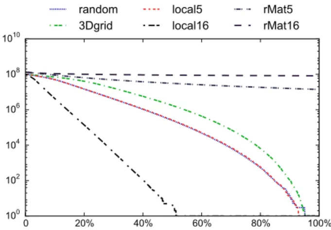
The graph streams in our experiments differ substantially in how quickly they become connected. This input characteristic influences the data structure’s performance. In Figure 2, we show for each graph stream, the number of connected components at different points in the stream. The local16 graph becomes fully connected right around the midpoint of the stream. Both rMat5 and rMat16 continue to have tens of millions of components after consuming the whole stream. Note that in this figure, random and local5 are almost visually indistinguishable until the very end.
Baseline:We directly compare our algorithms with union find (denotedUF), using both the union by size
and a path compression variant, which has the optimal sequential running time. Most prior algorithms either focus on parallel graphs or streaming graphs, not parallel streaming graphs. We note that the algorithm of McColl et al. [13] that works in the parallel dynamic setting is not directly comparable to ours. Their
Graph #Vertices #Edges Notes
3Dgrid 99.9M 300M 3-d mesh
random 100M 500M 5 randomly-chosen neighbors per
node
local5 100M 500M small separators, avg. degree 5
local16 100M 1.6B small separators, avg. degree 16
rMat5 134M 500M power-law graph using rMat [4]
rMat16 134M 1.6B a denser rMat graph
Table 1:Characteristics of the graph streams used in our experiments, showing for every dataset, the total number of nodes (n), the total number of edges (m), and a brief description.
0 20% 40% 60% 80% 100% 100 102 104 106 108 1010 random 3Dgrid local5 local16 rMat5 rMat16
Figure 2:The numbers of connected components for each graph dataset at different percentages of the total graph stream processed.
algorithm focuses on supporting insertion and deletion of arbitrary edges, whereas ours is designed to take advantage of the insert-only setting.
6.3 Results
How does the bulk-parallel data structure perform on a multicore machine? To this end, we investigate the parallel overhead, speedup, and scalability trend.
Table 2 shows the timings for the baseline sequential implementation of union-findUFwith and without path compression and the bulk-parallel implementationon a single thread for four different batch sizes, 500K, 1M, 5M, and 10M. To measure overhead, we first compare our implementation to union findwithout
path compression: our implementation is between 1.01x and 2.5x slower except on local16, in which the bulk parallel achieves some speedups even on one thread. This is mainly because the number of connected components in local16 drops quickly to 1 as soon as midstream (Figure 2). With only 1 connected component, there is little work for bulk-parallel to be done after that. Compared to union find with path compression, our implementation, which does pragmatic path compression, shows nontrivial—but still acceptable—overhead, as to be expected because our solution does not fully benefitfinds within the same minibatch.
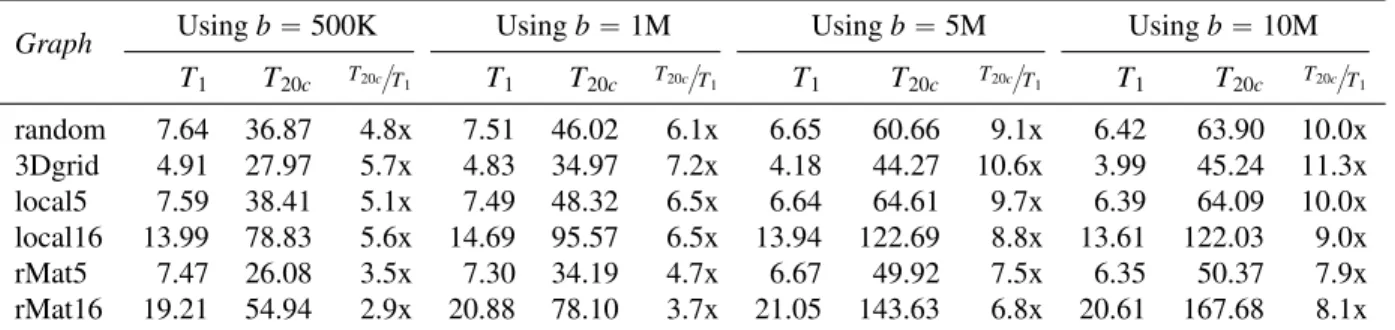
Table 3 shows the average throughputs (million edges/second) ofBulk-Updatefor different batch sizes. HereT1denotes the throughput on 1 thread andT20c the throughput on 20 cores (40 hyper-threads). We also show the speedup as measured byT20c{T1. We observe consistent speedup on all six datasets under all four
Graph UF UF Bulk-Parallel Using Batch Size (no p.c.) (p.c.) 500K 1M 5M 10M random 44.63 18.42 65.43 66.57 75.20 77.89 3Dgrid 30.26 14.37 61.10 62.00 71.74 75.07 local5 44.94 18.51 65.84 66.77 75.33 78.23 local16 154.40 46.12 114.34 108.92 114.80 117.55 rMat5 33.39 18.47 66.98 68.48 74.97 78.69 rMat16 81.74 35.29 83.27 76.64 76.03 77.62
Table 2:Running times (in seconds) on 1 thread of the baseline union-find implementationUFwith and without path
compression (unaffected by the batch size) and the bulk-parallel data structure as the batch size is varied.
Graph Usingb“500K Usingb“1M Usingb“5M Usingb“10M
T1 T20c T20c{T1 T1 T20c T20c{T1 T1 T20c T20c{T1 T1 T20c T20c{T1 random 7.64 36.87 4.8x 7.51 46.02 6.1x 6.65 60.66 9.1x 6.42 63.90 10.0x 3Dgrid 4.91 27.97 5.7x 4.83 34.97 7.2x 4.18 44.27 10.6x 3.99 45.24 11.3x local5 7.59 38.41 5.1x 7.49 48.32 6.5x 6.64 64.61 9.7x 6.39 64.09 10.0x local16 13.99 78.83 5.6x 14.69 95.57 6.5x 13.94 122.69 8.8x 13.61 122.03 9.0x rMat5 7.47 26.08 3.5x 7.30 34.19 4.7x 6.67 49.92 7.5x 6.35 50.37 7.9x rMat16 19.21 54.94 2.9x 20.88 78.10 3.7x 21.05 143.63 6.8x 20.61 167.68 8.1x
Table 3: Average throughput (in million edges/second) and speedup of Bulk-Updatefor different batch sizesb,
whereT1is throughput on 1 thread andT20cis the throughput on 20 cores.
This is to be expected, since a larger batch size means more work per core in processing each batch, and lesser overhead of synchronization.
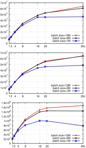
Figure 3 shows the average throughput (edges/sec) as the number of threads increases from 1 to 20c, which represents 40 hyperthreads. Three different batch sizes were used for the experiments: 1M, 5M and 10M. The top chart represents the results on the random dataset, the middle chart on the local16 dataset and the bottom chart on the rMat16 dataset. In general, as the number of threads increases, the average throughput increases for all 3 datasets under different batch sizes. With a 10M batch size on 20 cores, we observe speedups between 8–11x. On the rMat16 dataset (the bottom chart), the throughput starts to drop with batch size of 1M when the number of threads increases beyond 20. This is due to the relatively large number of connected components in the rMat16 dataset from the beginning towards the end of processing the entire dataset(see Figure 2). In this case, the work done per batch of input edges is relatively small, and a 1M batch size is too small for the rMat16 dataset to realize additional parallelization benefits beyond 20 threads.
7
Conclusion
We presented a shared-memory parallel algorithm for incremental graph connectivity in the minibatch arrival model. Our algorithm has polylogarithmic parallel depth and its total work across all processors is of the same order as the work due to the best sequential algorithm for incremental graph connectivity. We also presented a simpler parallel algorithm that is easier to implement and has good practical performance.
This presents several natural open research questions. We list some of them here. (1) In case all edge updates are in a single minibatch, the total work of our algorithm is (in a theoretical sense), superlinear in
0 1x10⁷ 2x10⁷ 3x10⁷ 4x10⁷ 5x10⁷ 6x10⁷ 7x10⁷ 1 2 4 8 16 20 20c batch size=10M batch size=5M batch size=1M 0 1x10⁷ 2x10⁷ 3x10⁷ 4x10⁷ 5x10⁷ 6x10⁷ 7x10⁷ 1 2 4 8 16 20 20c batch size=10M batch size=5M batch size=1M 0 2x10⁷ 4x10⁷ 6x10⁷ 8x10⁷ 1x10⁸ 1.2x10⁸ 1.4x10⁸ 1.6x10⁸ 1.8x10⁸ 1 2 4 8 16 20 20c batch size=10M batch size=5M batch size=1M
Figure 3:Average throughput (edges per second) as the number of threads is varied from 1 to 40 (denoted by 20cas they run on 20 cores with hyperthreading). The graph streams shown are (top) random, (middle) local16, and (bottom) rMat16.
the number of edges in the graph. Whereas, the optimal batch algorithm for graph connectivity, based on a depth-first search, has work linear in the number of edges. Is it possible to have an incremental algorithm whose work is linear in the case of very large batches, such as the above, and falls back to the union-find type algorithms for smaller minibatches? Note that for all practical purposes, the work of our algorithm is linear in the number of edges, due to very slow growth of the inverse Ackerman’s function. (2) Can these results on parallel algorithms be extended to the fully dynamic case when there are both edge arrivals as well as deletions?
References
[1] Richard J. Anderson and Heather Woll. Wait-free parallel algorithms for the union-find problem. In
Proceedings of the 23rd Annual ACM Symposium on Theory of Computing, May 5-8, 1991, New Orleans, Louisiana, USA, pages 370–380, 1991.
[2] Jonathan Berry, Matthew Oster, Cynthia A. Phillips, Steven Plimpton, and Timothy M. Shead. Main-taining connected components for infinite graph streams. InProc. 2nd International Workshop on Big Data, Streams and Heterogeneous Source Mining: Algorithms, Systems, Programming Models and Applications (BigMine), pages 95–102, 2013.
[3] Guy E. Blelloch, Jeremy T. Fineman, Phillip B. Gibbons, and Julian Shun. Internally deterministic parallel algorithms can be fast. InProceedings of the 17th ACM SIGPLAN Symposium on Principles and Practice of Parallel Programming, PPOPP 2012, New Orleans, LA, USA, February 25-29, 2012, pages 181–192, 2012.
[4] Deepayan Chakrabarti, Yiping Zhan, and Christos Faloutsos. R-MAT: A recursive model for graph mining. InProceedings of the Fourth SIAM International Conference on Data Mining, Lake Buena Vista, Florida, USA, April 22-24, 2004, pages 442–446, 2004.
[5] Thomas H. Cormen, Charles E. Leiserson, Ronald L. Rivest, and Clifford Stein. Introduction to Algorithms (3. ed.). MIT Press, 2009.
[6] Camil Demetrescu, Bruno Escoffier, Gabriel Moruz, and Andrea Ribichini. Adapting parallel algorithms to the W-stream model, with applications to graph problems. Theor. Comput. Sci., 411(44-46):3994– 4004, 2010.
[7] Camil Demetrescu, Irene Finocchi, and Andrea Ribichini. Trading off space for passes in graph streaming problems. ACM Transactions on Algorithms, 6(1), 2009.
[8] Joan Feigenbaum, Sampath Kannan, Andrew McGregor, Siddharth Suri, and Jian Zhang. On graph problems in a semi-streaming model. Theor. Comput. Sci., 348(2-3):207–216, 2005.
[9] Hillel Gazit. An optimal randomized parallel algorithm for finding connected components in a graph.
SIAM J. Comput., 20(6):1046–1067, 1991.
[10] IBM Corporation. Infosphere streams. http://www-03.ibm.com/software/products/en/
infosphere-streams. Accessed Jan 2014.
[12] Bruce M. Kapron, Valerie King, and Ben Mountjoy. Dynamic graph connectivity in polylogarithmic worst case time. InProceedings of the Twenty-Fourth Annual ACM-SIAM Symposium on Discrete Algorithms, SODA 2013, New Orleans, Louisiana, USA, January 6-8, 2013, pages 1131–1142, 2013. [13] Robert McColl, Oded Green, and David A. Bader. A new parallel algorithm for connected components
in dynamic graphs. In20th Annual International Conference on High Performance Computing, HiPC 2013, Bengaluru (Bangalore), Karnataka, India, December 18-21, 2013, pages 246–255, 2013. [14] Sanguthevar Rajasekaran and John H. Reif. Optimal and sublogarithmic time randomized parallel
sorting algorithms. SIAM J. Comput., 18(3):594–607, 1989.
[15] Raimund Seidel and Micha Sharir. Top-down analysis of path compression.SIAM J. Comput., 34(3):515– 525, 2005.
[16] Julian Shun, Guy E. Blelloch, Jeremy T. Fineman, Phillip B. Gibbons, Aapo Kyrola, Harsha Vardhan Simhadri, and Kanat Tangwongsan. Brief announcement: the problem based benchmark suite. In24th ACM Symposium on Parallelism in Algorithms and Architectures, SPAA ’12, Pittsburgh, PA, USA, June 25-27, 2012, pages 68–70, 2012.
[17] Julian Shun, Laxman Dhulipala, and Guy E. Blelloch. A simple and practical linear-work parallel algorithm for connectivity. In26th ACM Symposium on Parallelism in Algorithms and Architectures, SPAA ’14, Prague, Czech Republic, pages 143–153, 2014.
[18] Robert Endre Tarjan. Efficiency of a good but not linear set union algorithm. Journal of the ACM, 22(2):215–225, 1975.
[19] M. Zaharia, T. Das, H. Li, T. Hunter, S. Shenker, and I. Stoica. Discretized streams: Fault-tolerant streaming computation at scale. InProc. ACM Symposium on Operating Systems Principles (SOSP), pages 423–438, 2013.