Bayesian Forecasting of Stock Prices Via the Ohlson Model

(1)

Bayesian Forecasting of Stock Prices

Via the Ohlson Model

By

Qunfang Flora Lu

A Thesis

Submitted to the Faculty of

WORCESTER POLYTECHNIC INSTITUTE in partial fulfillment of the requirements for the

Degree of Master of Science in

Applied Statistics by

May 2005

APPROVED:

Balgobin Nandram, Professor and major advisor

Huong Higgins, Associate Professor and co-advisor

(2)

Abstract

Over the past decade of accounting and finance research, the Ohlson (1995) model has been widely adopted as a framework for stock price prediction. While using the accounting data of 391 companies from SP500 in this paper, Bayesian statistical techniques are adopted to enhance both the estimative and predictive qualities of the Ohlson model comparing to the classical approaches. Specifically, the classical methods are used for the exploratory data analysis and then the Bayesian strategies are applied using Markov chain Monte Carlo method in three stages: individual analysis for each company, grouping analysis for each group and adaptive analysis by pooling information across companies. The base data, which consist of 20 quarters’ observations starting from the first quarter of 1998, are used to make inferences for the regression coefficients (or parameters), evaluate the model adequacy and predict the stock price for the first quarter of 2004, when the real observations are set as the test data to evaluate the predictive ability of the Ohlson model. The results are averaged within each specified group categorized via the general industrial classification (GIC). The empirical results show that classical models result in larger stock price prediction errors, more positively-biased predictions and have much smaller explanatory powers than Bayesian models. A few transformations of both classical and Bayesian models are also performed in this paper, however, transformations of the classical models do not outweigh the usefulness of applying Bayesian statistics.

(3)

Acknowledgements

I would like to express my deep gratitude to the following people for their academic, financial or spiritual support in finishing this thesis.

Advisors: Balgobin Nandram and Huong Higgins. Without their help and guidance, there would not have been such a piece of work. There are no words that can express the appreciation from the bottom of my heart to them. And I promise this is not the end of my devotion to the research on this topic. I will keep in touch with them wherever I am.

Professors in the Math Department of WPI: Joseph D. Petruccelli, Jayson Wilbur, Andrew Swift, Carlos Morales and Christopher J. Larsen. Their courses have strengthened my knowledge in Applied Statistics and Applied Math. Also thank to Mayer Humi, William W. Farr, John Goulet, Dalin Tang, Peter R. Christopher and William J. Martin for their guidance in my two years of working experience as a teaching assistant.

Secretaries in the Math Department of WPI: Colleen Lewis, Ellen Mackin, Deborah Riel. They are the nicest, most patient and helpful secretaries that I’ve ever seen. Best wishes to them forever!

My parents and brother: Zhongxiao Lu, Rongzhi Liu, Hanliang Lu. They are always there when I’m in need; they accept me when I’m rejected; they are still proud of me even when I do not feel any good about a single part of myself.

My fiancé and his family: John Cacka, Bethlynne Vanella and Jennifer Graham etc. They gave me a warm home when I was in the hardest time in USA, and have been supporting me even since then. They like Chinese, I love them.

WPI Ballroom Dance Team: Boris Mosis and Miles Schofield etc. They helped me develop a terrific hobby --- dancing, which is my life, my soul and my best joy in the free time. Thanks for all those exciting practice lessons and dance parties.

(4)

Colleagues and classmates: Fang Huang, Yan Bai, Guochun Liu, Alina Ursan, Shinji Uemura, Gregory Matthews, Shawn Hallinan, Ashley Moraski, Rajesh Kondapaneni, Jasraj Kohli, Daniel Onofrei, Bijaya Padhy, Elizabeth Teixeira and Scott Laine etc. I had fun discussing homework problems with them. Sometimes we also talked about life, worries and future dreams. They are nice, smart and very friendly. I will keep them in my memory.

Friends: Jeani Lu, Mark Bertolina, Alin Sirbu, Congmei Ma, Chi Hu, Pong Pang, Fang Liu, Yucong Huang, Qunwei Ai, Chao Ku and Xiaolin Nan etc. They are not many, but enough to make me a rich and confident woman.

Last but not least, to those who doubt my intelligence, willpower and potential. I will fan the flame of dissatisfaction and make a miracle to them, to myself and to this wonderful world.

(5)

Chapter 1

The Ohlson (1995) Model and Data of S&P 500

1.1 The Ohlson (1995) Model

Over the past two decades in finance and accounting area, considerable attention has been paid to the relationship between accounting numbers (book values, earnings, etc.) and the firm value. The Ohlson (1995) approach to the problem of stock valuation relates

securities prices to accounting data, and provides a structure for applicable modeling. The Ohlson (1995) Valuation Model has been widely adopted by researchers and practitioners on profitability analysis as a framework for the fundamental valuation of equities. It also has been developed into several versions, e.g., Feltham-Ohlson (1995) Valuation Model, Bernard’s (1995) Ohlson Approximation Model, Liu-Ohlson (2000) Valuation Model and Callen’s (2001) Ohlson AR(2) Valuation Model. For a historical development process of the Ohlson model, see Appendix A.

This paper evaluates the Ohlson (1995) Forecasting Model (OFM), or briefly the Ohlson (1995) model, and uses it to forecast stock prices. OFM is a practicable case of Bernard’s (1995) Ohlson Approximation Model (see Appendix C). For a single firm, OFM states: the stock price per share is a linear function of the company’s book value per share and abnormal earnings per share for the following four periods with normally distributed innovation terms, which represents “other information” whose source is uncorrelated with abnormal earnings. In mathematical form, it can be expressed as

, , , 1 , 4 3 2 1 , ~ ' ~ 4 1 2 2 1 T t , , , k v x v x bv y _t t t k a k t k t t  = = + = + + + =

∑

= + + β β β β (1.1.1)

where yt denotes the stock price per share at time t, bvt is the book value per share at time t, a

t

x represents the abnormal earning at time t, ( 1, 6)'

~ β β

(6)

intercept and slope coefficients of the predictors, (1, , 1, 2, 3, 4)' ' ~ a t a t a t a t t t bv x x x x x = ₊ ₊ ₊ ₊ is the

vector of intercept and predictors, and vt is the innovation (error or residual) term.

To understand the “abnormal earning” term, we can view it as a contraction of “above normal earning”. Ohlson (1995) proposes the abnormal earning as

= t − t t₋₁, a

t x rbv

x (1.1.2) wherext is the earning per share at time t for a company, rt is the discount rate at time t.

Since the values of the following four periods ( ₁, ₂, ₃, a₄) t a t a t a t x x x

x₊ ₊ ₊ ₊ are used to forecast the stock price, this paper uses the expected earnings to replace xt in (1.1.2). That is,

= [ t]− t t−1

a

t E x rbv

x . (1.1.3)

For the innovation term, Ohlson (1995) assumes it has a first order autoregressive structure (AR(1)). This assumption can be described as

), , 0 ( ~ , 2 1 σ ε ε ρ N v v t t t t = − + (1.1.4)

whereρ is the correlation coefficient of time series vt, εt is the white noise, σ2 is the variance of the white noise. Note that if ρ <1, the AR(1) process is stationary.

From (1.1.1) and (1.1.4) we can get

, ~ ' 1 ~ 1 1 β − − − = t − _t t y x v . , ~ ' 1 ~ 1 ~ ' ~ ~ ' 1 ~ 1 1 t t t t t t t t t t t x y x y x y v v ε β ρ β ε β ρ ε ρ +     ₋ + = +     ₋ = + = − − − − −

(7)

But whent =1, 1 ~ ' 0 ~ 0 ~ ' 1 ~ 1 = x β+ρy −x β+ε

y , there exists unobserved values y0 and

' 0 ~

x _.

This paper lets = _ − _

~ ' 0 ~ 0 β ρ

µ y x . Therefore, expressions (1.1.1) and (1.1.4) can be combined as , , , 1 ), , 0 ( ~ , , , 2 , ) ( , 2 ~ ' 1 1 ~ ' 1 ~ ' 1 1 T t N T t x y x y x y iid t t t t t t   = = + − + = + + = − − σ ε ε β ρ β ε µ β (1.1.5)

whereµ, ρ and_σ2_{are three unknown parameters besides the intercept and regression}

coefficients in

~

β_.

Expression (1.1.5) is the complete form of the Ohlson (1995) Forecasting Model, hereinafter the Ohlson model, that is used in this paper.

1.2 Retrieving Data of S&P 500 from Thomson ONE Analytics

Yearly or quarterly data from various sources have been applied to test the Ohlson model. For instances, besides many tests that use US data, Bao & Chow (1999) test the

usefulness of the Ohlson model using data from listed companies in the People’s

Republic of China; McCrave & Nilsson (2001) compare the difference between Swedish and US firms by using data from a Swedish business magazine, Bonnier-Findata database and I/B/E/S database; Ota (2002) uses empirical evidence from Japan, etc. This paper applies quarterly data of S&P 500 from Thosmon ONE Analytics to the Ohlson model.

S&P 500 is one of the most widely used measures of U.S. stock market performance and is considered to be a bellwether for the U.S. economy. S&P refers to Standard & Poor’s, which is a division of the McGraw-Hill Companies, Inc. 500 companies are selected among the leaders in the major industries driving U.S. economy by the S&P Index

(8)

Committee for market size, liquidity and sector representation. A small number of international companies that are widely traded in the U.S are included.

The needed data of S&P 500 can be retrieved from Thomson ONE Analytics by its Excel Add-in software, provided by the Thomson Corporation, which is a global leader in providing value-added information, software applications and tools in the fields of law, tax, accounting, financial services and corporate training and assessment etc. Thomson ONE Analytics is a web based application that allows users to research information about different companies and markets, including current stock prices, volume traded, EPS (expected earning per share) and so on. The “Thomson ONE Analytics Excel Add-in” is one of the most valuable features that Thomson ONE Analytics offers its users. Using the Add-in, financial analysts can pull data directly into Excel from a wealth of financial databases such as “Worldscope”, “Compustat”, “U.S. Pricing”, “I/B/E/S and I/B/E/S History” and “Extel” by using the powerful PFDL (Premier Financial Database Language).

Items in the retrieved data are: Total Assets, Total Liabilities, Preferred Stock, Common Shares Outstanding from database “Worldscope”; “EPSmeanQTR1-4” and

“EPSConsensusForecastPeriodQTR1-4” from database “I/B/E/S History” (note that these are monthly data); Dow Jones Industry Group (DJIC), General Industry Classification (GIC), Dow Jones Market Sector (DJMS) and GICSSECTOR from “Thomson

Financial”; PriceClose and 3-month T-bill (treasury bill) rate from “Datastream”. Book value per common share (BPS) can be calculated by the first four items in following formula:

BPS = (Total Assets − Total Liabilities − Preferred Stock)/(Common Shares Outstanding).

Companies forecast their expected earnings every month for the following four fiscal quarters. This paper uses the latest forecast value for each quarter to represent the corresponding quarter value. The quarterly EPS are extracted from the monthly data of “EPSmeanQTR1-4” and “EPSConsensusForecastPeriodQTR1-4”. For easier use, values

(9)

of Dow Jones Industry Group, Dow Jones Market Sector and the Company Identity Keys are transformed into integers. (For example, use 3104 instead of the original value C000003104.) To understand these financial / accounting terms, please see Appendix D. Appendix E explains how to use Excel Add-in. Appendix F explains how to extract quarterly data out of monthly data.

After deleting all the missing and incomplete data points and the data points that cause programming errors, 391 companies are selected. This final quarterly data set have 21 points for each company, covering 25 quarters from the first quarter of 1998 and the first quarter of 2004. It is formatted into 16 items which are all numerical values and contain 4 sectors (DJIC, GIC, DJMS and GICSSECTOR), company identity key (ID), Time, PriceClose, BPCS0-3, EPS1-4 and R (3-month T-bill rate).

1.3 Exploratory Data Analysis by Classical Approaches

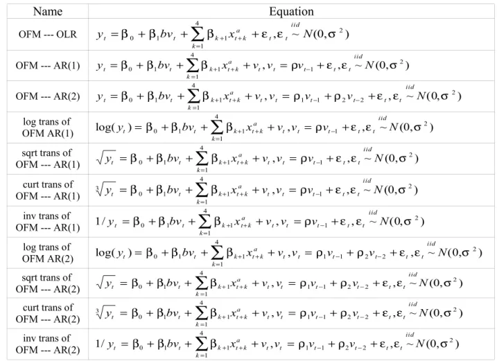
While considering the ideas in various versions of the Ohlson model, this paper sticks to the main frame of the Ohlson model in (1.1.5), and sets up 11 different models which are described in Table 1.3.1 for the exploratory analysis.

These 11 models can be classified into three groups by distinguishing the assumption of the innovation term: independent errors among time periods which belongs to the ordinary linear regression structure (OLR), AR(1) structure for the error and AR(2) structure for the error. The main point of this classification is to check whether the AR(1) assumption is proper for the innovation term of the Ohlson model. Besides this, four kinds of transformation to the term of stock price per share are applied to the model under either AR(1) or AR(2) assumption for the innovation term: logarithmic transformation (log trans), square root transformation (sqrt trans), cubic root transformation (curt trans) and inverse transformation (inv trans). Two relatively better transformations are to be selected by the classical statistical analysis. This paper assumes their priorities to be adopted in further research by the innovative methods, for the reason of their being more fit to the data. The purpose of using transformations is to improve both the estimative

(10)

and predictive qualities of the Ohlson model.

Table 1.3.1 --- Various Models

Name Equation OFM --- OLR 4 , ~ (0, 2) 1 1 1 0 β β ε ε σ β bv x N y t tiid a k t k k t t = + + + + = +

∑

OFM --- AR(1) , , ~ (0, 2) 1 4 1 1 1 0 β β ρ ε ε σ β bv x v v v N y a _t _t _t _t _tiid k t k k t t = + + + + = − + = +

∑

OFM --- AR(2) , , ~ (0, 2) 2 2 1 1 4 1 1 1 0 β β ρ ρ ε ε σ β bv x v v v v N y t t t t t t iid a k t k k t t = + + + + = − + − + = +

∑

log trans of

OFM AR(1) log( ) , 1 , ~ (0, 2)

4 1 1 1 0 β β ρ ε ε σ β bv x v v v N y t t t t tiid a k t k k t t = + + + + = − + = +

∑

sqrt trans of OFM --- AR(1) , 1 , ~ (0, 2) 4 1 1 1 0 β β ρ ε ε σ β bv x v v v N y t t t t tiid a k t k k t t = + + + + = − + = +

∑

curt trans of OFM --- AR(1) , , ~ (0, ) 2 1 4 1 1 1 0 3 _y β β _bv β _x _v _v ρ_v ε ε _N σ iid t t t t t a k t k k t t = + + + + = − + = +

∑

inv trans of OFM --- AR(1) 1/ , 1 , ~ (0, 2) 4 1 1 1 0 β β ρ ε ε σ β bv x v v v N y t t t t t iid a k t k k t t = + + + + = − + = +

∑

log trans of

OFM AR(2) log( ) , 1 1 2 2 , ~ (0, 2)

4 1 1 1 0 β β ρ ρ ε ε σ β bv x v v v v N y t t t t t t iid a k t k k t t = + + + + = − + − + = +

∑

sqrt trans of OFM --- AR(2) , , ~ (0, ) 2 2 2 1 1 4 1 1 1 0 β β ρ ρ ε ε σ β bv x v v v v N y t t t t t tiid a k t k k t t = + + + + = − + − + = +

∑

curt trans of OFM --- AR(2) , , ~ (0, ) 2 2 2 1 1 4 1 1 1 0 3 _y β β_bv β _x _v _v ρ_v ρ _v ε ε iid_N σ t t t t t t a k t k k t t = + + + + = − + − + = +

∑

inv trans of OFM --- AR(2) 1/ , 1 1 2 2 , ~ (0, 2) 4 1 1 1 0 β β ρ ρ ε ε σ β bv x v v v v N y a _t _t _t _t _t _tiid k t k k t t = + + + + = − + − + = +

∑

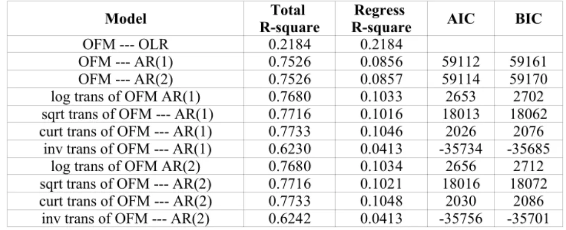
Two procedures, PROC REG and PROC AUTOREG in SAS, are the classical methods that are used to the whole data set to test the estimative ability of the 11 models. Specifically, PROC REG is only used to model OFM---OLR and PROC AUTOREG is used to the models with AR(p) structures for the innovation term. Three kinds of criteria are used to compare their estimative abilities: squares (total square and Regress R-square), Akaike Information Criterion (AIC) and Bayesian Information Criterion (BIC). See Table 1.3.2 for the empirical results. Note that R-square is the coefficient of determination (regression sum of squares divided by total sum of squares). Total R-square is R-R-square and regress R-R-square is R-R-square adjusted for additional covariates. They are nearly the same in PROC REG procedure, but can be very different in PROC AUTOREG procedure, especially when the innovation terms are highly correlated among

(11)

time periods. BIC is a quantity proportional to the negative log likelihood after all parameters are integrated out. AIC is a deviance measure (i.e., difference between observed and fitted models). Models with small AIC and BIC values are preferred.

Table 1.3.2 --- Overall Estimative Ability Comparison of Various Models

Model R-squareTotal R-squareRegress AIC BIC

OFM --- OLR 0.2184 0.2184

OFM --- AR(1) 0.7526 0.0856 59112 59161

OFM --- AR(2) 0.7526 0.0857 59114 59170

log trans of OFM AR(1) 0.7680 0.1033 2653 2702

sqrt trans of OFM --- AR(1) 0.7716 0.1016 18013 18062

curt trans of OFM --- AR(1) 0.7733 0.1046 2026 2076

inv trans of OFM --- AR(1) 0.6230 0.0413 -35734 -35685

log trans of OFM AR(2) 0.7680 0.1034 2656 2712

sqrt trans of OFM --- AR(2) 0.7716 0.1021 18016 18072

curt trans of OFM --- AR(2) 0.7733 0.1048 2030 2086

inv trans of OFM --- AR(2) 0.6242 0.0413 -35756 -35701

The following conclusions can be drawn by comparing the R-squares, AIC’s and BIC’s in Table 1.3.2.

• Using PROC REG to model OFM---OLR, R-square turns out to be very small (0.2184). Using PROC AUTOREG to the other 10 models, the Total R-square values are over 0.75 to all except in the cases of using inverse transformation. For the models with AR(p) structure to the innovation term, the results show big difference between the Total R-square (>0.75) and the Regress R-square (<0.11). All these results indicate that the assumption of independence of the innovation terms among different time periods cannot stand. In other words, setting an AR (p) structure to the innovation term can be a sound assumption.

• AR(2) structure is no better than AR(1), for they have extremely close R-square values. This is in line with the conclusion drawn by Callen (2001).

• The Total R-square value (0.6230) under the inverse transformation is much less than without a transformation (0.7526), while the Total R-square values under the other three transformations are slightly bigger than without a transformation. This concludes that the inverse transformation cannot enhance the estimative ability, while the other three can slightly enhance the estimative ability.

(12)

• Based on Total R-square value, cubic root transformation enhances the estimative ability the most (0.7733), then the square root transformation (0.7716), and then the log transformation (0.7680). But the differences among them are very small. Based on AIC and BIC, cubic transformation has the smallest value (2026 and 2076), then the log transformation (2653 and 2702). The square root

transformation has much larger AIC and BIC (18013 and 18062). Therefore, cubic root transformation and log transformation are relative better than the others.

After comparing the estimative abilities of the 11 models, this paper proceeds further exploratory analysis by concentrating on 3 models: OFM --- AR(1), log trans of OFM AR(1) and curt trans of OFM --- AR(1).

In order to test the predictive abilities of the models, the retrieved data of S&P 500 are divided into two parts for each company. The first part contains the first 20 periods of data which will be used as base data to estimate regression coefficients; the second part has the 21st_{period of data which will be used as test data to compare with the predictions}

for this period from the base data. (The same base data and test data as in this division are also used in the following chapters.)

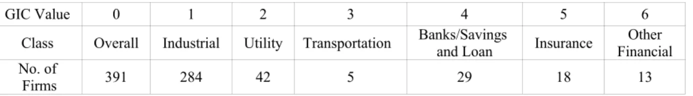
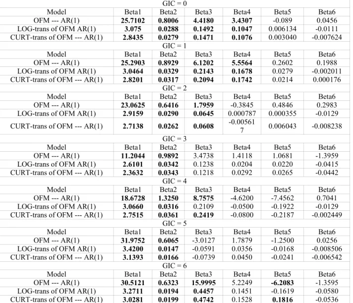
After using PROC AUTOREG to the data in each GIC group (see Table 1.3.3 for the General Industrial Classification Distribution), the estimated regression coefficients for three models are collected in Table 1.3.4. The results show that the intercept, BPS and abnormal earnings per share of the first two following quarters are generally significant in the Ohlson Model. (The values in bold are significant, others are insignificant.)

Table 1.3.3 --- General Industrial Classification (GIC) Distribution

GIC Value 0 1 2 3 4 5 6

Class Overall Industrial Utility Transportation Banks/Savings _{and Loan} Insurance _FinancialOther No. of

Firms 391 284 42 5 29 18 13

(13)

The PROC AUTOREG procedure also gives the predicted values of the 21st_{period using}

the base data. To compare the predictive abilities among the three selected models for different GIC groups, the criterion is defined as

R=(yˆ21 −y21)/y21 (1.3.1)

where R is the relative difference of predicted stock price over real stock price for a company, yˆ₂₁ is the predicted stock price of a company for the 21st_period,

21

y is the real stock price of a company for the 21st_period.

Table 1.3.4 --- Estimated Parameters from Base Data

GIC = 0

Model Beta1 Beta2 Beta3 Beta4 Beta5 Beta6

OFM --- AR(1) 25.7102 0.8006 4.4180 3.4307 -0.089 0.0456

LOG-trans of OFM AR(1) 3.075 0.0288 0.1492 0.1047 0.006134 -0.0111

CURT-trans of OFM --- AR(1) 2.8435 0.0279 0.1471 0.1076 0.003040 -0.007624

GIC = 1

OFM --- AR(1) 25.2903 0.8929 6.1202 5.5564 0.2602 0.1988

LOG-trans of OFM AR(1) 3.0464 0.0329 0.2143 0.1678 0.0279 -0.002011

CURT-trans of OFM --- AR(1) 2.8201 0.0317 0.2094 0.1742 0.0214 0.000176

GIC = 2

OFM --- AR(1) 23.0625 0.6416 1.7959 -0.3845 0.4846 0.2983

LOG-trans of OFM AR(1) 2.9159 0.0290 0.0645 0.000787 0.000355 -0.0129

CURT-trans of OFM --- AR(1) 2.7138 0.0262 0.0608 -0.00561₇ 0.006043 -0.008238

GIC = 3

OFM --- AR(1) 11.2044 0.9892 3.4738 1.4118 1.0681 -1.3959

LOG-trans of OFM AR(1) 2.6101 0.0342 0.1238 0.0204 0.0220 -0.0415

CURT-trans of OFM --- AR(1) 2.3632 0.0343 0.1218 0.0292 0.0265 -0.0442

GIC = 4

OFM --- AR(1) 18.6728 1.3250 8.7575 -4.6200 -7.4562 0.7041

LOG-trans of OFM AR(1) 3.0660 0.0316 0.2109 -0.0500 -0.1922 -0.0129

CURT-trans of OFM --- AR(1) 2.7515 0.0361 0.2419 -0.0800 -0.2187 -0.002449

GIC = 5

OFM --- AR(1) 31.9752 0.6065 -3.0127 1.7879 -1.2500 0.0256

LOG-trans of OFM AR(1) 3.4200 0.0147 -0.0591 0.0356 -0.0168 -0.008506

CURT-trans of OFM --- AR(1) 3.1393 0.0166 -0.0739 0.0450 -0.0241 -0.006542

GIC = 6

OFM --- AR(1) 30.5121 0.6323 15.9995 5.2249 -6.2083 -1.3595

LOG-trans of OFM AR(1) 3.2711 0.0194 0.4457 0.1451 -0.1619 -0.0580

(14)

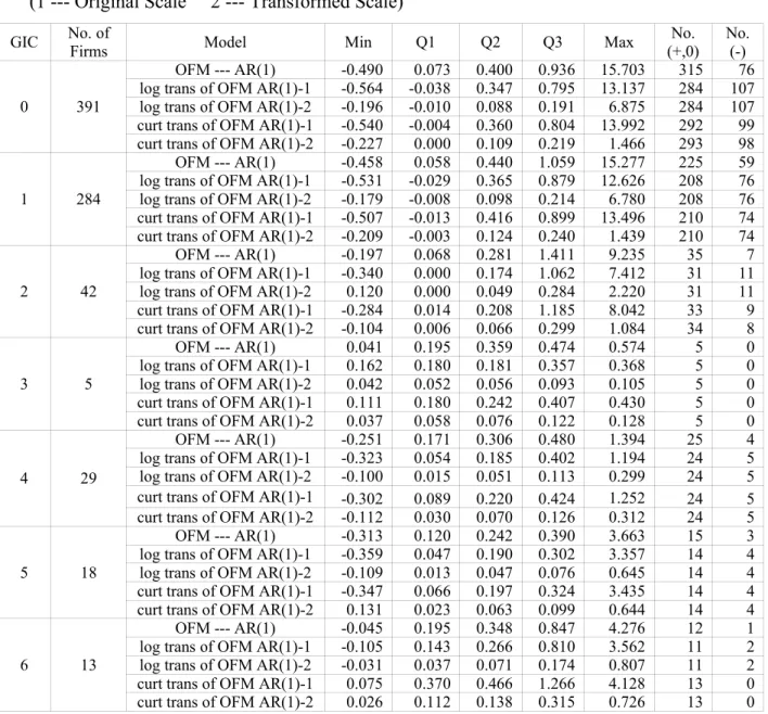
The following conclusions can be drawn from Table 1.3.5 where the quantiles of R, the number of nonnegative R’s (No.(+,0)) and the number of negative R’s (No. (-)) are collected. The digital “1” and “2” after the names of transformations are to distinguish different scales of measurement. “1” denotes using the original scale, “2” denotes using the transformed scale.

Table 1.3.5 --- Quantiles of R and Number of Nonnegative/Negative R’s (1 --- Original Scale 2 --- Transformed Scale)

GIC No. of_Firms Model Min Q1 Q2 Q3 Max _(+,0)No. No._(-)

0 391

OFM --- AR(1) -0.490 0.073 0.400 0.936 15.703 315 76

log trans of OFM AR(1)-1 -0.564 -0.038 0.347 0.795 13.137 284 107

curt trans of OFM AR(1)-1 -0.540 -0.004 0.360 0.804 13.992 292 99

curt trans of OFM AR(1)-2 -0.227 0.000 0.109 0.219 1.466 293 98

1 284

OFM --- AR(1) -0.458 0.058 0.440 1.059 15.277 225 59

2 42

OFM --- AR(1) -0.197 0.068 0.281 1.411 9.235 35 7

log trans of OFM AR(1)-1 -0.340 0.000 0.174 1.062 7.412 31 11

log trans of OFM AR(1)-2 0.120 0.000 0.049 0.284 2.220 31 11

3 5

OFM --- AR(1) 0.041 0.195 0.359 0.474 0.574 5 0

curt trans of OFM AR(1)-1 0.111 0.180 0.242 0.407 0.430 5 0

4 29

OFM --- AR(1) -0.251 0.171 0.306 0.480 1.394 25 4

5 18

OFM --- AR(1) -0.313 0.120 0.242 0.390 3.663 15 3

6 13

OFM --- AR(1) -0.045 0.195 0.348 0.847 4.276 12 1

(15)

The empirical results show that the distributions of Rare asymmetrical with long tails, which suggests the 50% quantile (Q2) of R as a major criterion. From Table 1.3.5, the following conclusions can be drawn.

• Based on Q2 values in original scale, the ratio value ranges from 24.2% (GIC = 5) to 44% (GIC = 1) and 40% overall (GIC = 0) under no transformation, from 17.4% (GIC = 2) to 36.5% (GIC = 1) and 34.7% overall (GIC = 0) under log transformation, and from 19.7% (GIC = 5) to 46.6% (GIC = 6) and 36% overall (GIC = 0) under cubic root transformation. Based on Q2 values in transformed scale, the ratio value ranges from 4.7% (GIC = 5) to 9.8% (GIC = 1) and 8.8% overall (GIC = 0) under log transformation, and from 6.3% (GIC = 5) to 13.8% (GIC = 6) and 10.9% overall (GIC = 0) under cubic root transformation. These conclude that the log transformation improves the predictive ability more than the cubic root transformation does while using the classical method.

• In all cases, the number nonnegativeR’s is much larger than the number of negativeR’s, which shows the high overestimation by the classical method.

The too large magnitude of Rand the extremely high overestimation state that using the classical method (the PROC AUTOREG procedure) to interpret the Ohlson model is not efficient enough in forecasting stock prices. A better approach is desired to improve both the estimative and predictive abilities of the Ohlson model.

Summarily, the exploratory data analysis by PROC REG/AUTOREG confirms the AR(1) assumption of the innovation term in the Ohlson model, and the promising effect of adopting logarithmic transformation as well as cubic root transformation. It suggests that the remaining work focus on 3 models: OFM --- AR(1), log trans of OFM AR(1) and curt trans of OFM --- AR(1). Since the Ohlson model is not able to predict the stock price efficiently by the classical means, this paper applies an innovative statistical method, Bayesian statistical analysis, to the 3 chosen models in the remaining work.

1.4 An Outline of Bayesian Statistical Analysis

In the following three chapters of this paper, Bayesian approaches are used for the purpose of satisfying the requirement of improving both the estimative and predictive

(16)

qualities of the Ohlson model, comparing to the classical methods. In detail, Chapter 2 uses the most basic Bayesian techniques to each company, which is the case that different companies have different regression coefficients; Chapter 3 applies the Bayesian method by letting all the companies in each group share the same regression coefficients. While Chapter 2 represents the individual analysis, Chapter 3 represents the grouping analysis. And Chapter 4 ends up to be the adaptive analysis by pooling information across

companies. That is, different companies have different regression coefficients in Chapter 4, and in the mean time they are pooled together. Basically, Chapter 4 compromises the ideas in Chapter 2 and the ones in Chapter 3.

For each Bayesian approach in following three chapters, the main tasks are to make inferences for the regression coefficients (or parameters), evaluate the model adequacy and test the predictive ability of the Ohlson model. Chapter 5 concludes all the work in this paper, which includes the comparison among the three Bayesian approaches as well as the comparison of the best Bayesian approach to the classical method.

(17)

Chapter 2

Bayesian Statistical Analysis for Individual Firm

2.1 Bayesian Version of the Ohlson Model for a Single Firm

As an extreme case, this chapter assumes all the companies are independent of each other and have their own regression coefficients in the Ohlson model. At the very beginning of applying the Bayesian statistical analysis to each company, a Bayesian version of the Ohlson model is set up in the following three steps.

First, for a specific company, describe the observation ( 1, 2, , )

~ T y y y y=  _{by the} parameters{ , , , 2} ~ µ ρ σ

β _{. Under the assumption that the observations are conditionally} independent among the time periods, we can get the likelihood function from expression (1.1.5):

∏

= − −     ₋ + ⋅ + = T t t t t t x y x y N x y N y p 2 2 ~ ' 1 ~ 1 ~ ' ~ 2 ~ ' 1 ~ 1 2 ~ ~ ) , | ( ) , | ( ) , , , | ( β µ ρσ β µ σ β ρ β σ . (2.1.1)

Second, assign a prior distribution to each unknown parameter. The prior distribution represents a population of possible parameter values, from which the parameter of current interest has been drawn. The guiding principle is to express the knowledge (and

uncertainty) about the parameter as if its value could be thought of as a random realization from the prior distribution. In order to get the practical advantage of being interpretable as additional data and computational convenience, this paper assigns the conjugate prior distributions as follows:

). , | ( ) ( ), 1 , 1 | ( ) ( ), , | ( ) ( ), , | ( ) ( 2 2 2 0 0 0 0 ~ ~ ~ b a I U N N_K σ σ π ρ ρ π σ µ µ µ π θ β β π Γ = − = = ∆ = (2.1.2)

(18)

The hyperparameters { , 0, 0, 02} 0

~ µ σ

θ ∆ _{in (2.1.2) are set as follows.}

(P2.1) ~ 1 0 ~ B (X'X) X'y − = = θ _.

The idea of setting θ_~₀ is to use the estimation of

~

β_{in the ordinary linear} regression model , , , 1 ), , 0 ( ~ , 2 ~ ' _N _t _T x y_t = _tβ+ε_t ε_tiid σ =  (OLM-1)

by the method of least squares. Note that

(

'

)

~ ' 2 ~ ' 1 ~ ,x , ,xT x

X =  _{is the matrix of all}

covariates together with an intercept, (1, , 1, 2, 3, 4)' ' ~ a t a t a t a t t t bv x x x x x = ₊ ₊ ₊ ₊ ₍t =1 , ,T ) is the regression coefficient vector consisting of the 1 and predictors, andT is the number of time periods.

(P2.2) P T SS X X E − = ∆ −1

0 100( ' ) , whereSSE = y'y−B'X'y is the sum of squares of the errors of (OLM-1), P is the number of regression coefficients (including the intercept),

P T

SS_E

− is the estimation of the σ2 in (OLM-1) by the method of least squares, and P T SS X X E − −1 ) '

( is the estimation of the covariance matrix of β_~ in (OLM-1). Multiplying the estimation of the covariance matrix by 100 is to add more variability. (P2.3) ( ) 1 ~ 1 0

∑

= − ₋ = T i i i x B y T µ . From 1, 1 ~ (0, 2) ~ ' 1 1 x β µ ε ε N σ

y = + + _{in expression (1.1.5), we can get the}

estimation of µ which is y x'B

1 1

ˆ = −

µ . Taking each observation can as starting point, that is,

T i N x y_i _i _i, _i ~ (0, 2), 1,2, , ~ ' ₊ ₌ _ − = β ε ε σ µ . (OLM-2)

The idea of setting µ0is to use the averaged estimation of µ in (OLM-2).

(P2.4) P T SSE − = 2 0

(19)

squares. (P2.5) a=b=0.001.

These two hyperparameters are chosen by convention or experience in Bayesian statistical analysis.

Assume that all the parameters are independent of each other, the joint prior distribution of the parameters can be expressed as

( , , , ) ( | , 0) ( | 0, 02) ( | 1,1), ( 2 | , ). 0 ~ ~ 2 ~ N N U I a b p β µ ρ σ = _K β θ ∆ ⋅ µ µ σ ⋅ ρ − ⋅Γ σ _(2.1.3)

Finally, from the likelihood function in (2.1.1) and joint prior distribution in (2.1.3), we can get the posterior distribution of the parameters given the data using Bayes’ rule:

. ) , | ( ) , | ( ) , | ( ), 1 , 1 | ( ) , | ( ) , | ( ) , , , | ( ) , , , ( ) | , , , ( 2 2 ~ ' 1 ~ 1 ~ ' ~ 2 ~ ' 1 ~ 1 2 2 0 0 0 0 ~ ~ 2 ~ ~ 2 ~ ~ 2 ~

∏

= − −     ₋ + ⋅ + ⋅ Γ ⋅ − ⋅ ⋅ ∆ ∝ ∝ T t t t t t K x y x y N x y N b a I U N N y p p y p σ β ρ β σ µ β σ ρ σ µ µ θ β σ ρ µ β σ ρ µ β σ ρ µ β (2.1.4) 2.2 Gibbs Sampling

The Gibbs sampler is an iterative Monte Carlo algorithm designed to extract the posterior distribution from the tractable complete conditional distributions rather than directly from the intractable joint posterior distribution, which is difficult to acquire in explicit form. In this chapter, the target is to make inferences on the parameters { , , , 2}

~ µ ρ σ

β _{given the}

data. We consider the complete conditional distributions ( |.)

~ β π _,_π₍_µ_|_.)_,_π₍_ρ_|_.)_{, and} .) | (_σ2

π respectively. Here, the conditioning argument “⋅” denotes the observation and the remaining parameters. From the posterior distribution in (2.1.4) we can derive the complete conditional distributions.

(20)

First,       ₋_Λ ₊_Λ _ΛΣ β β µ θ σ ρ µ β | , , , ~ ( ) , ~ ~ 2 ~ ~ I N y _K , where

(

)(

)

(

)

_   ₋ ₋ ₋ ₋     ₊ ₋ ₋ =

∑

= − − − = − − T t t t t t T t t t t t x x y y x y x x x x x x 2 ' 1 ~ ~ 1 ' 1 ~ 1 1 2 ' 1 ~ ~ 1 ~ ~ ' 1 ~ 1 ~ ~ ρ ρ ( µ) 2( ρ ) ρ µ β ,

(

)(

)

∑

= − − − − + = Σ T t t t t t x x x x x x 2 ' 1 ~ ~ 1 ~ ~ ' 1 ~ 1 ~ ρ ρ β , 1 1 1 1 1 1 1 1 1 1 1 ₎ ₍ ₎ ₍ ₎ ₍ ₎ (∆− +Σ− − Σ− = Σ ∆− +Σ Σ− − = Σ ∆− +∆∆− − =∆ Σ +∆ − = Λ _β _β _β _β _β _β _β . Second,       _Φ     − Φ + Φ − 2 ~ ' 1 ~ 1 0 2 ~ ~, , , ~ (1 ) , | β ρ σ µ β σ µ y N y x , where ₂ ₂. 0 2 0 σ σ σ + = Φ Third,                 −     −     ₋     − −

∑

− = − = − = + + 1 1 2 ~ ' ~ 2 1 1 2 ~ ' ~ 1 1 ~ ' 1 ~ 1 ~ ' ~ 2 ~ ~ , ) 1 , 1 ( ~ , , , | _T t t t T t t t T t t t t t x y x y x y x y N U y β σ β β β σ µ β ρ . Fourth, . 2 , 2 ~ , , , | 2 2 ~ ' 1 ~ 1 ~ ' ~ 2 ~ ' 1 ~ 1 ~ ~ 2                       ₋ − − +     ₋ ₋ + + −

∑

= − − T t t t t t x y x y x y b T a gamma Inv y β ρ β µ β ρ µ β σ

The Gibbs sampler is implemented using the following six steps. Step 1, obtain starting values { 0, 0, 0, 2,0}

~ ρ µ σ β _. Step 2, draw t ~ β _from ( | , , , ) ~ 1 , 2 1 1 ~ y t t t− _ρ − _σ − µ β π _.

Step 3, draw _µt_from ( | , , , )

~ 1 , 2 1 ~ y t t t _ρ − _σ − β µ π _.

Step 4, draw _ρt_from ( | , , , )

~ 1 , 2 ~ y t t t _µ _σ − β ρ π _.

Step 5, draw _σ2,t_from ( | , , , )

~ ~

2 _βt _µt _ρt _y

σ

π _.

(21)

This paper chooses the starting points { 0, 0, 0, 2,0} ~ ρ µ σ β _{as follows.} First, ~ 1 0 ~ ' ) ' (X X − X y = β _. Second, , ( _~ 1)( 1 _~ ₁ 2) 1 1 12 22 11 12 0 _SS _y _x _B _ave _y _x _B _ave SS SS SS t t t T t t − − − − = = + + − =

∑

ρ , where . 1 ) ( 2 , 1 ) ( 1 and , ) 2 ( , ) 1 ( ~ 2 ~ 1 1 2 ~ 2 22 2 ~ 1 1 11 − − = − − = − − = − − =

∑

= − = = − = T B x y ave T B x y ave ave B x y SS ave B x y SS t T t t t T t t t T t t t T t t Third, ( ) 1 ~ 1 0

∑

= − ₋ = T i i i x B y T µ . Fourth, p T SS_E − = 0 , 2 σ .

The ideas of setting _β0_,_µ0_and_σ2,0_{are the same as the ones of setting the}

hyper-parameters { , 0, 0, 02} 0

~ µ σ

θ ∆ _{in (2.1.2), which is using the estimation of parameters from} the (OLM-1) and (OLM-2). The idea of setting _ρ0_{is taking it as the autocorrelation of}

time series t t t t t y x v v = − β =ρ ₋₁+ε ~ ' ~ in an AR(1) structure.

This chapter develops two algorithms using Markov-chain Monte Carlo methods, a restricted algorithm that enforces stationarity condition by letting |ρ|<1 on the series and an unrestricted algorithm that does not.

2.3 Forecast

After getting the posterior distribution of the parameters, we can use it to predict the future stock prices. In this paper we wish to forecast the stock price at time period T + 1

(22)

denoted by yT+1, given the data y(T) =(y1,y2,,yT). Letting { , , , } 2 ~ µ ρ σ β = Ω _{, the}

prediction can be sampled from the posterior predictive distribution

f(y_T₊₁|y₍_T₎)=

∫

f(y_T₊₁,Ω|y)π(Ω|y)dΩ. (2.3.1) Letting _Ω(1)_,_Ω(2)_,__,_Ω(M)_{be a sequence of range M from the Gibbs sampler, an}

estimator of f(y_T₊₁|y₍_T₎) is

∑

= + − + = Ω M h T h T T T y M f y y y f 1 ) ( ) ( 1 1 ) ( 1| ) ( | , ) ( ˆ _{. (2.3.2)}

To get samples of yT+1, we use data argumentation to fill inyT+1 to each Ω(h),

M

h=1 ,2 , , , to get ( ) 1

h T

y ₊ , h=1 ,2 , ,M , from the normal distribution in (2.3.3). | , ~ ( ( ), 2). ~ ' ~ ~ ' 1 ~ ) ( 1 β ρ β σ T T T T T y N x y x y Ω + − + + (2.3.3)

The 95% predictive credible interval for y_T₊₁ can be computed from the 2.5% and 97.5% empirical quantiles of the values ( )

1

h T

y ₊ , h=1 ,2 , ,M.

2.4 Conditional Predictive Ordinate

We want to assess the goodness of fit of the Ohlson Model to the data. One procedure is to calculate the log conditional predictive ordinatelog(p(y_t₊₁| y₍_t₎)) with

( | ) ( | , ), 1 () ) ( 1 ) ( ) ( 1

∑

= + + ≈ Ω M h t h t h t t t y p y y y p ϖ (2.4.1)

whereyt+1 denotes the random future observation at period t + 1,

) , , , ( ₁ ₂ ) (t y y yt

y =  denotes the observations from period 1 to t, _Ω(h)_{denotes the h}th_draw

of the parameters from the Gibbs sampler, and

. , , 1 , ) | ( ) | ( ) | ( ) | ( 1 ( ) ) ( ) ( ) ( ) ( ) ( ) ( _h _M y f y f y f y f M k h h t h h t h t =  Ω Ω Ω Ω =

∑

= ϖ

(23)

2.5 Empirical Results of Individual Bayesian Analysis

After getting the Bayesian version of the Ohlson model for each firm, we fit it to the data corresponding to each company in the base data set. 11000 iterations are run in the Gibbs sampler, the first 1000 draws are thrown away, and finally 1000 draws are collected by picking one draw every 10 paces. Since there are too many companies (391), the results are averaged for each GIC group. Besides making conclusions from the empirical results, this chapter also tries to decide which models from {OFM --- AR(1), log trans of OFM AR(1), curt trans of OFM AR(1)} will be used for further Bayesian analysis, whether the stationary restriction is needed and which measurement scale to use, original one or the transformed one.

Four criteria are used for the model valuation: the relative difference of the predicted stock price over the real stock price (R), numbers of nonnegative ratios and negative ratios (No.(+,0) and No.(-,0)), length of 95% credible intervals, and log conditional predictive ordinate (CPO). The ratio of residual is defined in the same way as (1.3.1) in Chapter 1. But in this chapter and the following two chapters, No.(+,0) and No.(-,0) denote the rounded numbers of nonnegative and negative ratios divided by 1000 respectively.

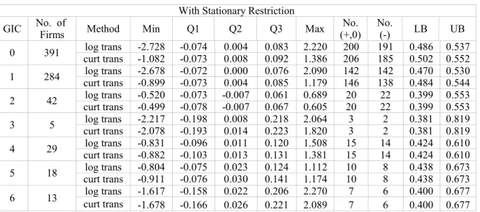
The quantiles of R as well as No.(+,0) and No.(-,0) are collected in Table 2.5.1(a) while using the stationary restriction, and in Table 2.5.1 (b) for the case without the stationary restriction.

The LB and UB in these two tables are calculated from No.(+,0) and No.(-,0) by formulas: , / ) ˆ 1 ( ˆ ˆ , / ) ˆ 1 ( ˆ ˆ p p N UB p p p N p LB= − − = + − where pˆ =No.(+,0)/N, ). .( ) 0 , .(+ + − = No No

N They are the lower bound (LB) and upper bound (UB) of the 95% confidence interval of pˆ which are used to check the state of overestimation. If 0.5 is between LB and UB, then the method does not overestimate the stock prices, and vice versa.

(24)

Table 2.5.1(a) --- With Stationary Restriction (1-Original Scale, 2-Transformed Scale)

GIC No. of_Firms Method Min Q1 Q2 Q3 Max _(+,0)No. No._(-) LB UB

0 391 no trans -25.141 -0.109 0.070 0.289 19.290 236 155 0.579 0.628 log trans-1 -0.963 -0.101 0.069 0.274 23.080 237 154 0.581 0.631 log trans-2 -7.275 -0.032 0.020 0.075 3.094 237 154 0.581 0.631 curt trans-1 -1.094 -0.105 0.065 0.269 14.541 235 156 0.576 0.626 curt trans-2 -1.455 -0.035 0.022 0.084 1.497 237 154 0.581 0.631 1 284 no trans -25.141 -0.114 0.077 0.308 19.290 172 112 0.577 0.635 log trans-1 -0.963 -0.105 0.075 0.289 23.080 173 111 0.580 0.638 log trans-2 -7.275 -0.034 0.022 0.079 3.094 173 111 0.580 0.638 curt trans-1 -1.094 -0.110 0.071 0.285 1.493 171 113 0.573 0.631 curt trans-2 -1.455 -0.037 0.024 0.088 1.497 173 111 0.580 0.638 2 42 no trans -12.948 -0.152 0.027 0.237 12.170 23 19 0.471 0.624 log trans-1 -0.938 -0.147 0.017 0.211 15.154 22 20 0.447 0.601 log trans-2 -2.891 -0.048 0.005 0.061 2.226 22 20 0.447 0.601 curt trans-1 -1.018 -0.150 0.017 0.211 11.854 22 20 0.447 0.601 curt trans-2 -1.264 -0.052 0.007 0.067 1.344 22 20 0.447 0.601 3 5 no trans -1.292 -0.025 0.089 0.215 1.239 4 1 0.621 0.979 log trans-1 -0.652 -0.042 0.072 0.207 2.099 3 2 0.381 0.819 log trans-2 -0.315 -0.013 0.021 0.058 0.425 3 2 0.381 0.819 curt trans-1 -0.752 -0.040 0.073 0.206 1.653 3 2 0.381 0.819 curt trans-2 -0.371 -0.013 0.025 0.067 0.386 3 2 0.381 0.819 4 29 no trans -2.004 -0.050 0.080 0.243 2.156 19 10 0.567 0.743 log trans-1 -0.950 -0.043 0.088 0.251 4.336 19 10 0.567 0.743 log trans-2 -0.754 -0.013 0.025 0.066 0.485 19 10 0.567 0.743 curt trans-1 -0.897 -0.049 0.081 0.241 3.118 19 10 0.567 0.743 curt trans-2 -0.531 -0.015 0.028 0.076 0.605 19 10 0.567 0.743 5 18 no trans -1.587 -0.061 0.090 0.278 4.695 12 6 0.556 0.778 log trans-1 -0.089 -0.048 0.089 0.272 5.143 12 6 0.556 0.778 log trans-2 -0.437 -0.014 0.024 0.067 0.795 12 6 0.556 0.778 curt trans-1 -0.759 -0.053 0.086 0.270 4.862 12 6 0.556 0.778 curt trans-2 -0.377 -0.017 0.029 0.084 0.804 12 6 0.556 0.778 6 13 no trans -8.584 -0.139 0.025 0.244 7.027 7 6 0.400 0.677 log trans-1 -0.810 -0.119 0.037 0.222 5.635 7 6 0.400 0.677 log trans-2 -0.882 -0.036 0.011 0.061 0.957 7 6 0.400 0.677 curt trans-1 -0.994 -0.126 0.032 0.219 4.961 7 6 0.400 0.677 curt trans-2 -0.818 -0.043 0.012 0.069 0.814 7 6 0.400 0.677

(25)

Table 2.5.1(b) --- Without Stationary Restriction (1-Original Scale, 2-Transformed Scale)

GIC No. of_Firms Method Min Q1 Q2 Q3 Max _(+,0)No. No._(-) LB UB

0 391 no trans -26.845 -0.124 0.060 0.273 16.443 230 161 0.563 0.613 log trans-1 -0.987 -0.113 0.059 0.260 43.221 231 160 0.566 0.616 log trans-2 -5.938 -0.036 0.017 0.071 2.744 231 160 0.566 0.616 curt trans-1 -1.834 -0.119 0.054 0.255 16.583 228 163 0.558 0.608 curt trans-2 -1.942 -0.040 0.019 0.080 1.602 230 161 0.563 0.613 1 284 no trans -26.715 -0.120 0.060 0.263 17.286 168 116 0.562 0.621 log trans-1 -0.975 -0.107 0.063 0.259 33.557 170 114 0.570 0.628 log trans-2 -5.938 -0.038 0.019 0.075 2.744 169 115 0.566 0.624 curt trans-1 -1.834 -0.122 0.060 0.269 15.583 167 117 0.559 0.617 curt trans-2 -1.942 -0.042 0.021 0.084 1.602 168 116 0.562 0.621 2 42 no trans -4.539 -0.121 0.052 0.245 4.784 24 18 0.495 0.648 log trans-1 -0.862 -0.111 0.061 0.264 9.311 25 17 0.519 0.671 log trans-2 -3.640 -0.053 0.002 0.057 1.956 21 21 0.423 0.577 curt trans-1 -1.039 -0.165 0.005 0.198 9.244 21 21 0.423 0.577 curt trans-2 -1.339 -0.057 0.003 0.063 1.173 22 19 0.459 0.614 3 5 no trans -16.924 -0.374 0.038 0.390 64.950 3 2 0.381 0.819 log trans-1 -0.998 -0.199 0.035 0.280 58.857 3 2 0.381 0.819 log trans-2 -0.266 -0.167 0.019 0.054 0.507 3 2 0.381 0.819 curt trans-1 -0.638 -0.052 0.066 0.193 2.071 3 2 0.381 0.819 curt trans-2 -0.286 -0.016 0.023 0.062 0.455 3 2 0.381 0.819 4 29 no trans -4.497 -0.097 -0.085 0.313 4.389 18 11 0.531 0.711 log trans-1 -0.860 -0.098 0.080 0.303 9.166 18 11 0.531 0.711 log trans-2 -0.467 -0.016 0.024 0.067 0.795 19 10 0.567 0.743 curt trans-1 -0.907 -0.057 0.078 0.238 2.799 19 10 0.567 0.743 curt trans-2 -0.546 -0.018 0.026 0.075 0.562 19 10 0.567 0.743 5 18 no trans -4.912 -0.137 0.083 0.322 4.025 11 7 0.496 0.726 log trans-1 -0.994 -0.111 0.077 0.299 10.331 11 7 0.496 0.726 log trans-2 -0.387 -0.018 0.021 0.065 0.631 12 6 0.556 0.778 curt trans-1 -0.836 -0.069 0.074 0.258 3.297 11 7 0.496 0.726 curt trans-2 -0.452 -0.022 0.025 0.081 0.627 11 7 0.496 0.726 6 13 no trans -5.892 -0.199 0.044 0.286 4.361 7 6 0.400 0.677 log trans-1 -0.851 -0.152 0.044 0.260 9.485 7 6 0.400 0.677 log trans-2 -0.774 -0.047 0.003 0.056 0.773 7 6 0.400 0.677 curt trans-1 -0.938 -0.164 0.001 0.192 3.719 7 6 0.400 0.677 curt trans-2 -0.605 -0.057 0.002 0.062 0.678 7 6 0.400 0.677

Similar to Chapter 1, the empirical results show that the distributions of Rare asymmetrical with long tails. This chapter also uses the 50% quantile (Q2) of R as a major criterion. The following conclusions can be drawn from Table 2.5.1(a).

• Based on Q2 values in original scale, the ratio value ranges from 2.5% (GIC = 6) to 9% (GIC = 5) and 7% overall (GIC = 0) under no transformation, from 1.7% (GIC = 2) to 8.9% (GIC = 5) and 6.9% overall (GIC = 0) under log

transformation, and from 1.7% (GIC = 2) to 8.6% (GIC = 5) and 6.5% overall (GIC = 0) under cubic root transformation. Based on Q2 values in transformed

(26)

scale, the ratio value ranges from 0.5% (GIC = 2) to 2.5% (GIC = 4) and 2% overall (GIC = 0) under log transformation, and from 0.7% (GIC = 2) to 2.9% (GIC = 5) and 2.2% overall (GIC = 0) under cubic root transformation. These conclude that with stationary restriction, both the log transformation and the cubic root transformation improve the predictive ability comparing to the method without using any transformation

• When GIC is 0, 1, or 4, 0.5 is not between LB and UB; when GIC is 3 or 6, 0.5 is not between LB and UB; when GIC is 2, 0.5 is between LB and UB except in the case of using log transformation under the original scale; when GIC is 5, 0.5 is between LB and UB except in the case of using log transformation under the transformed scale. Since 0.5 is not between LB and UB for large groups, we conclude that using Bayesian method to each company by restricting stationarity overestimates the stock prices.

Table 2.5.1(b) gives the following conclusions.

• Based on Q2 values in original scale, the ratio value ranges from 3.8% (GIC = 3) to -8.5% (GIC = 4) and 6% overall (GIC = 0) under no transformation, from 3.5% (GIC = 3) to 8% (GIC = 4) and 5.9% overall (GIC = 0) under log transformation, and from 0.1% (GIC = 6) to 7.8% (GIC = 4) and 5.4% overall (GIC = 0) under cubic root transformation. Based on Q2 values in transformed scale, the ratio value ranges from 0.2% (GIC = 2) to 2.4% (GIC = 4) and 1.7% overall (GIC = 0) under log transformation, and from 0.2% (GIC = 6) to 2.6% (GIC = 4) and 1.9% overall (GIC = 0) under cubic root transformation. These conclude that both the log transformation and the cubic root transformation also improve the predictive ability comparing to the method without using any transformation without stationary restriction.

• When GIC is 0, 1, or 4, 0.5 is not between LB and UB; when GIC is 3 or 6, 0.5 is not between LB and UB; when GIC is 2, 0.5 is between LB and UB except in the case of using log transformation under the original scale; when GIC is 5, 0.5 is between LB and UB except in the case of using log transformation under the transformed scale. Since 0.5 is not between LB and UB for large groups, we

(27)

conclude that using Bayesian method to each company by restricting stationarity overestimates the stock prices.

Comparing the conclusions from Table 2.5.1(a) to the ones from Table 2.5.1(b), there exist some slight differences between them, but this paper considers that those differences are minor. There are two things in common. First, using both transformations can

enhance the predictive ability. Second, the Bayesian approach to each company overestimates the stock prices for most companies.

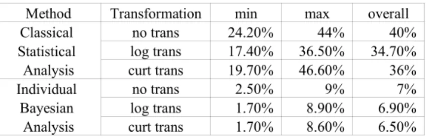
Table 2.5.2 --- Min, Max and Overall Values of R

Method Transformation min max overall

Classical no trans 24.20% 44% 40%

Statistical log trans 17.40% 36.50% 34.70%

Analysis curt trans 19.70% 46.60% 36%

Individual no trans 2.50% 9% 7%

Bayesian log trans 1.70% 8.90% 6.90%

Analysis curt trans 1.70% 8.60% 6.50%

This paper uses the minimum, maximum and overall values of R to compare the

Bayesian approaches with the classical method. Table 2.5.2 gives those values under the original scale from both classical statistical analysis and individual Bayesian analysis. It shows the huge improvement of using individual Bayesian approach to the Ohlson model, compared to the classical method.

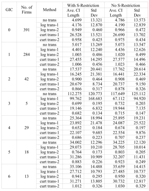
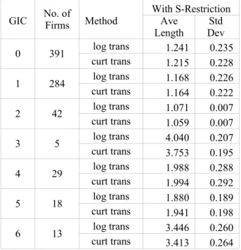
The average lengths of credible interval (CI) are in Table 2.5.3, from which it is easy to see that they are shorter under stationary restriction than without stationary restriction. In all case, GIC 3 has the longest length, GIC 0 and 1 have the shortest length. GIC 2, 4, 5 6 have similar length. It seems that the more companies a GIC group has, the shorter the CI is. This hints that pooling information across companies may improve the predictive ability of the Ohlson model. Generally, the average lengths of CI’s are quite wide under the original scale, and extremely smaller under the transformed scale. The standard deviations are very big under the original scale and much smaller under the transformed scale. This implies that the results under the transformed scale make more sense, which can also been indicated by Table 2.5.1(a) and (b).

(28)

Table 2.5.3 --- Average Length of Credible Interval

GIC No. of_Firms Method Ave. CIWith S-Restriction No S-Restriction Length DevStd Ave. CILength Std Dev

0 391 no trans 4.699 13.321 4.786 13.573 log trans-1 4.176 12.870 4.190 12.839 log trans-2 0.949 0.460 0.966 0.472 curt trans-1 26.528 13.521 26.690 13.702 curt trans-2 0.958 0.425 0.975 0.434 1 284 no trans 5.017 13.269 5.073 13.547 log trans-1 4.401 12.240 4.436 12.626 log trans-2 1.003 0.486 1.020 0.499 curt trans-1 27.455 14.295 27.577 14.496 curt trans-2 1.006 0.456 1.023 0.466 2 42 no trans 17.537 20.441 17.762 20.614 log trans-1 16.245 21.381 16.441 22.334 log trans-2 0.900 0.464 0.908 0.469 curt trans-1 20.679 8.734 20.737 9.150 curt trans-2 0.866 0.317 0.878 0.326 3 5 no trans 112.275 120.773 117.649 125.112 log trans-1 99.762 168.683 67.112 94.920 log trans-2 0.699 0.195 0.732 0.203 curt trans-1 19.146 6.832 19.944 7.135 curt trans-2 0.682 0.134 0.715 0.147 4 29 no trans 25.364 18.994 25.895 19.231 log trans-1 23.892 21.478 24.087 25.522 log trans-2 0.652 0.184 0.674 0.197 curt trans-1 22.107 9.685 22.554 9.876 curt trans-2 0.686 0.223 0.707 0.237 5 18 no trans 34.002 12.296 34.225 12.120 log trans-1 29.073 10.210 28.705 10.014 log trans-2 0.764 0.173 0.803 0.205 curt trans-1 31.286 10.909 32.207 11.431 curt trans-2 0.883 0.226 0.923 0.249 6 13 no trans 35.106 14.488 35.659 14.415 log trans-1 27.712 10.793 27.485 10.737 log trans-2 0.941 0.295 0.950 0.320 curt trans-1 31.271 13.805 30.732 12.817 curt trans-2 1.012 0.326 1.030 0.329

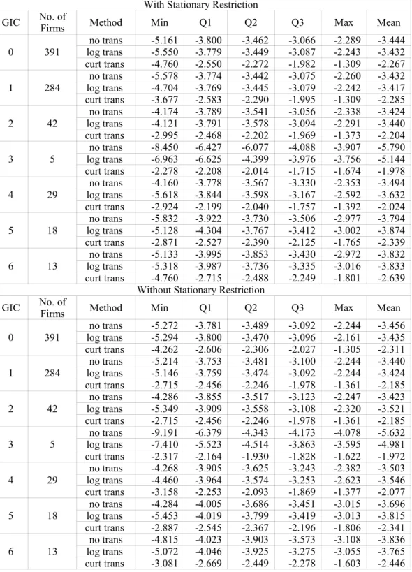
The log conditional predictive ordinate (CPO) is to evaluate the model fitting adequacy. It always has negative values and is calculated under the original scale in this chapter. The bigger CPO is, the better the model fits the data.

Table 2.5.4 gives the quantiles and mean of CPO in each case and shows that the CPO values are smaller under stationary restriction than without stationary restriction.

(29)

Table 2.5.4 --- CPO

With Stationary Restriction

GIC No. of_Firms Method Min Q1 Q2 Q3 Max Mean

0 391 log trans no trans -5.161-5.550 -3.800-3.779 -3.462-3.449 -3.066-3.087 -2.289-2.243 -3.444-3.432

curt trans -4.760 -2.550 -2.272 -1.982 -1.309 -2.267

curt trans -3.677 -2.583 -2.290 -1.995 -1.309 -2.285

curt trans -2.995 -2.468 -2.202 -1.969 -1.373 -2.204

curt trans -2.278 -2.208 -2.014 -1.715 -1.674 -1.978

curt trans -2.924 -2.199 -2.040 -1.757 -1.392 -2.024

curt trans -2.871 -2.527 -2.390 -2.125 -1.765 -2.339

curt trans -4.760 -2.715 -2.488 -2.249 -1.801 -2.639

Without Stationary Restriction

GIC No. of_Firms Method Min Q1 Q2 Q3 Max Mean

curt trans -4.262 -2.606 -2.306 -2.027 -1.305 -2.311

curt trans -2.715 -2.456 -2.246 -1.978 -1.361 -2.185

curt trans -2.317 -2.164 -1.930 -1.828 -1.622 -1.972

curt trans -3.158 -2.253 -2.093 -1.869 -1.377 -2.077

curt trans -2.887 -2.545 -2.367 -2.196 -1.806 -2.341

(30)

Since the distributions of CPO are quite symmetrical without long tails, this chapter uses the mean value as a major criterion to analyze CPO. The following conclusions are for the case with stationary restriction.

• Under no transformation, the mean value of CPO ranges from -5.709 (GIC = 3) to -3.424 (GIC = 2) and -3.444 overall (GIC = 0).

• Under log transformation, the mean value of CPO ranges from -5.144 (GIC = 3) to -3.417 (GIC = 1) and -3.432 overall (GIC = 0).

• Under cubic root transformation, the mean value of CPO ranges from -2.639 (GIC = 6) to -1.978 (GIC = 3) and -2.267 overall (GIC = 0).

• For each GIC group, the mean values of CPO are much larger under cubic root transformation than under log transformation. Also, they have smaller values under no transformation than under either of the two transformations. These facts put a lot weight on using both log and cubic root transformations in the Bayesian analysis of the Ohlson model.

After analyzing the empirical results of the four criteria, this paper goes back to the decisions that need to make. Since all criteria show the improvement of using log transformation and cubic root transformation, this paper decides to use two models for further Bayesian analysis, which are log trans of OFM AR(1) and curt trans of

OFM AR(1).

Since using the transformed scale shows more sensible results, this paper decide to keep it and stop using the original scale in the following two chapters.

About the restriction stationarity, Nandram & Petruccelli (1997) states that restricting stationary series to be stationary provides no new information, but restricting

nonstationary series to be stationary leads to substantial differences from the unrestricted case. In this paper, the results of both average lengths of the credible intervals and CPO show the benefits of restricting stationarity. Besides, the time plots of the time series for the companies show that most series look stationary and a few do not. Therefore, this paper decides to use the stationary restriction in further Bayesian analysis.

(31)

In summary, the individual Bayesian analysis in this chapter strongly improves the predictive ability of the Ohlson model comparing to the classical analysis in Chapter 1. The grouping analysis in Chapter 3 and adaptive analysis by pooling information across companies in Chapter 4 will be applied to the two transformed models with stationary restriction. Most further results will be collected under the transformed scale.

(32)

Chapter 3

Bayesian Data Analysis within Each GIC Group

3.1 Bayesian Version of the Ohlson Model for a GIC Group

As another extreme case, this chapter assumes that all the companies in the same GIC group share the same parameters{ , , , 2}

~ µ ρ σ

β _{and the GIC groups are independent of each} other, having their own regression coefficients in the Ohlson model. The same structure as in Chapter 2 is used in this chapter. First of all, a Bayesian version of the Ohlson model for the grouping analysis is set up in the following three steps.

Step 1, describe the observation ( 11, 12, , 1 , 21, 22, , 2 , , 11, 1, , )

~ T T N NT y y y y y y y y y y=     by the parameters{ , , , 2} ~ µ ρ σ

β _{, where}_N _{is the number of companies in the GIC group,} and T is the number of time periods. Under the assumption that the observations are independent among the companies, we can get the following likelihood function:

. ) , | ( ) , | ( ) , , , | ( 1 2 2 ~ ' 1 , ~ 1 , ~ ' ~ 2 ~ ' 1 ~ 1 2 ~ ~

∏

₌

∏

₌ − − _           ₋ + ⋅ + = N k T t kt t k kt kt k k x N y x y x y N y p σ β ρ β σ µ β σ ρ µ β (3.1.1)

Step 2, assign a prior distribution to each parameter.

), , | ( ) ( ), 1 , 1 | ( ) ( ), , | ( ) ( ), , | ( ) ( 2 2 2 0 0 0 0 ~ ~ ~ b a I U N N_K σ σ π ρ ρ π σ µ µ µ π θ β β π Γ = − = = ∆ = (3.1.2) where (P3.1) θ_~₀ =B =(X'X)−1X'y, where

(

' _~'

)

1 ~ ' 1 ~ ' 12 ~ ' 11 ~ ,x , ,xT, ,xN , ,xNT x X =    _.

(33)

(P3.2) P NT SS X X E − = ∆ −1

0 100( ' ) , whereSSE = _~y'y_~−B'X'y_~, N is the number of

companies, T is the number of observations and P is the number of regression coefficients (including the intercept).

(P3.3) ( ) ( ) 1 1 ~ 1 0

∑∑

= = − ₋ = N j T i ij ij x B y NT µ . (P3.4) p NT SSE − = 2 0 σ . (P3.5) a=b=0.001.

The ideas in choosing those hyperparameters { , 0, 0, 02} 0

~ µ σ

θ ∆ _{are the same as the ideas in} choosing the hyperparameters in Chapter 2. That is, use the estimation of parameters from two ordinary linear regression models: (OLM-3) and (OLM-4).

. , , 1 ; , , 1 ), , 0 ( ~ , 2 ~ ' _N _i _N _t _T x yit = itβ+εit εitiid σ =  =  (OLM-3) . , , 2 , 1 ; , , 2 , 1 ), , 0 ( ~ , 2 ~ ' _N _i _N _t _T x y_it − _it + _it _it =  =  = β ε ε σ µ (OLM-4)

Assume that all the parameters are independent of each other, the joint distribution of the parameters can be expressed as

( , , , ) ( | , 0) ( | 0, 02) ( | 1,1), ( 2 | , ). 0 ~ ~ 2 ~ b a I U N N p β µ ρ σ = _K β θ ∆ ⋅ µ µ σ ⋅ ρ − ⋅Γ σ _(3.1.3)

Step 3, from the likelihood function in (3.1.1) and joint prior distribution in (3.1.3), we can get the posterior distribution of the parameters given the data by Bayes’ rule:

) , | ( ) 1 , 1 | ( ) , | ( ) , | ( ) , | ( ) , | ( ) | , , , ( 2 2 0 0 ~ ~ 1 2 2 ~ ' 1 , ~ 1 , ~ ' ~ 2 ~ ' 1 ~ 1 ~ 2 ~ b a I U N N x y x y N x y N y p P N i T t it t i it it i i σ ρ σ µ µ θ β σ β ρ β σ µ β σ ρ µ β Γ − ∆ ⋅             ₋ + ⋅ + ∝

∏

= = − − (3.1.4)

(34)

3.2 Gibbs Sampling

The process of applying Gibbs sampler in this chapter is the same as in Chapter 2. Without repeating the steps, this section only specifies the complete conditional distributions for the parameters and the starting points for each parameter.

The complete conditional distributions for the parameters are as follows.

First,       ₋_Λ ₊_Λ _ΛΣ β β µ θ β σ ρ µ β | , , , ~ |( ) , ~ ~ ~ 2 ~ ~ I N y P , where

(

)

. ) ( ) ( ) ( ) ( , , ) ( 2 ) ( 1 1 1 1 1 1 1 1 1 1 1 1 2 ' 1 , ~ ~ 1 , ~ ~ ' 1 ~ 1 ~ 1 2 ' 1 , 1 , ' 1 ~ 1 1 1 2 ' 1 , ~ ~ 1 , ~ ~ ' 1 ~ 1 ~ ~ − − − − − − − − − − − = = − − = = − − − = = − − ∆ + Σ ∆ = ∆∆ + ∆ Σ = Σ Σ + ∆ Σ = Σ Σ + ∆ = Λ           −     − + = Σ             ₋ ₋ ₋ ₋ ⋅                 −     − + =

∑

β β β β β β β β β ρ ρ ρ ρ µ ρ ρ µ N i T t it it it it i i N i T t t i it t i it i i N i T t it it kt kt i i x x x x x x y y y y x y x x x x x x Second,     _Φ     ₋ Φ + Φ −

∑

= 2 1 ~ ' 1 ~ 1 0 2 ~ ~ , ) 1 ( ~ , , , | β ρ σ µ µ β σ µ N i i i x y N y , where ₂ ₂ 0 2 0 σ σ σ + = Φ . Third,                 ₋     ₋     ₋     ₋ −

∑∑

= = − − = = − − = = − − N i T t it t i N i T t it t i N i T t it t i it it x<