MERIT-Infonomics Research Memorandum series
Vintage Modelling for Dummies using the Putty-Practically-Clay Approach
Adriaan van Zon 2005-005
MERIT – Maastricht Economic Research Institute on Innovation and Technology PO Box 616 6200 MD Maastricht The Netherlands T: +31 43 3883875 F: +31 43 3884905 http://www.merit.unimaas.nl e-mail:[email protected]
International Institute of Infonomics
c/o Maastricht University PO Box 616 6200 MD Maastricht The Netherlands T: +31 43 388 3875 F: +31 45 388 4905 http://www.infonomics.nl e-mail: [email protected]
Vintage Modelling for Dummies
using the Putty-Practically-Clay Approach
by
Adriaan van Zon
1. Introduction
Vintage models have been around for a long time now. Since their conception in the late Fifties and early Sixties (see, for example, (Jorgenson and W. 1966), (Salter 1960), (Solow 1960; Solow, Tobin et al. 1966)) they have been adopted by economists interested in the connection between technical change and economic growth, because they highlight a number of important insights regarding the complementarity between productivity growth and investment. First of all, productivity growth is positively influenced by gross investment. In the hitherto standard aggregate production function approach towards explaining labour productivity growth, the latter was as much the result of the growth in capital per head (and therefore linked to net investment per head rather than gross investment), as of (labour saving) technical change itself. And even though Abramowitz in his reaction to Solow’s paper (Solow 1957) on the contribution of technical change to productivity growth already noted that the overriding importance of technical change was also a clear measure of our ignorance, it was only with the advent of new growth theory in the late Eighties and early Nineties, that economists took up the challenge implicit in Abramowitz’s remark. In the mean time, i.e. in the late Sixties and Seventies, economists all over the world had a look at how technical change got diffused in the economy rather than having a closer look at the sources of technical change.
In the Netherlands in particular, vintage models of production became an integral part of the policy making models that the Dutch Central Planning Bureau1 used for its short and medium term policy design. In the Seventies the Netherlands suffered from the oil-crises because of its very strong dependence on international trade.2 In this context, the clay-clay vintage model by Den Hartog and Tjan was used to develop a policy of wage-restraint that could mitigate the employment problems associated with this period of stagnation. In the process den Hartog and Tjan received only minor criticism on specific details of their model while criticism on the fundamental vintage principles of their approach was totally lacking. But soon economists came to the conclusion that Solow had been more or less right after all (Solow 2000), since much of at least the flavour of vintage modelling results could be had from far less intricate aggregate production function models. At the same time much of the burden of empirically backing the structural parameters of
1 Further called CPB for short.
2
the CPB’s policy models was removed by switching to using fully forward looking general equilibrium models that were calibrated rather than econometrically estimated. This general equilibrium focus required a degree of intertemporal consistency and behavioural completeness that made the integration of vintage models in such a framework difficult, or at least less of a priority. Hence, in the Netherlands vintage modelling ran out of fashion, whereas in the rest of the world it never had been very popular in the first place.
With the revival of growth theory in the Eighties and the Nineties, however, technical change as such became a hot issue again. Consequently, the factors that could promote technical change or impede it having its full productivity enhancing effects became almost equally important. This holds for policy measures that would influence the incentives underlying the generation of knowledge and hence ultimately technical change itself, as much as for the vintage idea again, since vintages are the carriers of technical change on the one hand, as well as the objects of technology specific learning on the other. So, vintages are instrumental in the realisation of productivity growth. Of course, economists had known that all along.
Meanwhile the stylised models by (Romer 1990) in which capital was completely putty, and (Aghion 1992) and Howitt 1992), or (Grossman and Helpman 1991) in which capital as a factor of production was completely lacking, solved the problem of the endogeneity of technical change at the expense of providing somewhat of a caricature of real world investment problems: there is either no problem that can not be completely fixed ex post (Romer 1990), or there is no investment problem at all because there’s no investment (Aghion and Howitt 1992) and (Grossman and Helpman 1991). In reality, of course, investment has the important double role of being the carrier of technical change and of fuelling the multiplier process.
The relatively recent revival of interest in vintages as carriers of technical change underlines the new growth theorists’ conclusion that technical change has to be bought and paid for in a double sense. First the R&D people coming up with the bright ideas need to be compensated for their efforts (as covered in new growth theory), while secondly the firms wanting to use these ideas need to be compensated for the costs and risks involved in using them. Anything that reduces either of these two types of compensation will have a negative impact on the rate of technical change, either by slowing down its potential rate, or by slowing down the rate at which the potential is realised through new investment.
So far, however, the revival of interest in vintage modelling has focussed on the way in which the lumpiness of investment translates into correspondingly lumpy growth responses, rather than on integrating endogenous, incentive driven, technical change in a vintage framework. This paper also focuses on the lumpiness of investment, and especially the practical problems that this entails in integrating a vintage model in a larger (general equilibrium) ensemble.
There are many different ways in which this has been done so far. These ways depend to a large extent on the degree of substitution between factors of production after a vintage has been bought and paid for and the degree of foresight this implies for making intertemporally consistent investment decisions. With limited substitution possibilities ex post, profit maximising entrepreneurs also need to make the scrapping decision an integral part of the investment programs they have to design. This is discussed in section 2. In section 3 we will describe how such an investment program can be formulated, and what such an investment program entails for the way in which output should be produced by the vintages installed in the past and in the present. We will further illustrate how the various standard scrapping rules used in the vintage literature follow readily from such an intertemporally consistent investment program. We also show that Jorgenson’s user cost of capital notion is an integral part of this program, as well as Amoroso-Robinson pricing behaviour. Section 3 uses a formal putty-semi-putty model, that has the putty-clay model as a special case. For reasons of simplicity, we use continuous time vintages. In practice, however, model builders generally use discrete time vintages. In combination with explicit scrapping behaviour, this may lead to numerical difficulties, since the aggregate supply curve can become locally infinitely elastic, sometimes precluding finding a simultaneous numerical solution for the entire model rather than just for the vintage production model. In section 4, we will suggest a way around this problem that hinges on the notion of practically (but not totally) zero ex post substitution possibilities between the various factors of production. This gives rise to our ‘putty-practically-clay’-model. In section 5 we show how this model performs relative to a full putty-clay vintage model with ‘Malcomson-scrapping’.3 Section 6 summarises the results.
3 Malcomson, J. M. (1975) was the first to come up with a scrapping rule that maximises integral profits over all vintages taken together, regardless of the degree of competition on the output market.
2. Vintage modelling
General background
A vintage model is based on the notion of investment as a vehicle for the transmission of technical change. Technical change comes in two varieties, i.e. as improved or totally new products, or as improved organisation of a production process (or a combination of both). A new product that incorporates technical change is said to reflect embodied technical change. Efficiency improvements due to better organisation or learning are said to be the result of disembodied technical change.
The significance of the notion of embodied technical change lies in the fact that in order to experience productivity growth, one actually has to buy and use the new products (in this case investment goods) that embody the latest production technologies. Embodied technical change is therefore certainly and explicitly not a free good falling like ‘manna from heaven’. In the case of investment in new production technologies, this automatically implies that not ‘technological change’ per se drives productivity growth, but also the conditions under which investment will take place, among which the user cost of capital, demand expectations, the degree of competition, and so on.
Vintage models come in a number of varieties depending on the degree to which factors of production can be substituted. In the life of a vintage, there are three distinct phases to take into account, i.e. the investment phase, the production phase and the scrapping phase. During the investment phase, entrepreneurs can choose between different implementations of the latest production technologies. These implementations differ with respect to unit factor requirements, usually a fixed factor like capital and a variable factor like labour. Depending on the degree of substitution between the respective factors of production one categorises this phase as clay for no substitution possibilities (fixed proportions) or putty (for ‘ample’ substitution possibilities as implied by a neo-classical production function, for instance). The investment phase is often described as the situation before the production phase when the (initial) characteristics of a vintage of investment goods have to be decided upon. This is called the ex ante situation.
In the production phase, factor proportions can either be fixed (clay again) or flexible (putty), or reasonably flexible but less so than ex ante (semi-putty). The combination of different degrees of flexibility of factor proportions for the situations ex ante and ex post (after the decision which implementation of new technology to
buy) gives rise to different types of vintage models. The most important ones are clay-clay, putty-clay, and putty-putty models. Clay-putty models do not exist. The first clay or putty refers to the situation ex ante, and the second one to the situation ex post.
The decisive difference between a clay situation and a putty situation is that in the former case one has to forecast price-developments of the factors of production. For, fixed proportions ex post do not allow one to change factor proportions when something happens to relative prices: if one chooses certain factor proportions ex ante, one has to live with the cost-consequences ex post. In a putty ex post situation, one can simply substitute away from the factors that have become relatively expensive. One usually regards putty-clay production models to be the most realistic versions of a vintage model.
The clay ex post feature of a putty-clay model also points to the problem of deciding when to stop using a certain vintage, since with fixed factor proportions ex post, but with increasing (total-) factor productivity ex ante, the productivity difference between ‘old’ and ‘new’ equipment grows over time. And one can easily imagine this productivity difference to become so large that at some point in time it would be better to transfer production from old equipment to new equipment. This decision belongs to the third phase mentioned above, i.e. the scrapping phase. Scrapping refers to the laying off of old equipment, even if it is not totally worn down, for economic reasons. Due to embodied technical change it is even possible to improve the gross rate of return on overall investment by re-allocating variable resources from older vintages to the newest vintage. There are two ways in which this can be done:
1. By avoiding operating losses on old equipment (i.e. by avoiding negative quasi-rents4 by scrapping the vintages with a negative quasi-rent ex post (further called the non-negative quasi-rent condition));
2. By shifting the production of output from old vintages with a gross operating surplus that is below the net operating surplus of the newest vintage to the newest vintage (thus maximising integral profits). The condition that states that vintages with a low but positive quasi-rent should be scrapped in favour of the new vintage if the latter generates a rent larger than the quasi-rent of the old vintage under consideration is called the Malcomson condition.
4 The quasi-rent of a vintage is the gross operating surplus on that vintage, i.e. the value of sales less the hiring costs of the variable inputs.
Both ways imply the same kind of behaviour in a perfect competition setting, because in that case the price of output reflects the marginal cost of producing output, i.e. the total unit costs on the newest vintage. We will describe the connections between these scrapping rules in more detail in the next section.
Vintage modelling problems
There are two practical problems associated with the use of putty-clay vintage models, i.e. the type of vintage model that is considered to be the most relevant in practice. The first is that the characteristics (factor proportions) of a vintage must be determined on the basis of expectations about the future development of factor prices. Ex post these expectations may prove to be correct or not. In any case, the actual profitability of a vintage is only known ex post, and so in order to be able to tell how big total profitable capacity is at some moment in time, a comprehensive bookkeeping system is needed of all vintages that add to total production capacity.
The second problem is connected with scrapping as such and therefore with a clay ex post situation.5 When a vintage generates a negative quasi-rent or a sub-optimal quasi-rent, that vintage would be scrapped by rational, profit maximising entrepreneurs. The problem is now that for a small drop in the price of final output, a relatively large volume reaction can occur if the vintage to be scrapped is, for some historical reason, relatively big. In that case, the supply curve of productive capacity may become ‘near infinitely elastic’ at the final output price under consideration. This can lead to numerical difficulties, if only because of the discontinuities in the supply response to small price changes, and certainly so in a setting where the solution of a model is obtained through Gauss-Seidel iterations or something similar. In that case alternating behaviour can arise that is first of all unrealistic and secondly precludes the quick convergence of the model solution.
The solution to the bookkeeping problem is to drop the assumption of the scrapping of vintages, i.e. to have either a putty-(semi-)putty model as in (Zon 1994), for example, or something like a (Bischoff 1971) model, which is nominally putty-clay but that lacks the actual scrapping behaviour that is implied by a clay ex post situation and the assumption of economic rationality in investment behaviour. The lack of explicit scrapping behaviour enables one to use a set of recursive update
5 In a (semi-) putty ex post situation, ‘scrapping’ takes an entirely different form. We will come back to this later.
rules for aggregate factor productivity in function of the rates of embodied factor augmenting technical change and the share of new investment in the total capital stock. In such a case it is not necessary to keep track of all individual vintages; keeping track of only the newest vintage and the set of all old ones taken together will suffice.6 Naturally, by adopting the Bisschoff solution, one is also ‘throwing the baby out with the bath-water’, since one of the most important reasons to use the vintage model in the first place is the heterogeneity of vintages in terms of their productive characteristics and its implication for the duration of their profitable use. In addition to this, technical change itself has a direct impact on economic lifetime in the context of the Malcomson scrapping condition (see, for example, (Zon 1991) for this connection). In the case of technological shocks, the induced scrapping of old equipment (the equivalent of Schumpeterian creative destruction) makes room for newer equipment, and so leads to a faster diffusion of the new technology, and a faster realisation of the productive potentials locked up in the newest vintages of investment equipment. Dropping the scrapping condition then ignores one of the main channels through which technological change makes itself felt, i.e. the restructuring of productive capacity in times of rapid technological change.
So, discarding the Bisschoff solution and opting for a putty-clay approach, the only problem left is the discontinuity problem. We can fix that problem either by making investment more continuous or by making scrapping less discontinuous. In the modern vintage literature7 focussing on the impact of vintage investment on real business cycles, one usually opts for making investment responses more continuous through assumptions that allow for heterogeneity of productivity characteristics within vintages rather than just between vintages. In this way only parts of a vintage will be scrapped, and the response to changing scrapping incentives will become smoother than with homogeneous vintages. A slightly different approach to making the volume response to supply price changes somewhat more continuous has been suggested by (Muysken and Zon 1987). They assume that the characteristics of a vintage are spread over a region in unit-factor- requirement-space rather than being concentrated in just one point of that space, because entrepreneurs are intrinsically heterogeneous resulting in different expectations regarding relative factor prices or different intensities of their reactions
6 See, for example, (Italianer 1984) and (van Zon 1994).
7
See, for example, (Greenwood, Hercowitz and Huffman 1988), (Cooper, Haltiwanger and Power 1999), (Gilchrist and Williams 2000) and (Campbell 1998) for such links between business-cycles and investment.
to such expectations. This implies that for small changes in final output prices, the corresponding supply reaction will be much smoother than before, since just a subset of all the entrepreneurs that have invested in a vintage may have to decide to discard their share in the vintage under consideration.
Finally, a solution to the discontinuity problem is to allow for non-zero but (very) limited substitution possibilities ex post. By doing this, the gross rate of return on a vintage can be made infinitely high by raising the marginal productivity of the variable factor by ever increasing the capital intensity of production.8 Obviously, since capital is a fixed factor of production and both factors of production are necessary to produce output, the asymptotic vanishing of the variable factor also makes output on that vintage vanish, thus effectively (but at least continuously) mimicking the scrapping of production capacity.
In order to illustrate the principles involved, we will formulate a continuous time putty-semi-putty model, based on CES production functions ex ante and ex post. This is the subject of the next section.
3. A continuous time putty-semi-putty vintage model
3.1 Introduction
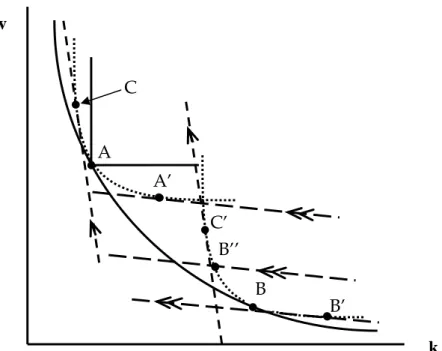
In Figure 1 below, we have depicted a putty-semi-putty production structure. The solid convex curve through points A and B is the unit iso-quant describing how much of the fixed factor (denoted by k) and of the variable factor (denoted by v) should be combined to produce one unit of output. This curve is the convex hull of numerous technologies that each have relatively limited substitution possibilities. Two of these technologies have been depicted using dotted curved lines in the Figure. They have the points A and B in common with their convex hull. They will further be called technologies A and B. A putty-clay model is a special case of this set-up, since in that case substitution possibilities ex post are zero by assumption. This is indicated, for example, by the solid rectangular iso-quant touching the hull in point A.9 This means that technology A effectively consists of just one technique, and so substitution between techniques (or moving along an iso-quant) is not
8 This assumes that the Inada conditions still apply in this case.
9 In a CES setting, the ex post iso-quant can be made to approach the rectangular iso-quant by choosing a value of the elasticity of substitution that is close to zero.
possible due to either the nature of the technology itself or the incompleteness of human knowledge.
It should be noted that this convex hull is a kind of short-hand notation for all the technologies that an entrepreneur can choose from. But once a particular technology like A or B has been chosen, further selections of techniques belonging to technologies A and B are limited to the ones represented by the dotted unit quants through points A and A’ or through points B and B’. The dotted unit iso-quants can therefore be thought of as collections of (slightly) different implementations of a particular technology. It should finally be noted that due to embodied factor augmenting technical change, the convex hull shifts in the direction of the origin. If factor augmenting technical change would be k-biased, then it shifts more in the direction of the k-axis than in the direction of the v-axis, and the other way around, mutatis mutandis.
Figure 1. A putty-semi-putty production structure
Technology A is relatively v-intensive implying that for the same relative prices, as is the case in points A’ and B’, for example, the v/k-ratio in point A’ is higher than the v/k-ratio in point B’. Hence, an entrepreneur who would expect the relative price of k to be generally low would be better off choosing technology B, and an entrepreneur who would expect the relative price of v to be low, would do better choosing technology A. This follows directly from the interpretation of the slope of
C’
B’
B’’
A’
B
A
v
k
C
the straight lines through points A’, B’ and B’’ as the relative factor prices of the factors v and k. In that case, the intercepts of the straight lines with the vertical are a direct measure of the total cost of v and k taken together. In that case point A’ represents a higher cost level than point B’, even though relative prices are the same in points A’ and point B’ (i.e. at relatively low relative prices for factor k). So why would technology A then ever be chosen? The answer is that entrepreneurs may expect factor prices to change ex post. And A would be the preferred technology if the factor price of v would be expected to be relatively low, even though it may be at a relatively high level at the moment the vintage is installed, as given by the slopes of the iso-cost lines through points B’ and A’, for example. So if the relative price of v is initially high but is also expected to be permanently much lower in the near future, them technology A is preferred to B by rational entrepreneurs.
If we would be using CES functions to describe both the ex ante unit-isoquant through points A and B (that is the convex hull of all individual technologies that are best practice at some point in time), and the unit iso-quants of all individual technologies like A and B, then the position of the individual technologies A and B in the factor coefficient space depends on the way in which the convex hull has been parameterised. In the context of a CES function, the general shape of the unit-isoquant depends the elasticity of substitution and the distribution coefficients. The values of these parameters implicitly define the position of the individual technologies A and B (and all other technologies supported by the hull). In addition to this, the shape of the individual technologies is of course defined by the elasticity of substitution associated with each individual technology. Take technology A, for example. Its distribution coefficients are completely determined by the requirements that the ex ante function and the ex post function must have a value equal to 1 in point A. Moreover, the slopes of the straight lines that are tangent in A with both the ex ante and the ex post unit iso-quants should be the same. These requirements are sufficient to define the ex post distribution coefficients of A in terms of the distribution coefficients of the ex ante function and the value of the ratio in point A. We will call this value of the v/k-ratio the ‘tangential technique’. Obviously, for technology B, the distribution coefficients would be defined in terms of the ex ante distribution coefficients and the v/k-ratio in point B.
The problem of choosing a technology to invest in then boils down to making two ‘sub-choices’: first the choice of an individual technology (like the unit ex post
iso-quant going through point B), and secondly a specific implementation of that technology (or individual techniques like B’ or B’’). In order to show how this works, we will have to specify the ex ante and ex post functions, after which we can specify the general investment problem and its solution. This is the subject of the following sub-paragraphs.
3.2 Defining the investment program
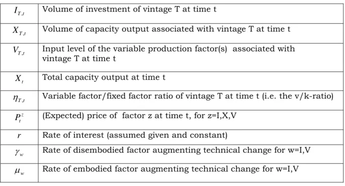
Before specifying the full investment decision process, we have to define the concepts and variables we are going to use. This is done in Table 1. below.
t T
I
, Volume of investment of vintage T at time tt T
X
, Volume of capacity output associated with vintage T at time tt T
V
, Input level of the variable production factor(s) associated withvintage T at time t
t
X
Total capacity output at time tt T,
η
Variable factor/fixed factor ratio of vintage T at time t (i.e. the v/k-ratio)z t
P
(Expected) price of factor z at time t, for z=I,X,Vr
Rate of interest (assumed given and constant)w
γ
Rate of disembodied factor augmenting technical change for w=I,Vw
μ
Rate of embodied factor augmenting technical change for w=I,VTable 1. Variables and parameters
There are two production functions that are relevant for each individual vintage of investment: the ex post function and the ex ante function (i.e. the convex hull of all ex post functions). Both are assumed to be linear homogeneous CES functions. The ex ante function has a higher elasticity of substitution between factors than the ex post function (otherwise it couldn’t be the convex hull of the ex post functions, since it would be more curved than the ex post functions that it should ‘envelop’). Both the unit iso-quants of the ex ante and the ex post functions of vintage v ‘touch’ (initially) at a certain value of v/k. Due to disembodied technical change taking place after the installation of a vintage, the ex post unit iso-quant may drift away from its initial position. Because ex post only the techniques from the ex post unit iso-quant are available to entrepreneurs wanting to use a particular technology, they have to make sure to choose the ‘right’ ex post iso-quant (or ‘tangential technique’), since that determines their ex post potential to absorb (expected) changes in factor prices that has a negative impact on overall profitability that is as small as possible.
As regards this profitability, we assume now that entrepreneurs want to maximise the present value of the rents they can obtain by investing in a certain technology and then using that technology as an integral part of their ‘vintage-portfolio’ to produce an aggregate volume of output needed to service demand. The decision how much to invest and in which ex post unit iso-quant to invest is made conditional on the requirement that the specific vintage investment is part of a complete intertemporal investment program10 with the aim of maximising the present value of the flow of rents that can be obtained from the vintage portfolio. In order to derive this investment program, we postulate the following ex ante and ex post production functions:
{
} {
}
(
α α)
1/α , , , , , ( , ) − − − ⋅ + ⋅ = = T TT TT T TT T TT T T g I V A I B V X (1.A){
} {
}
(
C
I
D
V
)
t
T
V
I
f
X
Tt=
Tt Tt Tt=
Tt⋅
Tt+
Tt⋅
Tt∀
≥
− − −β β 1/β , , , , , , , ,(
,
)
(1.B)In (1.A),
σ
a=
1
/(
1
+
α
)
is the elasticity of substitution of the ex ante function gT(),while
σ
p=
1
/(
1
+
β
)
is the elasticity of substitution of the ex post function fT,t() (cf.(1.B)). In equation (1.A), AT and BT are the ex ante distribution parameters that may
change over time (and so differ between technologies) due to embodied technical change, i.e.: T T I
e
A
A
=
0⋅
μ ⋅ (1.C) T T Ve
B
B
=
0⋅
μ ⋅ (1.D)Due to technical wear and tear, the amount of capital associated with a particular vintage gradually decays over time. We assume radioactive decay at a common rate
δ
for all vintages. Thus we get:T t e I IT,t = T,T ⋅ −δ⋅(t−T) ∀ ≥ (2)
10 An investment program is a sequence of investment decisions that optimises some objective
Because of the linear homogeneity of (1.A) and (1.B) we must have:
)
,
(
1
=
g
Tk
T,Tv
T,T (3.A))
,
(
1
=
f
T,tk
T,tv
T,t (3.B)where kT,t and vT,t are capital per unit of capacity output and the variable factor per
unit of capacity output of vintage T at time t. Initially, the two unit iso-quants should be tangent at the tangential technique given by
η
T,T =kT,T/vT,T. In addition,the slopes of both unit iso-quants should be the same for the tangential technique
T T,
η
. Hence we obtain the following constraints on gT () and fT,t():1 ) , ( ) , ( T,T T,T = T,T T,T T,T = T k v f k v g (4.A) T T T T T T T T T T T T T T
v
f
k
f
v
g
k
g
, , , , , ,/
/
∂
∂
∂
∂
=
∂
∂
∂
∂
(4.B)where (4.B) can be derived from the equal slopes requirement. (4.A) and (4.B) provide two equations that can be used to link the ex post distribution parameters to the ex ante distribution parameters for a given tangential technique
T T T T T T, =k , /v ,
η
and for given values of the substitution parameters α andβ
. We get:( )
α β β β α ( )/ , / , −⋅
=
T TT T TA
k
C
(5.A)( )
α β β β α ( )/ , / , −⋅
=
T TT T TB
v
D
(5.B)(5.A) and (5.B) describe the initial values of the ex post distribution parameters. These can change due to disembodied technical progress. It should be noted that the ex post parameters are equal to their ex ante counterparts if the elasticities of substitution ex ante and ex post are the same, as it should be in that case. Because of disembodied factor augmenting technical change at given rates
γ
I andγ
V , we have furthermore:) ( , , T t T T t T I e C C = ⋅ γ ⋅ − (6.A) ) ( , , T t T T t T V e D D = ⋅ γ ⋅ − (6.B)
The instantaneous flow of quasi-rents associated with investment in a certain vintage T at time t is now given by:
t T V t t T X t t T P X P V QR , = ⋅ , − ⋅ , (7)
It should be noted that from a vintage point of view there are two types of instrumental variables: those that can be determined only once (like the initial level of investment associated with a vintage, as well as the corresponding tangential techniques of that vintage), and those that can be adjusted ex post, like the ex post factor coefficient (and hence output too for an ex post given volume of investment). A third type of variable is non vintage-specific. In this particular case that would be the price of output (this assumes that output produced on all vintages is homogeneous). In equation (7), the ‘adjustable’ instrumental variables for time t are the price of output X
t
P
, capacity output of the existing vintages XT,t and the amountof the variable factor per vintage, VT,t. For the time of installation of the vintage T,
the ‘one shot’ instrumental variables are the volume of investment at time T, i.e.
T T
I
, , but also the tangential techniqueη
T,T =kT,T /vT,T that defines both the shapeand the location in factor-space of the ex post production function fT,t().
The demand for output Dt is assumed to be given by a constant
price-elasticity of demand function:
( )
−ε⋅
=
X t t tZ
p
D
(8)where Zt is an autonomous scale factor that may change over time, and where
ε
isa constant number greater than 1.
For reasons of simplicity and expositional purposes we now assume that investment decisions are taken continuously, rather than at one-year intervals. Furthermore, taking time t to refer to the present, we now want to find the investment program that maximises the present value of all current and future rent streams associated with all presently existing vintages and all the vintages still to be installed. Equation (9) contains the present value of the rents of all past, current
and future vintages installed and to be installed. In equation (9),
λ
t,
ξ
v,t,
ψ
v,t,
ϕ
t arethe Lagrange multipliers associated with the demand constraint, the ex post production function constraint, the requirement of the ex post fixedness of the volume of capital per vintage (apart from technical wear and tear) and the ex ante production function constraint, respectively.
Φ
t is the present value of the stream of rents from time t associated with all past, present and future vintages (to be) installed. For the vintages already installed at time t (i.e. all vintages with indext
T < ), only the factor proportions ex post can be changed. For the new vintages
(with vintage index T ≥t) the level of investment as well as the tangential technique
and the ‘actual’ techniques can be chosen at the moment of installation of these new vintages.
(
)
(
)
∫
(
)
∫
∫
∫
∫
∫
∫
∫
∫
∞ = −∞ = − ⋅ − ∞ = −∞ = ∞ = ∞ = =−∞ −∞ = ∞ = − ⋅ −−
⋅
+
−
⋅
⋅
+
−
⋅
+
⎟⎟
⎠
⎞
⎜⎜
⎝
⎛
−
⋅
+
⎟⎟
⎠
⎞
⎜⎜
⎝
⎛
⋅
−
⋅
−
⋅
⋅
=
Φ
t t t t t t t t t T t T T t T T t T t t t T t T t T t T t T t T t t t t t T t T x t t t t T t t I t t T V t t T X t t t t t r tdt
v
k
g
dt
dT
I
e
I
dt
dT
X
V
I
f
dt
dT
X
p
D
dt
I
p
dT
V
P
X
P
e
1 1 , 1 1 , 1 1 1 1 1 , ) 1 ( , 1 , 1 1 1 , 1 , 1 , 1 , 1 , 1 1 1 1 , 1 1 1 1 1 , 1 1 1 , 1 1 , 1 1 ) 1 (1
)
,
(
1
1
1
)
,
(
)
(
1
)
(
ϕ
ψ
ξ
λ
δ (9)Hence, we find as first order conditions for an old vintage T at some moment in time
t t1≥ that: 1 , 1 , 1 ) 1 ( 1 , 1 , 1 , 1 , 1 ) 1 ( 1 , 1 , 1 ) 1 ( 1 , 1 , 1
0
t T t T V t t t r t T t T t T t T V t t t r t T t T V t t t r t T t T tX
V
P
e
V
V
f
V
P
e
V
f
P
e
V
Δ
Δ
⋅
⋅
≈
Δ
⋅
∂
∂
Δ
⋅
⋅
=
∂
∂
⋅
=
=>
=
∂
Φ
∂
−⋅ − −⋅ − −⋅ −ξ
(10.A) 1 , 1 , 1 , 1 , 1 , 10
t T t T t T t T t T tI
f
I
∂
∂
⋅
=
=>
=
∂
Φ
∂
ψ
ξ
(10.B) 1 1 ) 1 ( 1 , 1 , 0 Tt rt t tX t t T t P e X = =>ξ
= ⋅ −λ
∂ Φ ∂ − −⋅ (10.C)Equation (10.A) shows that the Lagrange multiplier
ξ
T,t1 can be interpreted as the marginal variable cost of the marginal unit of output on vintage T at time t1. Note that (10.C) should hold for all T ≤t1. Moreover, the RHS of (10.C) isindependent of T, and so it must be the case that
ξ
T,t1=
ξ
t1,t1∀
T
≤
t
1
. Hence on oldand new vintages the variable factors should be employed up to the point where their marginal product is the same on all vintages.
For a new vintage at the time of its installation t1 we find for the initial volume of investment that:
2 0 1 2 2 . 1 ) 1 2 ( 1 ) 1 .( 1 , 1 dt e p e I t t t t t t I t t t r t t t
∫
∞ = − ⋅ − − − ⋅ = ⋅ => = ∂ Φ ∂ δψ
(11)It should be noted that (11) can be written in a somewhat more familiar format by differentiating (11) with respect to time t1, using Leibniz’s rule for differentiating integrals. To do this, we use the definition I
t I I
t
dt
p
p
dp
1/
1
=
ˆ
⋅
1 where ahat over a variable denotes the proportional rate of growth of that variable. Thus we get: ) ˆ ( 2 1 1 ) 1 .( 1 , 1 1 2 2 . 1 ) 1 2 ( 1 , 1 1 ) 1 .( I I t t t r t t t t t t t t t t I t t t r P r P e dt e dt P e d − + ⋅ ⋅ = ⇔ ⋅ ⋅ + − = ⋅ ∞ − − = − ⋅ − − −
∫
ψ
ψ
δ
δ
ψ
δ (12)Equation (12) implies that
ψ
t1,t1 is the expected user cost of capital as it is usually defined, except for the fact that it is discounted from time t1 until time t (the moment at which the investment program is formulated).Using (10.A) and (10.B) together with Euler’s equation, we find for a new vintage at the moment of its installation t that:
(
)
(
1 1,1 1 1,1)
) 1 .( 1 , 1 1 , 1 1 ) 1 .( 1 , 1 1 , 1 1 , 1 1 , 1 1 , 1 1 , 1 1 , 1 1 , 1 1 , 1 1 , 1 1 , 1ˆ
t t V t t t I t I t t r t t t t V t t t r t t t t t t t t t t t t t t t t t t t t t tv
P
k
P
P
r
e
V
P
e
I
X
I
I
f
V
V
f
⋅
+
⋅
⋅
−
+
⋅
=
⇒
⋅
⋅
+
⋅
=
⋅
=
⎟
⎟
⎠
⎞
⎜
⎜
⎝
⎛
⋅
∂
∂
+
⋅
∂
∂
⋅
− − − −δ
ξ
ψ
ξ
ξ
(13)Note that
ξ
t1,t1 is actually the present value of unit total cost of the newest vintage installed at time t1. Hence, combining (13.A) with (10.A), while recalling that1
1 , 1 1 ,t t tT
t
T=
ξ
∀
≤
ξ
, we have:(
)
(
)
1 ,1 ,1 ,1 ) 1 .( 1 , 1 1 1 , 1 1 ) 1 .( 1 , 1ˆ
/(
Tt/
Tt)
Tt V t t t r t t V t t t I t I t t r t te
r
δ
P
P
k
P
v
e
P
f
V
ξ
ξ
=
− −⋅
+
−
⋅
⋅
+
⋅
=
− −⋅
∂
∂
=
(14)Equation (14) says that factor proportions on old and new vintages should be adjusted in such a way that the marginal variable cost on old vintages (cf. equation (10.A)) should be exactly equal to the unit total cost on new vintages (due to the linear homogeneity of the production function ex post, this is also the marginal total cost on the new vintage). This is also what the Malcomson scrapping conditions says in case of a putty-clay or clay-clay vintage model (Malcomson 1975). Equation (14) is therefore a generalisation of the original Malcomson scrapping condition. The logic of this condition is that if total unit costs on a new vintage are lower than marginal variable cost on an old vintage, then the difference between these costs can be saved (and hence profits can be increased by the same amount, ceteris paribus) by transferring the marginal unit of output from the old vintage to the new one. By means of this transfer, marginal variable costs on the old vintage will fall (due to the rise in the marginal product of the variable factor), and the marginal total cost on the new vintage stays the same by assumption (due to the linear homogeneity of the relevant new production technology). This transfer should stop when the marginal variable costs on all old vintages would be equal to the marginal total unit cost on the new vintage. In the latter case no further cost savings can be made by transferring output from the old to the new vintage.
In order to show how this ‘scrapping’ condition as given by (14) is related to the negative quasi-rent condition11, it is instructive to find the optimum time-path for the price of the output produced using the investment program first. We have:
1 1 ) 1 .( 1 1 1 1 1 , ) 1 .( 1
0
0
t X t t t r X t t t t T t T t t r X t tP
e
P
D
dT
X
e
P
λ
∂
=
⇒
⋅
=
ε
⋅
λ
∂
⋅
−
⋅
=>
=
∂
Φ
∂
− − −∞ = − −∫
(15)11 This is an alternative scrapping condition that says to stop using a vintage when its quasi-rents start to become negative.
where we have used equation (8). Substituting (15) into (10.C) and taking account of (14), we find:
(
)
(
1 1,1 1 1,1)
1ˆ
1
t t V t t t I t I X tr
P
P
k
P
v
P
⋅
+
−
⋅
⋅
+
⋅
−
=
δ
ε
ε
(16)Equation (16) reproduces the Amoroso-Robinson condition for the profit maximising price of output under imperfect competition. If the price elasticity of demand is infinitely high (as it would be the case in a perfectly competitive environment), then the optimum price just covers marginal total cost, and hence equation (14) would in this case be reduced to the non-negative quasi-rent condition. This follows readily from the fact that in that case the price of output would equal total unit cost on the newest vintage, and so equation (14) states that the variable factor should be adjusted up to the point where the marginal variable costs just equal the price of output (and hence (marginal) quasi-rents on the old vintages are zero). Note that in the case of a putty-clay model, this rule implies that the allocation of the variable factor to machinery of an old vintage should be reduced as long as its marginal variable cost exceeds the price of output. Since in a standard putty-clay model the factor productivities ex post are independent of the level of use of the factors under consideration, this means that the input of the variable factor should be reduced to a zero level, hence effectively ‘scrapping’ the entire vintage.
We conclude then that equation (14) generates qualitatively the same results as the scrapping rules one normally encounters in clay-ex-post vintage models. Equation (14) is conceptually similar, but is more general since it covers putty-semi-putty models as well. Moreover, equation (14) has the benefit of resulting from a general intertemporal optimisation problem rather than being postulated a priori.
3.3 Choosing the optimum ex post iso-quant in a putty-semi-putty situation
Because of the fact that the volume of investment, once chosen, remains fixed (apart from technical decay), whereas the variable factor intensity can change ex post, it follows that investment decisions need to be made conditional on what is expected to happen in the future. This can be done as follows.
First differentiate (9) with respect to the determinants of the tangential techniques
k
T,T andv
T,T. We get:0 2 0 1 , 1 1 1 1 2 1,1 2 , 1 2 , 1 1 , 1 = ∂ ∂ ⋅ − ∂ ∂ ⋅ => = ∂ Φ ∂
∫
∞ = t t t t t t t t t t t t t t t k g dt k f kξ
ϕ
(17.A) 0 2 0 1 , 1 1 1 1 2 1, 2 , 1 2 , 1 1 , 1 = ∂ ∂ ⋅ − ∂ ∂ ⋅ => = ∂ Φ ∂∫
∞ = t t t t t t t t t t t t t t t v g dt v f vξ
ϕ
(17.B)Because of the linear homogeneity of the ex ante function
g
t(
)
, we also find that:2
1 2 1 , 1 1 , 1 2 , 1 1 , 1 1 , 1 2 , 1 2 , 1 1k
dt
k
f
v
v
f
t t t t t t t t t t t t t t t t t∫
∞ =⎟
⎟
⎠
⎞
⎜
⎜
⎝
⎛
∂
∂
+
∂
∂
⋅
=
ξ
ϕ
(18)Using equations (1.B), (1.C), (1.D), (5.A),(5.B),(6.A), (6.B) and the requirement that
ξ
T,t1=
ξ
t1,t1∀
T
≤
t
1
, and taking account of (13), it follows that (18) can be writtenas: 2 1 2 2 , 1 2 , 1 1 X dt t t t t t t t
∫
∞ = ⋅ ⋅ − =ξ
β
β
α
ϕ
(19)It follows from (19) that
ϕ
t1 is proportional to the present value of the cost associated with producing output on the vintage installed at time t during its entire (infinite) lifetime. It should be noted that the bigger the difference is between the elasticities of substitution ex ante and ex post, the largerϕ
t1 will be. In theputty-putty case we have
α
=
β
⇒
ϕ
t1=
0
∀
t
1
. In this case substitution possibilities expost are as large as those ex ante, and so an optimum tangential technique does not exist. Equation (19) by itself is of little real help in determining the optimum tangential technique, though. But equations (10.A) and (10.B) in combination with (17.A) and (17.B) provide the information we need. Taking the ratio of equations (17.A) and (17.B), we find:
α α
ψ
ξ
ξ
/ 1 1 2 2 , 1 2 ) 1 2 .( 1 2 2 , 1 2 , 1 1 1 1 , 1 1 , 1 1 , 1 1 2 2 , 1 2 , 1 1 , 1 1 2 2 , 1 2 , 1 1 1 , 1 1 , 1 1 1 1 , 1 1 1 , 1 12
2
2
/
2
/
/
/
− ∞ = − − ∞ = ∞ = ∞ = − −⎪
⎪
⎭
⎪
⎪
⎬
⎫
⎪
⎪
⎩
⎪
⎪
⎨
⎧
⋅
⋅
⋅
=
⎟
⎟
⎠
⎞
⎜
⎜
⎝
⎛
⇒
∂
∂
⋅
∂
∂
⋅
=
⎟
⎟
⎠
⎞
⎜
⎜
⎝
⎛
⋅
=
∂
∂
∂
∂
∫
∫
∫
∫
dt
V
p
e
dt
I
A
B
v
k
dt
v
f
dt
k
f
v
k
B
A
v
g
k
g
t t t t V t t t r t t t t t t t t t t t t t t t t t t t t t t t t t t t t t t t t t t t t t t t t (20)Equation (20) can be obtained by substituting (10.A) and (10.B) into (17.A) and (17.B), while noting that the marginal products of the tangential techniques can be related directly to the ex post marginal productivities of capital and the variable factor(s). Equation (20) shows that the capital intensity of the optimum tangential technique depends negatively on the ratio of the present value of the total capital costs associated with a vintage (i.e. the numerator of the last part of equation (20)) and the present value of total variable costs necessary to use the vintage (i.e. the denominator of the last part of equation (20)).
In order to fully solve equation (20) for the tangential technique, we need to solve two other ‘problems’ first. We need to find the value of
ψ
t1,t2 and also the value ofV
t1,t2/
I
t1,t2. This follows immediately from the fact that we can write the second part of (20) as: α δ δψ
/ 1 1 2 2 , 1 2 , 1 ) 1 2 ).( ˆ ( 1 ) 1 2 .( 1 2 ) 2 ( 2 , 1 1 1 1 , 1 1 , 1 2 ) / ( 2 − ∞ = − − + − − − ∞ = − ⋅ − ⎪ ⎪ ⎭ ⎪ ⎪ ⎬ ⎫ ⎪ ⎪ ⎩ ⎪ ⎪ ⎨ ⎧ ⋅ ⋅ ⋅ = ⎟ ⎟ ⎠ ⎞ ⎜ ⎜ ⎝ ⎛∫
∫
dt I V e P e dt e A B v k t t t t t t t t P r V t t t r t t t t t t t t t t t t V (21)It should be noted that the integral in the numerator of the RHS of (21) is exactly equal to the present value price of capital (see equation (11)), whereas
2 , 1 2 , 1t
/
t t tI
2 , 1 2 ) 1 2 .( 1 2 , 1 2 , 1 2 , 1 2 , 1 2 , 1 2 , 1 2 , 1 2 , 1
/
/
t t V t t t r t t t t t t t t t t t t t t t te
P
I
V
C
D
I
f
V
f
ψ
β⋅
=
⎟
⎟
⎠
⎞
⎜
⎜
⎝
⎛
⋅
=
∂
∂
∂
∂
− − − − (22)where it should be noted that the ex post distribution parameters Ct1,t2 and Dt1,t2
depend on the tangential technique again. It follows from (22) that we need to know what
ψ
t1,t2 looks like.Let us assume now that ˆ(2 1) 1 , 1 2 , 1 t t t t t t e − ⋅ ⋅ =
ψ
ψψ
. Substituting this into equation (11), we find that: 1 , 1 ) 1 .( 1 , 1 1 2 ) 1 2 ( ). ˆ ( 1 , 1 1 2 ) 1 2 ( 2 , 1 2 2 /( ˆ) ( ˆ) t t I t t t r t t t t t t t t t t t t t t e dtψ
e dtψ
δ
ψ
e Pδ
ψ
ψ
ψ
⋅ δ = ⋅ ∞ δ ψ = − ⇒ − − ⋅ ⋅ − = = − ⋅ − − ∞ = − ⋅ −∫
∫
(23)Obviously, (23) and (12) taken together imply that
ψ
ˆ=PˆI −r. Substituting the latterresult into (22), we get:
2 , 1 ) 1 /( ) ( 1 , 1 1 , 1 ) 1 /( 1 1 2 , 1 ) 1 2 ).( ˆ ˆ ( 1 2 , 1 2 , 1 2 , 1
)
ˆ
(
t t t t t t I I t t t t t P P V t t t t t t tk
v
P
r
P
D
e
P
C
I
V
V IΩ
⋅
⎟
⎟
⎠
⎞
⎜
⎜
⎝
⎛
=
⎟
⎟
⎠
⎞
⎜
⎜
⎝
⎛
−
+
⋅
⋅
⋅
⋅
=
⎟
⎟
⎠
⎞
⎜
⎜
⎝
⎛
− − − +β α−β +βδ
(24)where we have defined:
) 1 /( 1 1 1 ) 1 2 )).( .( ˆ ˆ ( 1 1 2 , 1
)
ˆ
(
β γ γ βδ
+ − − − − −⎟
⎟
⎠
⎞
⎜
⎜
⎝
⎛
−
+
⋅
⋅
⋅
⋅
=
Ω
I I t t t t P P V t t t tP
r
P
A
e
P
B
V I V I (25)Substituting (24) and (25) into (21), and solving for the tangential technique, we finally obtain: 1 ) 1 /( 1 / 1 / ) 1 ( 1 1 1 1 1 , 1 1 , 1 ) ˆ ( 1 ˆ ) ˆ ( ) ( ) 1 ( t I I V I V V t I t t t t t t t W P r P P r P P A B v k = ⎪⎭ ⎪ ⎬ ⎫ ⎪⎩ ⎪ ⎨ ⎧ − + ⋅ ⎟⎟ ⎠ ⎞ ⎜⎜ ⎝ ⎛ + − − − ⋅ + + ⋅ + ⋅ ⋅ ⎟⎟ ⎠ ⎞ ⎜⎜ ⎝ ⎛ = ⎟ ⎟ ⎠ ⎞ ⎜ ⎜ ⎝ ⎛ −α +β β − β − +α
δ
β
γ
γ
β
δ
β
(26)Equation (26) shows how the elasticity of substitution and the distribution parameters of the ex ante function, together with the structural parameters of the ex post function determine the optimum choice of the tangential technique. We see that high rates of disembodied capital augmenting technical change will tend to increase the capital intensity of the tangential technique. Something similar goes for the other factor(s) of production too. Equation (26) also shows what happens if the elasticity ex post goes to zero (i.e. if
β
→
∞
). In that case we find that:) 1 /( 1 1 1 1 1 1 , 1 1 , 1 ) ˆ /( α α
γ
γ
δ
+ − − ⎪⎭ ⎪ ⎬ ⎫ ⎪⎩ ⎪ ⎨ ⎧ − − + + ⋅ ⎟⎟ ⎠ ⎞ ⎜⎜ ⎝ ⎛ = ⎟ ⎟ ⎠ ⎞ ⎜ ⎜ ⎝ ⎛ V I V V t I t t t t t t t P r P P A B v k (27)and we see that the tangential technique would be determined by the ratio of the present value of the costs associated with buying (i.e. the numerator of the rightmost term within the curly brackets of (27)) and operating (i.e. the denominator of the aforementioned term) the tangential technique.12 Because of the ex post clay assumption made here, the tangential technique is actually the point where a rectangular isoquant touches the hull, as for example in point A in Figure 1.
Given the value of Wt1 (cf. equation (26)), we can now determine the individual components of the tangential technique directly from equations (26) and (3.A), giving:
(
α)
1/α 1 1 1 1 , 1t t t t t A W B v = ⋅ − + (28.A)(
α)
1/α 1 1 1 1 1 , 1t t t t t t W A W B k = ⋅ ⋅ − + (28.B)Equations (28.A) and (28.B) finally allow us to identify the ex post production functions/technologies that will be chosen at any point in time. Hence we can now also determine the allocation of the variable factor to the fixed factor capital on all
12 The price of investment goods is equal to the present value of the user cost of capital discounted at the ruling interest rate, since
∫
⋅( + )⋅ =1∞ ⋅ − ⋅ −rt t e r e
δ
δ .existing and new vintages, given our knowledge about the exact position in factor-space of the ex post functions. Consequently, we are also able to calculate how much output would still be produced on all existing vintages after ‘scrapping’ non profitable capacity on those vintages thus obtaining the capacity gap to be filled by the new vintage. This follows readily from the application of Leibniz’s rule to required aggregate capacity output Xt. Differentiating capacity output with respect to time t, we get:
∫
∫
∫
= = = ∂ ∂ − = ⇒ ∂ ∂ + = = t T t T t t T t t t T t T t t t T t dT t X dt dX X dT t X X dT X dt d dt dX 0 , 0 , , 0 , , (29)In equation (29), T is the vintage index, and t is the current time for which we have to determine the required volume of investment. It is furthermore assumed here that capital has been accumulated from time zero. Equation (29) states that the capacity of the newest vintage at time t should be large enough to service the gross increase in the demand for capacity output (dX/dt), less the extra capacity output that can be obtained from existing capacity due to technical change, amongst other things. Indeed, if the extra output on old vintages is negative, because of technical wear and tear or an increase in the capital intensity of production due to technology induced ‘scrapping‘, for instance, then the required amount of new capacity output increases one for one, and so does the volume of new investment, ceteris paribus. So the investment equation associated with (29) is:
t t t t t t
X
k
I
,=
,⋅
, (30)The logic of the model can now be summarised as follows. Expectations regarding factor price developments and (biases in) technical change determine the tangential technique at any moment in time. Current price ratios then determine factor ratios given the choices of the ex post functions implied by the various tangential techniques. These factor ratios together with the amount of capital tied up in old vintages determine the level of capacity output on each old vintage. Consequently, aggregate capacity output can be obtained by aggregation over all old vintages. The average total unit cost together with the Amoroso-Robinson mark-up-rule determines output prices, hence demand. The difference between total demand
and the part of demand that is met using old vintages then needs to be filled by new capacity.
4. The putty-practically-clay model
4.1 Introduction
The model outlined in the previous section, has the putty-clay model as a special case for
β
→
∞
, as shown by equation (27), for example. In that case the elasticity of substitution between the fixed and the variable factors becomes zero, and the ex post iso-quant becomes rectangular. Only due to disembodied technical change ex post, factor ratios may change. As stated earlier, a full putty-clay model requires the explicit scrapping of marginal units of investment on old vintages whenever and as long as their marginal variable cost exceed the marginal total production cost of that same unit of output on the newest vintage. The problem in this case is that both old and new vintages are homogeneous by assumption. For a given scrapping rule in a clay ex post context, this implies that an entire vintage is operated or not. This leads to discontinuities in the aggregate supply function. The latter can lead to numerical difficulties when solving a CGE model containing such a vintage model as its production block.There is a fix to this problem that entails the assumption of heterogeneity within vintages. The latter implies, again for a given scrapping rule, that the least productive machinery belonging to a vintage may be scrapped before the more productive machinery. This increases the smoothness of the response of the aggregate supply function to price changes. The problem with this fix is that it creates infinitely many vintages, and it is hard to keep track of which sub-vintages are operated and which aren’t in an efficient way.
An alternative fix is to assume a large value of