http://www.sciencepublishinggroup.com/j/earth doi: 10.11648/j.earth.20190805.14
ISSN: 2328-5974 (Print); ISSN: 2328-5982 (Online)
1D Inversion of Large Loop Transient Electromagnetic Data
Acquired Using Offset Loop Configuration Over Multi-layer
Earth Models
Satya Prakash Maurya, Nagendra Pratap Singh
*, Ashish Kumar Tiwari
Department of Geophysics, Institute of Science, Banaras Hindu University, Varanasi, (U. P), India
Email address:
*Corresponding author
To cite this article:
Satya Prakash Maurya, Nagendra Pratap Singh, Ashish Kumar Tiwari. 1D Inversion of Large Loop Transient Electromagnetic Data Acquired Using Offset Loop Configuration Over Multi-layer Earth Models. Earth Sciences. Vol. 8, No. 5, 2019, pp. 285-293.
doi: 10.11648/j.earth.20190805.14
Received: September 14, 2019; Accepted: October 15, 2019; Published: October 25, 2019
Abstract:
The present research describes a 1D inversion scheme for interpretation of large loop TEM data acquired using offset loop configuration due to a large loop source, over the layered earth models. The inversion is based on a non-linear least square method that generates a smooth layered earth model by minimizing the residual misfit function in an iterative process. It produces an inverted model from the data using the criteria of minimization of misfit function and/or convergence of residual in two successive iterations. The forward problem is formulated in frequency domain, and then it is transformed into the time domain using Fourier cosine and sine transform. The accuracy and robustness of algorithm is tested by inverting the large loop TEM data acquired using offset loop configurations over the homogeneous, two layer, three layer and four layer earth models, with or without the addition of random noises. Inverted results are in good accordance with the theoretical models and validate that different parameters are recovered with high accuracy. The program works satisfactorily with noisy data and produces inverted results with acceptable accuracy for synthetic data up to 5% random noises.Keywords:
Large Loop TEM Methods, Layer Earth Model, Offset Loop Configuration, Inverse Modeling1. Introduction
Conductivity-depth inversion has proven to be a useful tool in mapping the distribution of geologic conductivity and identification of conductive sources within the variably conductive host geology. There are number of methods for deriving conductivity-depth sections from time-domain EM data [1-4] based on different approaches. Of the various conductivity depth techniques, each one is meant for the specific case and is suitable for a particular source excitation (i.e. impulse/step/saw tooth wave etc.), survey configuration (central loop or coincident loop configuration) and is not amenable to its adoptability for commercially used other TEM systems except for the particular one for which it is developed.
Moreover, among the various transient electromagnetic (TEM) methods, the large loop TEM methods represents a
offset loop configurations. Therefore, in the present study an attempt is made to develop an inversion technique for interpretation of large loop transient data acquired using offset loop configuration.
There are various techniques available in literature for inverse modeling of TEM data (voltage decay curve) [1, 3, 4, 23-36, 39]. Off all these techniques, none is suitable for inverting the large loop TEM data acquired using offset loop configurations. In present work, an attempt is made to develop a robust conductivity-depth inversion technique capable of generating conductivity variation with depth for TEM data acquired using large loop source (impulse excitation) for offset loop configuration due to a large loop source. In present work the continuous voltage versus time curve is inverted to generate conductivity variation with depth using the inversion concept similar to Anderson [43]. The conductivity-depth inversion and associated forward algorithms are developed for the interpretation of TEM sounding data acquired using offset loop configuration with provision of its adaptability to most widely used commercial TEM systems with different source excitation and survey configuration.
2. Theoretical Backgrounds
2.1. Forward Modeling
To achieve the objective, an inversion algorithm is developed to invert large loop TEM data acquired using offset loop configurations due to a large loop source over the layer earth models, and is tested for noise free and noisy data (with addition of random noise up to 5%) over homogeneous as well as layered earth models.
The large offset loop system presents a source loop and a smaller loop at an offset loop point depicts receiver position corresponding to the offset loop configuration.
In general, the data collected from a large loop TEM system consist of vertical voltage measurements at various time intervals after the current in transmitter is turned off. These voltage measurements are related to the time derivatives of vertical magnetic field in accordance with the following relation,
= − (1)
where M is the area-turns product of the receiver coil. These voltage data can be inverted directly for the layered earth models or it can be further transformed to the apparent resistivity and then inverted. Sometime it is preferable to use apparent resistivity transformation to have a direct relation with the geo-electrical section and for getting an initial estimate of layer resistivities which is often required for further non-linear inversion.
The forward solution for time derivative of vertical magnetic field is obtained by transforming the frequency domain solutions for the vertical magnetic field into the time domain solution using Fourier cosine or sine
transform ([14]),
= # , , ℎ cos ! (2)
= #$% , , ℎ sin ! (3)
Where , , ℎ and $% , , ℎ are the real and imaginary parts of the vertical magnetic field over a layered earth in frequency domain. The component of vectors and h are the resistivities and thickness of different layers of layered earth model, and is the angular frequency.
The frequency domain expressions of EM field components at a point on or above the surface of an n-layered earth due to a finite size horizontal circular loop of radius, a, carrying a current, I, and placed at the height, h, above the surface of layered earth is given in Ward and Hohmann [38]. The expression of ( field component at a measurement point on the surface of n-layered earth (i.e. at z = 0) can be written as,
, , ℎ =)* +,-./012345678
9/ :1 ;< : ;= !;
#
(4)
where =>?=@@/ @AB
/2@AB, with C =
9/
DEF/ (intrinsic admittance of free space)
and CG =1 H?I45 J45 = −
HJ45
?I45 (surface admittance at z = 0)
For an n-layer case, the surface admittance is given by the recurrence relation,
CA1= C1CA + CC 1tanh O1ℎ1 1+ CA tanh O1ℎ1
CAP= CPCACP21+ CPtanh OPℎP P+ CAP21tanh OPℎP
and CAP= CP, with CP=DEF9Q Q,
OP= RS+ RT− RP 1U = ; − RP 1U , and
RP= PVP− W PXP
Here, r is source-receiver offset (measured from center of the loop). For calculation purposes, tanh OPℎP is used in its exponential form for stability reasons [23].
Therefore, starting with computation of , , ℎ field (Eq. 4), using the algorithm described in [16], the time derivative of vertical magnetic field is computed using the Fourier cosine and sine transforms (Eqs. 2 and 3) [14, 26]. Thereafter, the voltage response is computed (Eq. 1) which is needed as forward computation in this inversion scheme.
2.2. Inversion Approach
problems, assumes an initial model, representative of the earth under the consideration. Thereafter, the model parameters are estimated using an optimization technique. The important aspect of the second approach is the assumption of correct class of model. This approach allows for geological and geophysical information to be incorporated into the inverse problems. However, the major disadvantage of this approach is that by assuming an initial model, there is always a chance of unknown bias introduced into the inverse problem [6].
The proposed inversion scheme is based on model fitting approach, where initial model is the layer earth with parameters consisting of resistivities and thicknesses of different layers. For inversion, it follows Anderson [37] approach with slight modification such as using EMLCLLER [16] in place of forward computation algorithm and changes in input parameters in accordance with need of the present problem and to overcome the practical limitations associated with the NLSTCI program [37] for the central loop case. This program is a modification of NLSTCI (nonlinear least-squares inversion of transient soundings for a central induction loop system) and of a general nonlinear least square algorithm of Dennis et al. [40] to that of a constrained and unconstrained algorithm with weighted observations, which is more reliable than a Gauss-Newton or Levenberg-Marquardt algorithm when a large residual exists between data and forward solution. To overcome the problem of local minima associated with NLSTCI, some adjustment have been made in the program that in next step it recalls the program by replacing initial model parameters with inverted parameters obtained in the previous step and repeat the process for the desired number of steps or till it get a reasonable model parameters. This is achieved through the use of the fact that at each step program start with new value of A (Marquardt parameter) depending upon the resulting residual at that step and some special procedures. The forward problem is based on Singh et al. [17] for homogeneous earth model and makes use of EMLCLLER [16] for FDEM calculation over layered earth model, which is entirely different to that in [37] program, which uses [22] algorithm for computation of central loop frequency domain response. The inversion is based on minimization of a residual misfit function in an iterative least square process. The misfit function, which is minimized in an iterative process, can be defined as following.
Y =1 Z[ (5)
Z[ =√P1 ∑ ^_= `ab $ c ∗ C $ − YP
De1 (6)
where Y (I) and WT (I) are the Ith data point and corresponding weight factor, and F is corresponding calculated value.
In this algorithm, we have used 1D model, because there is scarcity of reliable inversion scheme for layered earth which is always relevant because it gives general idea about the resistivity variation in the subsurface that can be used as
initial model for further advanced inversion schemes.
3. Results and Discussion
For checking the accuracy and efficiency of the program for inverting the large loop TEM sounding data, it is applied for the inversion of large loop TEM data acquired using offset loop configurations over the homogeneous, 2-layer, 3-layer and 4-3-layer earth models. The inversion is tested for the noise free as well as for noisy data (with addition of random noise), and relevant results are presented in Figures 1-4.
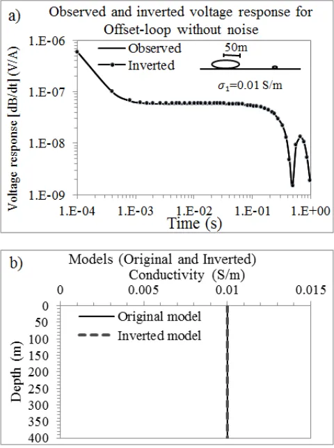
Figure 1 presents inversion results for the large loop TEM data for offset loop configuration over the homogeneous earth model. Figure 1(a) shows voltage response for a source loop of radius 50m and Figure 1(b) shows inversion results. The inversion was stared with an initial homogeneous model of conductivity 0.001 S/m for noise free, 1% random noise, 3% random noise and 5% random noise data, however, the results are presented only for noise free data. From Figure 1a, it is observed that there is good match between the original and inverted voltage response data; while Figure 1(b) depicts that the final inverted models are in good agreement with the original models with which data were generated. The conductivity of homogeneous layer is reproduced with a difference of as little as 0.1%.
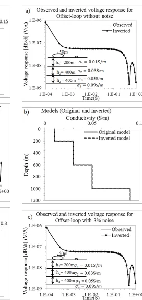
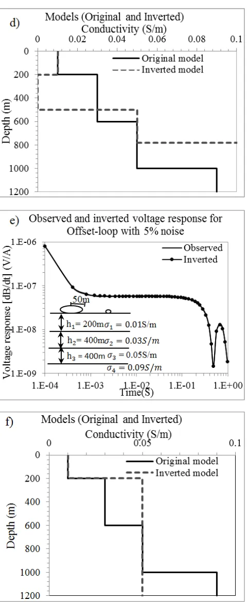
Figure 2 shows inversion results for the large loop TEM voltage response data over the 2-layer earth model for offset loop configuration. The source loop radius is 50m. Figures 2(a), 2(c) and 2(e) show the original and the inverted voltage response curves for noise free, 3% and 5% random noise data, respectively, and depicts that there is good matching between the original and inverted curves. Figures 2(b), 2(d) and 2(f) show original and inverted 2-layer conductivity models for noise free, 3% and 5% random noise in the data, respectively.
The inversion was started with a homogeneous earth model of conductivity 0.001S/m. The figures depict that there is good agreement between the inverted and original conductivity models with which data were generated. The inverted parameters, i.e. conductivities and thickness of different layers are close to the original parameters. The average variation of inverted parameters is less than 1%. These results depict accuracy and capability of the method for inversion of large loop TEM data acquired using offset loop configuration.
Thereafter, the algorithm is applied for inverting the voltage time data over a 3 layer earth model with addition of 1%, 3%, 5% and more than 5% random noises. However, the results up to 5% random noise are shown. Figure 3 depicts inversion results for the large loop TEM voltage response data over the 3-layer earth model for offset loop configuration. The source loop radius is 50 m. Figures 3(a), 3(c) and 3(e) show the original and the inverted voltage response curves for noise free, 3% and 5% random noise in the data respectively, and show that there is good match between the original and inverted curves. Figures 3(b), 3(d) and 3(f) show original and inverted conductivity models of 3-layer earth for noise free, 3% and 5% random noises in the data, respectively. The inversion was started with a homogeneous model of conductivity 0.001S/m. The figures depict that there is good agreement between the inverted and original conductivity model with which data was generated. The inverted parameters, i.e. conductivities and thickness of different layers are close to the original parameters. The average variation of inverted parameters is less than 4%. These results depict accuracy and capability of the method for inversion of large loop TEM data acquired using offset loop configuration. These results indicate the capability of the program to invert large offset loop TEM data over 3 layer earth models.
Figures 4 depict inversion results for the large loop TEM voltage response data over the 4-layer earth model for offset loop configuration for source loop of radius 50m. Figures 4(a), 4(c) and 4(e) show comparison of original and inverted voltage response curve for noise free, 3% and 5% random noise data, respectively. It is noticed that there is good match between the original and inverted curves. Figures 4(b), 4(d) and 4(f) show original and inverted 4-layer conductivity models for noise free, 3% and 5% random noise data respectively. The inversion was started with a homogeneous model of conductivity 0.001S/m. The figures depict that there is good agreement between the inverted and original models
Figure 2. Inversion results for offset loop TEM data over a 2-layer earth model where (a) depicts synthetic and inverted best fit data, (b) depicts original and inverted conductivity models for noise free TEM data. (c) The synthetic and inverted best fit data with 3% noise, (d) original and inverted conductivity models for 3% random noise, (e) depicts synthetic and inverted best fit data for 5% noise and (f) original and inverted conductivity models for TEM data with 5% random noise.
From results presented in Figures 1 to 4, it is noticed that the program is capable of interpreting large loop TEM data acquired using offset loop configurations over the homogeneous, 2-layer, 3-layer and 4-layer earth models and
Figure 4. Inversion results for offset-loop TEM data over a 4-layer earth model. (a) Compare synthetic and inverted best fit data, (b) original and inverted conductivity models for noise free TEM data, (c) compare synthetic and inverted best fit data for 3% noise, (d) original and inverted conductivity models for 3% random noisy data, (e) compare synthetic and inverted best fit data for 5% noise and (f) original and inverted conductivity models for TEM data with 5% random noise.
4. Conclusions
The present study embodies the results on inversion of large loop TEM data over layered earth model acquired using offset loop configurations with objective of presenting a suitable inversion scheme for interpretation of real field TEM sounding data acquired using large loop sources. An inversion scheme based on minimization of residual misfit function is developed and applied for the inversion of large loop transient electromagnetic (TEM) data. The developed inversion scheme is based on modification of NLSTCI program ([37]) in accordance with the need of the problem. Accordingly the forward computation scheme in NLSTCI has been changed by the EMLCLLER [17, 42], for computation of frequency domain EM response of large loop sources over the layer earth models. Thereafter, these frequency domain responses are converted into the TEM responses over layered earth with the use of Fourier cosine and sine transforms.
The program is tested for synthetic data generated for offset loop configurations over homogeneous, two layer, three layer and four layer earth models with and without addition of random noises. The program works satisfactory for Gaussian error (up to 5%). It generates a smooth layer earth model using the model fitting approach in an iterative least square process. The theoretical examples illustrating the accuracy and efficacy of the inversion program for inverting the large loop TEM data with or without random noises demonstrate the potential of the program for its further application for interpretation of real field data. In addition, this technique reduces the local minima problem faced by NLSTCI program [43], and as shown in illustrations it gives satisfactory results with initial model parameters far away from the original models, even with the noisy data. The difference between original and inverted conductivity models are found to be 0.5%, 1.0%, 4% and 8% for homogeneous, two layer, three layer and four layer earth model which is almost negligible and the inverted results are in close vicinity of real solution. The inversion program works satisfactory for offset loop TEM sounding data due to large loop source even for noisy synthetic data with 5% random noises and hence have possibility of its successful application for real field data. This single program is capable of inverting large TEM data resulting due to offset loop configurations of a large loop. The program in its present form is developed for voltage response data (voltage-time decay curve), but have the option for inversion of apparent resistivity TEM data with some modification in constraints and the input parameters in the program.
Acknowledgements
References
[1] Eaton PA, Gerald WH (1989), A rapid inversion technique for transient electromagnetic soundings. Physics of the Earth and Planetary Interiors, 53 (3-4), 384-404.
[2] Fraser DC, (1978), Resistivity mapping with an airborne multi-coil electromagnetic system. Geophysics 43 (1): 144-172.
[3] Macnae, J, Andrew, K, Ned S, Alex O, Andrej B, (1998), Fast AEM data processing and inversion. Exploration Geophysics, 29 (1/2), 163-169.
[4] Árnason, K., Eysteinsson, H. and Hersir, G. P., 2010. Joint 1D inversion of TEM and MT data and 3D inversion of MT data in the Hengill area, SW Iceland. Geothermics, 39 (1), 13-34. [5] Buselli, G, Barber, C, Davis GB Salama RB, (1990),
Detection of groundwater contamination near waste disposal sites with transient electromagnetic and electrical methods. Geotechnical and Environmental Geophysics, 2, 27-39. [6] Hoekstra, P, Mark WB, (1990), Case histories of time-domain
electromagnetic soundings in environmental geophysics. Geotechnical and Environmental Geophysics, 2, 1-15. [7] Hoversten, GM and Morrison, HF, (1982), Transient fields of
a current loop source above a layered earth. Geophysics, 47 (7), 1068-1077.
[8] Kaufman AA, (1979), Harmonic and transient fields on the surface of a two-layer medium. Geophysics, 44 (7), 1208-1217.
[9] Lee, T, Lewis, R, (1974), Transient EM response of a large loop on a layered ground. Geophysical Prospecting, 22 (3), 430-444.
[10] Liu, G, Michael, A, (1993), Conductance-depth imaging of airborne TEM data. Exploration Geophysics, 24 (3/4), 655-662.
[11] Morrison, HF, Phillips, RJ, Obrien, DP, (1969), Quantitative interpretation of transient electromagnetic fields over a layered half space. Geophysical Prospecting, 17 (1), 82-101. [12] Nabighian, MN, (1979), Quasi-static transient response of a
conducting half-space - An approximate representation. Geophysics, 44 (10), 1700-1705.
[13] Nabighian, MN, (1991), Electromagnetic Methods in Applied Geophysics, Volume 2, Parts A and B, Application. Society of Exploration Geophysicists, Tulsa, Oklahoma, (A) pp. 1-520, (B) pp. 521-992.
[14] Newman, GA, Walter, LA, Gerald, WH, (1987), Interpretation of transient electromagnetic soundings over three-dimensional structures for the central-loop configuration. Geophysical Journal International, 89 (3), 889-914.
[15] Rai, SS, Sharma, GS, (1986), In-loop pulse EM response of a stratified earth. Geophysical Prospecting, 34 (2), 232-239. [16] Singh, NP, Mogi, T, (2003), EMLCLLERA program for
computing the EM response of a large loop source over a layered earth model. Computers & Geosciences, 29 (10), 1301-1307.
[17] Singh, NP, Mitsuru, U, Tsuneomi, K (2009), TEM response of
a large loop source over a homogeneous earth model: A generalized expression for arbitrary source-receiver offsets. Pure and Applied Geophysics, 166 (12), 2037-2058.
[18] Smith, RS, West, GF, (1988), An explanation of abnormal TEM responses: coincident-loop negatives, and the loop effect. Exploration Geophysics 19 (3): 435-446.
[19] Smith, RS, West, GF, (1989), Field examples of negative coincident-loop transient electromagnetic responses modeled with polarizable half-planes. Geophysics, 54 (11), 1491-1498. [20] Spies, BR, Raiche, AP, (1980), Calculation of apparent
conductivity for the transient electromagnetic (coincident loop) method using an HP-67 calculator. Geophysics, 45 (7), 1197-1204.
[21] Verma, RK, Mallick, K, (1979), Detectability of intermediate conductive and resistive layers by time domain electromagnetic sounding. Geophysics, 44 (11), 1862-1878. [22] Andersen, KK., Kirkegaard, C, Foged, N, Christiansen, AV,
Auken, E, (2016), Artificial neural networks for removal of couplings in airborne transient electromagnetic data. Geophysical Prospecting, 64 (9), 741–752.
[23] Knight, JH, Raiche, AP, (1982), Transient electromagnetic calculations using the Gaver-Stehfest inverse Laplace transform method. Geophysics, 47 (1), 47-50.
[24] Zhang, Z, Xiao, J, (2001), Inversions of surface and borehole data from large-loop transient electromagnetic system over a 1-D earth. Geophysics, 66, 1090-1096.
[25] Zhdanov, MS, Dmitriy, AP, Robert, GE, (2002), Localized S-inversion of time-domain electromagnetic data. Geophysics, 67 (4), 1115-1125.
[26] Xue, GQ, Yan, YJ, Li, X, Di, QY, (2007), Transient electromagnetic S-inversion in tunnel prediction. Geophysical Research Letters, 34 (18), doi: 10.1029/2007GL031080. [27] Coles, DA, Morgan, FD, (2009), A method of fast, sequential
experimental design for linearized geophysical inverse problems. Geophysical Journal International, 178 (1), 145-158.
[28] Jia, R, Davis, LJ, Groom, RW, (2009), Some issues on 1d-TEM inversion utilizing various multiple data strategies. SEG Technical Program, Expanded Abstracts, pp. 739-743. [29] Xue, GQ, Yan, YJ, Cheng, JL, (2011), Researches on detection
of 3-D underground cave based on TEM technique. Environmental Earth Sciences, 64 (2), 425-430.
[30] Guillemoteau, J, Sailhac, P, Behaegel, M, (2011), Regularization strategy for the layered inversion of airborne TEM data: application to VTEM data acquired over the basin of Franceville (Gabon). Geophysical Prospecting, 59 (6), 1132-1143.
[31] Xue, G, Bai C, Li, X, (2012) Extracting the virtual reflected wavelet from TEM data based on regularizing method. Pure and Applied Geophysics, 169 (7), 1269-1282.
[32] Kolaj, M, Smith, R, (2014a), Conductance estimates from spatial and temporal derivatives of borehole electromagnetic data. SEG Technical Program, Expanded Abstracts, pp. 1764-1769.
[34] Guillemoteau, J, Sailhac, P, (2014), Inversion of ground constant offset loop-loop electromagnetic data for a large range of induction numbers. Geophysics, 80 (1), E11-E21. DOI: 10.1190/geo2014-0005.1.
[35] Auken, E, Christiansen, AV, Fiandaca, G, Schamper, C, Behroozmand, AA, Binley, A, Nielsen, E, Effersø, F, Christensen, NB, Sørensen, KI, Foged, N, Vignoli, G, (2015), An overview of a highly versatile forward and stable inverse algorithm for airborne, ground-based and borehole electromagnetic and electric data. Exploration Geophysics, 46, 223-235.
[36] Yogi, IBS, Widodo, (2017), Central loop time domain electromagnetic inversion based on Born approximation and Levenberg-Marquardt algorithm, IOP Conf. Ser.: Earth and Environmental Science, 62, 12-29. doi: 10.1088/1755-1315/62/1/012029.
[37] Anderson, WL, (1982), Nonlinear least-squares inversion of transient soundings for a central induction loop system (Program NLSTCI). US Geological Survey, Open-File Report,
OFR, pp. 82-1129.
https://pubs.usgs.gov/of/1982/1129/report.pdf.
[38] Ward, SH, Hohmann, GW, (1988), Electromagnetic theory for geophysical applications. In: Electromagnetic Methods in Applied Geophysics, Volume 1- Theory, (ed. M. N. Nabighian), pp 131-311, Society of Exploration
Geophysicists, Tulsa, Oklahoma.
doi.org/10.1190/1.9781560802631.ch4.
[39] Nekut, AG, (1987), Direct inversion of time-domain electromagnetic data. Geophysics, 52 (10), 1431-1435. [40] Dennis, J, Gay, D, Welsch, R, (1981). An adaptive non-linear
least square algorithm. ACM Transaction on Mathematical Software, 7 (3), 348-368.
[41] Fullagar, PK, 1989, Generation of conductivity-depth pseudo-sections from coincident loop and in-loop TEM data. Exploration Geophysics, 20 (2), pp. 43-45.