A Novel Sink Mobility Off-line Algorithm for Avoiding Energy Hole in Wireless Sensor Network

A Novel Sink Mobility Off-line Algorithm for

Avoiding Energy Hole in Wireless Sensor

Network

Qing-hua Li, Qiao-ming Pan, Fu-ping Xie

Institute of Technology, Lishui University, Lishui 323000, Zhejiang China; Email: [email protected]

Abstract—In multi-hop data collection sensor network, nodes near the sink need to relay remote data, thus, have much faster energy dissipation rate and suffer from premature death. This phenomenon cause energy hole near the sink, seriously damaging the network performance. In this paper, we propose sink mobility with adjustable communication range to avoid the energy hole. First of all, we compute energy consumption of each node when sink is set at any point in the network through theoretical analysis. Based on detailed analysis of factors that affect the network life, the paper proposes an off-line centralized algorithm to compute the theoretically optimal track of the movements of sink, the number of halt positions, as well as the available maximum network lifetime. Theoretical analysis and experimental results show that the proposed algorithms improve significantly the lifetime. It lowers the network residual energy by more than 30% when it is dead. Moreover, the cost for moving the sink is relatively smaller.

Index Terms—wireless sensor networks; energy hole; mobile sink; network life; load balancing

I. INTRODUCTION

Wireless sensor nodes usually cannot be replaced or re-allocated energy in wireless sensor network, and most applications need to ensure long-term monitoring of certain areas (Most applications have pre-specified lifetime requirements), for example, the application mentioned in reference [1, 2] require that the effective monitoring time for the network should be greater than 9 months. To extend the life of sensor network, thus, is of great significance.

However, researching to improve the network life is of great challenges. There is a sensor network-specific "energy hole" phenomenon, which refers to premature death of those nodes in the hotspot. In multi-hop data collection sensor network, nodes near the sink have to suffer more routing load [3], so the energy consumption level is higher than nodes in other regions. This is known as the hotspot. Those nodes die because of earlier running out of energy and will form energy hole [3]. Consequently, nodes near the energy hole are required to bear the data load of those death nodes so that the energy consumption level will increase more rapidly, leading to extension of the hole, which is called funneling effect [3], and finally premature death or standstill of the entire

network. Study shows that because of the impact of the energy hole, the network residual energy is as high as 90% [4, 5, 6] when the network is out of function.

Different from the general network with static sink, intelligent mobile robots can act as a mobile sink in the network to collect data. when the residual energy near sink become small, sink repeatedly move to the location with more abundant remaining energy so as to achieve a balanced energy consumption rate among the entire network ,avoiding the energy hole and obtaining longer network lifetime.

There are many existing researches handling energy hole problem. They can be divided into two categories based on the sink mobility: static sink network (for short, static sink) and mobile sink network (for short, mobile sink).The research in mobile sink can be summarized into the following categories:

(A) Relay nodes: Such method is to use relay node in hotspot to avoid energy hole. Relay nodes can be both stationary and mobile. The role of mobile relay nodes is essentially similar with that of mobile sink. Related research can be found in the literature [1].

(B)Single mobile sink: In this kind of network there is only one sink. Luo puts forward a strategy that mobile sink moves along the anchor (anchor points) to collect data in [7]. The main idea is: when sink stays in an anchor it collects data and gets the situation of energy consumption over the whole network in order to determine the interval to stay in every anchor.

Reference [8] presents a mobile sink trajectory optimization algorithm and the main idea is: At first, the mobile sink moves along a straight line and collect information about network data and energy consumption information. Mobile sink then adjust the trajectory using the latest information collected in the process of data collection so that the mobile sink move near the nodes in order to reduce the cost of data communication, and thus to form an optimal trajectory of sink. The paper discusses random movement, forecast movement as well as the network performance of different modes of data collection patterns (passive, multi - hop, limited multi-hop).

lifetime, network delays) can be greatly improved and, therefore, is subject to a wide range of research. However, mobile sinks requires mutual cooperation and mutual coordination of movement between several sinks, and thus the study is more complicated than research of single mobile sink.

Despite of a lot of research on the mobile sink, different from previous studies, the main contribution of this paper is as follows:

Based on accurate analysis of energy consumption, we propose a better mobile sink strategy. Previous study indicates that areas near the sink suffer relatively higher energy consumption. Therefore, it is only needed to consider energy consumption within the scope of the one-hop distance from current sink for locations of choice [10]. However, we cannot simply believe that. As shown below in Figure 1 (A) and (B), when located at point (x, y), the actual energy consumption map of network is a changeable surface with various shape after conducting one round of data collection. Therefore, the map of total energy consumption after sink moving to different locations is the superposition of cost energy in every single round. Figure 1 (C) is a total energy expenditure map after sink move through five different anchors. So when choosing the location of next sink, it is needed to consider the network energy consumption not only before moving, but also after sink is at its new location, rather than only near the sink(Or within one hop distance). Accordingly, hotspots may appear in arbitrary area in the network. This paper propose centralized sink mobile strategy which consider the energy consumption of the entire network to get optimal trajectory, location of sink as well as the maximal network lifetime.

(A) (B) (C) Figure 1. Energy consumption of mobile sink network The organization of this paper is as follows: Section 2 introduces relevant research. Section 3 presents discussion of the network model and describes the problem. Section 4 introduces characteristics of data forwarding and energy consumption. It is the basis of theoretical research of our paper. Section 5 discusses the centralized sink mobile strategy. Section 6 discusses performance and experimental comparison. Section 8 is a summary of the whole paper.

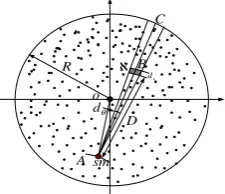
II. NETWORK MODEL AND PROBLEM DESCRIPTION Network architecture model: we apply the module similar with reference [6, 7], a typical wireless sensor network for cyclical data collection, a circle with radius of R, see Figure 2. In this network, there are

n

nodes,

{

N

₀,

N

₁,

N

₂,

N

₃,…

N

n},

N

0stands for sink and it can

move throughout the network, others represent work nodes and cannot move after initially deployed.

Communication range of nodes, is noted with

r

, the

difference from general sensor networks is that the transmission range is changeable, and nodes automatically adjust its communication range based on the distance between two nodes, for example, Berkeley Motes node has 100 transmission levels [6, 10]. Each work node will sense data in each cycle. We use the mature shortest path protocol for collecting data [11] and sending them to sink with multi-hop [11, 12].

θ

d ℵ

x

d

R

sm D

B

A o

C

Figure 2. Network computing model

Energy consumption model: We use typical energy consumption model, the cost of moving mobile sink is calculated according to formula 1 , cost for sending data is calculated according to formula 2, cost for receiving data see formula 3, specific details can be found in literature [5].

e k s sE

E_sin ( )= (1)

2

d

l

lE

E

_member

=

_elec

+

ε

_fs ifd <d₀ (2)

4 d l lE

E_member = _elec+

ε

_amp ifd >d₀

elec Rx l lE

E ()= (3) The cost for sending

l

bit of data can refer to 2.

elec

E

stands for the energy loss of firing circuit. If the transmission distance is less than the threshold

d

₀, power amplifier loss is based on free-space model; when the transmission distance is greater than or equal to the threshold value, it uses of multi-path attenuation model.

fs

ε

,

ε

amp represent the power for these two models’

amplification respectively. Energy for receiving

l

bit of

data refers to formula 3. In this paper, the above specific parameters come from the literature [5].

Problem Description: For a given mobile sensor networks shown in Figure 2, the problem can be described as: how to choose the anchors of mobile sink to maximize the network lifetime. Here we term the rounds of data collection till the first node die as the network lifetime [5, 10].

Ⅲ_.ANALYSIS OF ENERGY CONSUMPTION

A. Data Load Computing

When the sink moves to an arbitrary location such as (

x

₀

,

y

₀), if it is able to calculate the data load of each

Therefore, this paper will compute data load for each sensor node when sink is located at arbitrary (

x

₀

,

y

₀).To

the best of our knowledge, this paper gives derivation of data load in the network. It is also the basis for sink strategy in this paper.

Theorem 1: Suppose the center of network be O (0,0), sink has moved to A(

x

₀,

y

₀), an optional sensor node B

at (

x

_b,

y

b), and the intersection point of AB extension

with the network border is (

x

_c,

y

c), then the data load

for B node is as follows:

Dx

t =1+{(a-1-

i

)

c

+

(

1)(

)

(

)

2

a i

− −

a i r

+

}/(

ir

+

c

) // if

D=

ir

+

c

|

i

∈

{0..

a

},

c

∈

{

b

..

r

} // data sent Dx

r ={(a-1-

i

)

c

+

(

1)(

)

(

)

2

a i

− −

a i r

+

}/(

ir

+

c

) // if

D=

ir

+

c

|

i

∈

{0..

a

},

c

∈

{

b

..

r

} //data receive (4) Dx

t =1+((a-

i

)

c

+

( 1 )( )

( )

2

i+ +a a i r−

)/(

ir

+

c

) // if

D=

ir

+

c

|

i

∈

{0..

a

},

c

∈

{0..

b

} //data send

Dx

r =((a-

i

)

c

+

( 1 )( )

( )

2

i+ +a a i r−

)/(

ir

+

c

) // if

D=

ir

+

c

|

i

∈

{0..a},

c

∈

{0..

b

} // data receive

Note:

R

₁=_|AC_|,

α

= ⎥⎦ ⎥ ⎢⎣ ⎢

r R_{1 ,}

1

R

=

α

r

+

b

|

b

≤

r

.

D = |AB| =

ir

+

c

|

i

∈

{0..

α

},

i

= ⎥⎦ ⎥ ⎢⎣ ⎢ r

D _,

_c

_=D−ir,

_c

_∈

_{0..

_r

_}.

|

|

AC

=

(

x

c

−

x

₀

)

2

+

(

y

c

−

y

₀

)

2 ,

|

|AB =

(

x

b

−

x

₀

)

2

+

(

y

b

−

y

₀

)

2 .

Proof: This paper applies the shortest path routing

protocol to transmit data to sink through multi-hop. For an arbitrarily node

B

(

x

b

,

y

b) ,see Figure 2, C represents

intersection point of AB extension with the network border, the data load for B is the amount of data whose distance from B is integer multiple of

r

on line BC. First,

we calculate the coordinates of C (

x

c

,

y

c).

Equation of line AB: _{0 0}

0

0_{(x x ) y}

x x y y y b

b − +

− −

=

(5)

Equation of the circle:

x

2

+

y

2

=

R

2 (6)

Formula 5 can be simplified

as: _{0 0}

0

0_{(x x ) y}

x x y y y b

b − +

− − = = 0 0 0 0 0

0 _{x y}

x x y y x x x y y b b b b + − − − − −

Let

g

1= 0 0

x

x

y

y

b b

−

−

_, 2

g

= _{0 0}

0

0 _{x y}

x x y y b b ₊ − −

− =

y

₀-

g

₁

x

₀

2 1

x

g

g

y

=

+

, we can work out (

x

c

,

y

c) by substituting

it in formula (6):

0 2

) 1

( 2 2

2 2 1 2 2

1 + + − =

+g x g g x g R

Solving the coordinates of C can be divided into several situations as follows:

First: when

x

(

i

)

≠

x

₀

coordinates of C is as follow:

) 1 ( 2 ) )( 1 ( 4 ) 2 ( 2 2 1 2 2 2 2 1 2 2 1 2 1 g R g g g g g g x_c + − + − ± − = c

y

=

g

₁

) 1 ( 2 ) )( 1 ( 4 ) 2 ( 2 2 1 2 2 2 2 1 2 2 1 2 1 g R g g g g g g + − + − ± − ₊ 2

g

Note:

g

₁=

0 0

x

x

y

y

b b

−

−

_, 2

g

= _{0 0}

0 0

_x

_y

x

x

y

y

b b

+

−

−

−

if

x

_b

<

x

₀

then

) 1 ( 2 ) )( 1 ( 4 ) 2 ( 2 2 1 2 2 2 2 1 2 2 1 2 1 g R g g g g g g xc + − + − − − = c

y

=

g

₁

) 1 ( 2 ) )( 1 ( 4 ) 2 ( 2 2 1 2 2 2 2 1 2 2 1 2 1 g R g g g g g g + − + − − − ₊ 2

g

if

x

b

>

x

₀

then

) 1 ( 2 ) )( 1 ( 4 ) 2 ( 2 2 1 2 2 2 2 1 2 2 1 2 1 g R g g g g g g xc + − + − + − = c

y

=

g

₁

) 1 ( 2 ) )( 1 ( 4 ) 2 ( 2 2 1 2 2 2 2 1 2 2 1 2 1 g R g g g g g g + − + − + − ₊ 2

g

Second: when

x

_b

=

x

₀

if

y

_b

=

y

₀

then

this is the sink itself, no data

needs to be sent

if

y

b

≠

y

₀

then

x

c

=

x

0

2 2

2 _{y R}

x_c + _c =

if

y

_b

>

y

₀

then

y

c=

2 2

c

x

R −

if

y

_b

<

y

₀

then

y

c

=-2 2

c

x

R −

According to coordinate of C, the length of line AC is: |

|AC =

(

x

_c

−

x

₀

)

2

+

(

y

_c

−

y

₀

)

2

the length of line AB is: |

|AB = (x_b−x₀)2+(y_b−y₀)2 .

Let:R₁=|AC|,

α

= ⎥⎦ ⎥ ⎢⎣ ⎢

r R_{1 ,}

1

R =

α

r

+

b

|

b

≤

r

.

D = | AB| =

ir

+

c

|

i

∈

{0..

α

},

i

=

⎥⎦ ⎥ ⎢⎣ ⎢ r

D _,

_c

_=D−ir,

_c

_∈

_{0..

_r

_}.

Data load of B is calculated as follows. Its distance from sink is: D=|AB|=

ir

+

c

|

i

∈

{0..a},

x

∈

{0..

b

}.

Then check sector area

ℵ

with angle of

d

θ

, width of

dx

(See figure 2).The dimensions of this area is

this ring is:

ρ

Ddθdx .If it is located in the {

ir

..

ir

+b}|i

∈

{0..

a

}th ring,that is to say, the location

is :D=

ir

+

c

|

i

∈

{0..

a

},

c

∈

{0..

b

}, then data load of

ℵ

is:

It is responsible to forward all the remote data in sector area whose width is

dx

and is integer multiple of

r

away

from

ℵ

. The dimension of these areas can be computed as:

θ

d

((

i

+1)

r

+

c

)

dx

+

d

θ

((

i

+2)

r

+

c

)

dx

+

θ

d ((

i

+3)

r

+

c

)

dx

+…

d

θ

(a

r

+

c

)

dx

=

d

θ

dx

((a-

i

)

c

+(( 1 )( ) )

2

i+ +a a i r− )

This is the dimension of area

ℵ

is responsible to forward data. Then data load of

ℵ

is:

θ

d

dx

((a-

i

)

c

+

(

( 1

)(

)

)

2

i

+ +

a a i r

−

)

ρ

.

Data sent is: {(

d

_θ

dx

((a-

i

)

c

+

( 1 )( )

( )

2

i+ +a a i r− ₎₊

_θ

d

(

ir

+

c

)

dx

}

ρ

.

It can be assumed that the data load is uniformly shared by each node in a very small region. Then data load of each node is:

θ

d dx((

a

-

i

)

c

+₍( 1 )( ) ₎

2

i+ +a a i r− ₎

_ρ

_{/ θ}

d (

ir

+

c

)

dx

ρ

=((

a

-

i

)

c

+ ( 1₍ )( ) ₎

2

i+ +a a i r− _)/(

ir

+

c

).

Data sent

is:{(dθ

dx

(a

c

+ (1( ) )

2 a ar

+ _{)+dθ (}

_ir

₊

_c

₎

_dx

_}

_ρ

_/

θ

d

(

ir

+

c

)

dx

}

ρ

=1+((

a

-

i

)

c

+

( 1 )( )

( )

2

i+ +a a i r− _)/(

ir

+

c

)

If D=

ir

+

c

|

i

∈

{0..a},

c

∈

{b..

r

} is located in the

{

ir

+

b

,

ir

+

r

}th ring data load of

ℵ

can be computed as following:

It is responsible to forward all the remote data in sector area whose width is

dx

and is integer multiple of

r

away

from

ℵ

. The dimension of these areas can be computed as:

θ

d

((

i

+1)

r

+

c

)

dx

+

d

θ

((

i

+2)

r

+

c

)

dx

+

d

θ

((

i

+3)

r

+

c

)

dx

+…

d

θ

((a-1)

r

+

c

)

dx

=

d

θ

dx

((

a

-

i

-1)

c

+(( 1)( ) )

2

a i− − a i r+ )

Then data received by

ℵ

is:

θ

d

dx

((

a

-

i

-1)

c

+ (( 1)( ) )

2

a i− − a i r+ ₎

_ρ

_.

Data sent:

{(dθ

dx

((

a

-

i

-1)

c

+ ₍( 1)( ) ₎

2

a i− − a i r+ ₎

+

d

θ

c dx

}

ρ

It can be assumed that the data load is uniformly shared by each node in a very small region. Then received data of each node is:

{(

a

-1-

i

)

c

+

(

(

1)(

)

)

2

a i

− −

a i r

+

}/(

ir

+

c

).

Data sent is:

1+ {(

a

-1-

i

)

c

+ (₍ 1)( ) ₎

2

a i− − a i r+ _}/(

_ir

₊

_c

₎

B. Computing Node Energy Consumption

Corollary 1: Note the transmission range

r

with

f

_ri

(

x

)

,sink has moved to A(

x

₀

,

y

₀),an arbitrary

node B(

x

b

,

y

b),then the energy consumption of node B is:

) (x fi

r = Dr

×

Eelec+ Dt

×

Eelec+ Dt

×

ε

fs 2

x

if x<d₀ and i=0 )

(x

f_ri = Dr

×

E

elec+ Dt

×

Eelec+ Dt

×

ε

amp 4

x

if

x

≥

d

₀ and i=0 (7) )

(x

f_ri = Dr

×

Eelec+ Dt

×

Eelec+ Dt

×

ε

fs 2

r

if

r

<

d

₀ and

i

≠

0

)

(

x

f

_ri = Dr

×

Eelec+ Dt

×

Eelec+ Dt

×

ε

amp 4

r

if

r

≥

d

₀ and

i

≠

0

Proof: According to Theorem 1, the amount of

received data of nodes D=

ir

+

x

away from the sink is Dr, the amount of sent data is Dt=Dr+1.Substituting them in energy formula 1 and 2 will lead to Corollary 1.

Based on Theorem 1 and Corollary 1, Figure 3 shows the energy consumption under different sink locations and different

r

. As we can be seen from the figure, the

energy consumption of mobile sink is very complex. So it requires careful planning for moving sink.

(A) r=80, sink(350,0) (B)r=150, sink(0,0)

(C)150, sink(350,350) (D)r=150, sink(-350,-350) Figure 3. Energy consumption of network (R = 500)

algorithm to compute the movement of mobile sink. The central idea of the algorithm is:

First of all, we can obtain the network lifetime as rounds under optimal parameters when sink is located in the center. It is obvious that the network life will not be worse than rounds regardless of the mobile sink strategy. Sink moving along the circle trajectory has proven to be the best. If sink only collects data for one round at each anchor, the number of anchor is equal to the network life. If we can calculate the largest life of each trajectory, then parameters allows the largest lifetime is the result. In this paper the idea of the heuristic algorithm is: For each mobile trajectory (trajectory will be divided into discrete value in accordance with the application requirements) compute the largest network lifetime under each transmission radius as the r energy, then the maximum of r energy is the result.

Method for calculating is: set the current track radius as

Rm

, transmission range r, uniformly choose rounds node on current track, rounds is the best lifetime under optimal parameters when sink is located in the center. Sink conduct one round of data collection at each anchor. If the largest energy consumption is greater than the initial energy of nodes, it indicates no better lifetime of the network can be obtained under such r and

Rm

settings. Select the next transmission level and continue testing, if the largest energy consumption is less than the initial energy of nodes, it indicates better lifetime can be obtained under such r and

Rm

values. Algorithm will

seek the next stop and conduct a new round of data collection. If the largest energy consumption is less than the initial energy, then the largest network lifetime rounds = rounds +1, then algorithm continues to calculate the next stop. Repeat the above process until the largest energy consumption is not less than the initial energy of nodes, and then choose the next

r

, to continue testing until all

r

are tried, then we get the maximum network

lifetime under trajectory Rm. Repeating the process can obtain lifetime under different

Rm

trajectory in order to

get the greatest life of the whole network. Algorithm 1 gives the description of optimizing mobile sink.

algorithm 1：

Sink-Move_optimal(R, rbest, rounds,Rm) //pausing anchors for sink

1: compute lifetime rounds when sink static in centre //compute the lifetime when sink is located at the center of network

2: Rtj = R; //the initial track is on the circumference 3: while Rtj>0;

4: r= rmin 5: while r<rmax

6: Compute_xy(rounds, Rtraj, xy(n) ) //caculate the pausing ahchor rounds

7: trajectory_Energy_compute(Rtj, r, xy(n), E(m,n))

//compute the energy consumption of the network 8: max_energy =max(E(m,n)) //get the location for largest energy consumption

9: if max_energy>Einit //lifetime under current parameters is less than rounds stop considering these parameters

10: r=next(r) 11: break; 12: end

13: while max_energy<Einit

14: Compute_nextxy(rounds, Rtraj, xy(n+1) ) //energy left, sink move to next anchor abd conduct new data collection

15: compute_energy(R,x(n+1),y(n+1),r,energy(m,n) ) //add the energy of ne round data collection

16: E(m,n)= E(m,n)+ energy(m,n) //energy consumption for data collection

17: max_energy= max(E(m,n)) 18: if max_energy<Einit

19: rounds = rounds +1 //this is the current maximum lifetime rounds

20: rbest=r // this is the current best r 21: Rm=Rtfj // this is the current best Rm 22: End if

23: end do

24: r=next(r) //try next r level for lifetime incensement

25: end do //end (4)

26: Rtj= Rtj-rtj // move track inside, try next

Rm

level for lifetime incensement

27: end do

Algorithm explanation: Compute_xy (rounds, Rtraj, xy(rounds)) is to get the rounds docking points on the trajectory of Rtraj, all the points are stored in xy(n) vector, the locations are requested to be evenly distributed on the trajectory, and this can be implemented by algorithm 2. Compute_nextxy (rounds, Rtraj, xy (rounds +1)) is the function for adding a new docking point to the already rounds points on the trajectory, the generated points are uniform and symmetric, due to space limitations, we omit it here. The complexity of the algorithm is |R| * |r| * m * n, of which |R| is the number of track, |r| is the number of node transmission level, m * n is the number of grid after meshing the network. |r| is affected by the physical characteristics of the network. Other parameters are relevant with accuracy of actual application. If the application needs high precision, then number of grid and |R| increase and the algorithm complexity become higher and vice versa.

algorithm 2:

Compute_xy(rounds, Rtraj, xy(rounds ) ) //compute the rounds anchors

1: i=1

2: Do While (i <= rounds) 3: x = Rtraj * Sin(aa) 4: y = Rtraj * Cos(aa) 5: xy(i)=(x,y) 6: end do

V.PERFORMANCE ANALYSIS AND EXPERIMENTAL RESULTS COMPARISON

which is open source, component-based and modular for large network and has been widely recognized by the academic community [13]. Experimental parameters are shown at table 1 from the literature [5], if there is no special note.

A. Mobile Sink Network Performance Analysis and Experimental Comparison

LUO [7] claims that the optimal mobile trajectory is along the circle. We will justify the assertion and analyze the performance of sink on different route through theoretical and experimental verification. The main parameters of first scenes are as follows: Network radius

R

= 500m; the number of anchor is 20; the number of

nodes is 3000. It is easy to meet the conditions of 20 anchors in some applications. For example: Network radius

R

= 500m, each node generate 100bits of data in

each cycle, sink conducts 100 round of data gathering for each anchor point. we can get 20 anchors and life expectancy of the network is about 2000.

Figure 4 shows the theoretical calculated value based on Theorem 1 and Corollary 1. The experimental results show that energy cost for

R

m=400m is less than that of

m

R

=500m, this indicates the circumference is not

necessarily the best migrating route, and it is determined by real application.

(A)R=500,Rm=500 r=85, anchors=20 max energy=50597 (B)Rm=400 max energy=45749

(C) Rm=300 max energy= 46619

Figure 4 Optimal network lifetime when sink track is in the circle (theoretical results)

(A)R=500,Rm=500 r=85, anchors=20, max energy=58692 (B)Rm=400 max energy=53068

(C) Rm=300 max energy=54078

Figure 5. Optimal network lifetime when sink track is in the circle (experimental results)

Figure 5 is experimental results under the same scene. The experimental results are accordant with theoretical results. The theoretical results are based on the assumption that nodes are evenly deployed. However, nodes are randomly deployed in the experimental network. In fact the nodes are usually unevenly distributed. Therefore, data load of particular nodes may be higher and the actual energy they spend is correspondently larger than theoretical calculation. In addition, the maximum energy cost is not as smooth and concentrated as the theoretical values. Instead, they are sporadic. This is because: nodes are discretely deployed, there are only 20 anchors in scene one, resulting in

unbalanced energy consumption among nodes. Figure 5 is formed by numerically interpolating energy consumption of discrete node, thus, there are a series of small protrusions in areas of high energy consumption. However, the difference between experimental and theoretical results is about 10%, which is in line with reality.

5 10 15 20

25000 30000 35000 40000 45000 50000

en

er

gy

c

ons

um

pt

ion

(N

J

)

rounds Rm=300 Rm=400 Rm=500 R=500

r=85 anchors=20

5 10 15 20

20000 30000 40000 50000 60000

energy

c

ons

um

pt

io

n (NJ

)

Round Rm=300 Rm=400 Rm=500

Figure 6. Maximum energy consumption under different trajectory (theoretical value, scene one)

Figure 7. Maximum energy consumption under different trajectory (experimental value, scene one)

Figure 6 shows the statistical chart of maximum energy consumption after each round of data collection .It can be seen from the chart that when sink moves along the circle, the maximum energy consumption after each round of data collection are all large. There is a cross between chart of

R

m=400m and

R

m=300m and the reason is:

based on Corollary 1, the maximum energy consumption of

R

m=300m is the smallest. So when the number of

rounds is few, the maximum energy consumption is smaller. when the number of rounds is many, the energy consumption of nodes near the network centers after each round is high, so its energy consumption grows faster and finally is even higher than that of

R

m=400m. Figure 7

shows experimental results, the overall trends and theoretical analysis are consistent.

0 50 100 150 200

0 10000 20000 30000 40000 50000

distance

en

er

gy co

nsu

m

p

ti

o

n

(N

J

)

R=500 r=85 anchors=20

Rm=500 Rm=400 Rm=300

0 20 40 60 80

0 10000 20000 30000 40000 50000 60000

ener

g

y

c

ons

um

pti

on(

NJ

)

distance R=500 r=85 anchors=20

Rm=500 Rm=400 Rm=300

Figure 8. Profiles of energy consumption under different track (theoretical value, scene one)

Figure 9. Profiles of energy consumption under different track (experimental value, scene one)

generated by interpolation. If the selected straight line do not pass through the node with maximum energy cost, energy consumption of nodes on the trajectory is not necessarily the highest. In sum, The overall trend in Figure 9 is accordant with the theoretical results.

(A)R=500,r=85,Rm=500,rounds=100 max energy=157100 (B)Rm=400 max energy=170000

(C)Rm=300 max energy=191970

Figure 10. Optimal network lifetime when sink track is in the circle (theoretical result)

Figure 10 shows the energy consumption when sink trajectory respectively as

R

m =500m,400m,300m and

100 anchors, sink gathers data for one round at each pausing anchor. As can be seen from the chart, when the sink is on the circular trajectory of the mobile network energy consumption of the network is the minimum and the network lifetime is the largest. Figure 11 shows the corresponding experimental results. When the number of the anchor increases, the experimental results get closer to the theoretical results. Although the experimental results of energy consumption is larger than the ideal theoretical calculation, but the difference between them is less than 10%, so it is in line with the theoretical calculation.

(A) R=500,r=85,Rm=500,rounds=100 max energy=165390 (B)Rm=400 max energy=185440

(C)Rm=300 max energy=209664

Figure 11. Optimal network lifetime when sink track is in the circle (experimental result)

Figure 11 shows the maximum energy consumption after each round of data gathering. The result shows that at the beginning of data collection, the smaller

R

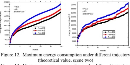
mis, the

smaller maximum energy consumption and total energy consumption will be. However, with the number of round exceeding certain degrees, energy dissipation rate of node in the middle of the network become rapid when sink get closer to the center of the network. At this time, energy consumption is lower when sink moves along the circumference. Here we get maximum energy expenditure shown in Figure 12. Figure 13 shows the experimental result which is in line with the analysis.

0 20 40 60 80 100

20000 40000 60000 80000 100000 120000 140000 160000 180000 200000

en

er

g

y

c

o

ns

um

p

tio

n(

N

J

)

rounds Rm=500 Rm=400 Rm=300 R=500

r=85 anchors=100

0 20 40 60 80 100

0 20000 40000 60000 80000 100000 120000 140000 160000 180000 200000

R=500 r=85 anchors=100

e

nerg

y

co

nsump

ti

on(N

J

)

rounds Rm=500 Rm=400 Rm=300

Figure 12. Maximum energy consumption under different trajectory (theoretical value, scene two)

Figure 13. Maximum energy consumption under different trajectory (experimental value, scene two)

B. Net Work Performance Comparison with Existing Mobile Sink Strategy

Next, we compare and analyze the efficiency of our mobile sink algorithm through experiments. Strategies discussed here include: 1) static sink [3]; 2) sink moves along the fixed circumference [7]; 3) Strategy proposed in this paper. We were referred to these three respectively as A, B and C strategy.

In order to fully contrast the effectiveness of experiment, all the algorithms should under the circumstances of optimal parameters. If only random settings of the parameters are compared, the comparison may be between the optimal performances of our algorithm with others’ non-optimal state, and then the result is unconvincing. We first analyze the optimal parameters for static sink network.

The life span of the network depends on the lifetime of those nodes consuming the highest energy. Therefore, in order to prolong the life expectancy, measures have to be taken to minimize the energy cost of nodes that dissipate the most energy. This section analyzes how to choose a transmission range to minimize the maximum energy consumption among nodes in static sink network, which is to achieve longest life span.

will become higher. This indicates mobile sink network is much better than static sink network.

0 20 40 60 80 100 120 140

0 200000 400000 600000 800000 1000000 1200000 1400000

staic sink

E

ner

gy

c

ons

um

pt

ion (NJ

)

rounds r=85,Rm=500 r=85,static sink r=170,static sink

the best staic sink

move sink

0 20 40 60 80 100 120 140

0 500000 1000000 1500000 2000000

static sink

E

nergy

consum

ption (N

J

)

rounds r=85 Rm=500 r=85,static sink r=170,static sink

move sink best static sink

(A) Theoretical results (B) Experimental results Figure 14. Energy consumption of different strategies (Scene three)

0 20 40 60 80 100 120 140 160

0 200000 400000 600000 800000 1000000 1200000

staic sink

move sink Rm=500

ene

rg

y

c

ons

um

pt

io

n (N

J

)

rounds Rm=350,r=85 Rm=500,r=85 static,r=170

move sink Rm=350

0 20 40 60 80 100 120 140 160 0

500000 1000000 1500000

Ener

gy

c

ons

umpt

ion (

N

J

)

rounds Rm=350,r=85 Rm=500,r=85 static,r=170

move sink ,Rm=350 move sink Rm=500

static sink

(A) Theoretical results (B) Experimental results Figure 15. contrast between static sink, mobile sink (along circle)

(Scene four)

Figure 15 shows the experimental results in scene four: network radius R = 500m, 20 anchors, sink conducts eight rounds of data collection at each anchor. For strategy A it is equal to sink collecting data for 160 rounds at the center, and strategy B migrates along the circular ,strategy C , however, moves along the track of Rm = 350m. The comparing chart between theory and experiment is shown in Figure 15. The strategy proposed in this paper, performs better than the other two strategies.

CONCLUSION AND DISCUSSION

The main contribution of this paper are: 1) presents a method to accurately calculate energy expenditure of the network when sink is located anywhere; 2) proposes a preferable off-line centralized mobile sink algorithms which can achieve better balanced energy consumption; In experiment section, we analyze the factors that affect network life in detail. The conclusion is of more general significance. As far as we know, there is no similar detailed analysis as in this article at present.

Although this article can present a more precise calculation of the energy consumption of the network, but the complexity of both of the centralized mobile algorithm and distributed mobile algorithm is still relatively large. Although we can calculate through unlimited sink energy, reducing the complexity of algorithm is worth further study.

ACKNOWLEDGMENT

This work was supported by China Postdoctoral Science Foundation 2012M511756

REFERENCES

[1] Wei Wang, Vikram Srinivasan, and Kee-Chaing Chua.

Extending the lifetime of wireless sensor networks through mobile relays, IEEE/ACM Transactions on Networking, 2008,16(5):1108-1120.

[2] Ioannis Chatzigiannakis, Athanasios Kinalis,Sotiris

Nikolets. Efficient data propagation strategies in wireless sensor networks using a single mobile sink, Computer Communications ,2008, 31(2):896–914.

[3] Anfeng Liu, Xin Jin, Guohua Cui, Zhigang Chen.

Deployment Guidelines for Achieving Maximal Lifetime and Avoiding Energy Holes in Sensor Network, Information Sciences, 2013, 230:197–226.

[4] Olariu S, Stojmenovic I. Design guidelines for maximizing

lifetime and avoiding energy holes in sensor networks wit h uniform distribution and uniform reporting .Proceedings of the IEEE INFOCOM. Barcelona , Spain , 2006 : 1-12

[5] Anfeng Liu, Zhongming Zheng, Chao Zhang, Zhigang

Chen, and Xuemin (Sherman) Shen. Secure and Energy-Efficient Disjoint Multi-Path Routing for WSNs, IEEE Transactions on Vehicular Technology, 2012, 61(7):3255-3265.

[6] Hossain A, Chakrabarti S, Biswas P K. Equal energy

dissipation in wireless image sensor network: A solution to energy-hole problem. Computers & Electrical Engineering, 2013, 39(6):1789-1799.

[7] Luo J, Hubaux J P. Joint sink mobility and routing to

maximize the lifetime of wireless sensor networks: the case of constrained mobility[J]. IEEE/ACM Transactions on Networking, 2010, 18(3): 871-884.

[8] Ming Ma, Yuanyuan Yang.SenCar: An Energy-Efficient

Data Gathering Mechanism for Large-Scale Multihop Sensor Networks, IEEE Transactions on Parallel and Distributed Systems, 2007,18(10):1476-1488.

[9] Mirela Marta, Mihaela Cardei. Improved sensor network

lifetime with multiple mobile sinks,Pervasive and Mobile Computing, 2009, 5(5):542–555.

[10]Jian Li, Prasant Mohapatra. Analytical modeling and

mitigation techniques for the energy hole problem in sensor networks[J],Pervasive and Mobile Computing, 2007,3(3):233-25

[11]EKICI E, GU Y, BOZDAG D. Mobility-based

communication in wireless sensor networks. IEEE Communications Magazine, 2006,44(7): 56-62.

[12]C. Intanagonwiwat, R. Govindan, D. Estrin, J. Heidemann,

and F. Silva, Directed diffusion for wireless sensor

networking, IEEE/ACM Trans .on Networking,

2003,11(1):2–16.

[13]Varga A. The OMNET + + Discrete Event Simulation