Map Matching Algorithm: Trajectory and Sequential Map Analysis on Road Network

Map Matching Algorithm: Trajectory and Sequential

Map Analysis on Road Network

Kanta Prasad Sharma

, Ramesh C. Poonia

, Raghvendra Kumar

, Surendra Sunda

,

and Dac-Nhuong Le

1_{Amity Institute of Information Technology, Amity University, Rajasthan, India} 2_{Department of Computer Science and Engineering, LNCT College, Jabalpur, India} 3_{Indian Space Research Organization, Ahmedabad, India}

4_{Faculty of Information Technology, Haiphong University, Haiphong, Vietnam}

Abstract

The Global Positioning System (GPS) tracking data is essential for sensor data sources. It plays an important role for various systems like Traffic assessment and Prediction, routing and navigation, Fleet management etc. Trajectory data accuracy is key factor for sampling based vehicle movement using existing GPS alerting systems. GPS navigation process is not reliable because of weak signaling transmission, weather scenario , specially, tall buildings area and drass sectors in Indian scenario. Map matching finding a path between available points on the active road segment, enhance road data accuracy through minimize frechet distance for future purpose. Therefore, accurate road data, become necessary for fast map matching outcomes. This work provides to locate the frechet distance on available free space for accurate path finding. This work also contributes to measuring frechet distance, trajectory data error estimation and finding free space surface on road network with sequential map computational method.

Keywords: Weak Frechet Distance, Error Aware, Map Matching, Trajectory Data, Adaptive Clipping, Free Surface Area

Received on 02 September 2018; accepted on 19 November 2018; published on 29 November 2018

Copyright © 2018 Kanta Prasad Sharma et al., licensed to EAI. This is an open access article distributed under the terms of the Creative Commons Attribution license (http://creativecommons.org/licenses/by/3.0/), which permitsunlimiteduse,distributionandreproductioninanymediumsolongastheoriginalworkisproperlycited.

doi:10.4108/eai.29-11-2018.155999

1. Introduction

Wireless sensor are very helpful for environment mon-itoring and communication process; researchers face challenges like computational constraints, link fail-ure, fault tolerance for coverage network which would improve with wireless sensor coverage performance and next generation sensor technologies is necessary for mobile communication systems which will helpful on high speed mobility and tracking services [1]. Global Position System (GPS) receivers are unified into vari-ous systems like Navigation system, Vehicle telemetric system, Intelligent Transport System (ITS), Smartphone etc. GPS services are not appropriate for real time navigation on the road network especially in drass

∗

Corresponding author. Email:[email protected]

sectors, high forestry sectors and tall building areas in Indian scenario. This era GPS users needs appropriate navigation approach without any tracking pitfalls. Map matching concept is useful for position finding on road network [2]. GPS receiver data is very necessary for position observing on digital road map. Navigation applications seriously work for accurate and reliable position sampling, analysis using sophisticated map matching algorithms, which result are not reliable due to available trajectory data quality.

This paper exploits GPS tracking trajectory data errors to pare down on the road network, presumably in the right tracking approach for high accuracy using fast map matching algorithm and adaptive clipping algorithm, which compute approximate real path between nearest road polygon’s circumferences. GPS trajectory data errors are finding; and reduce by computing frechet distance, between active surfaces of polygon circumferences [3]. Existing Adaptive Clipping algorithms provide local and global map

Research Article

EAI Endorsed Transactions

matching approach using Strong Frechet distance. Weak frechet distance is very important for local mapping approach; adaptive clipping approach neglect weak frechet distance for large network due to running time, storage complexity [4]. We also analysis output sensitive variant for weak frechet map using error-aware selection strategies for reliable navigation on curve polygon circumferences on road network. Trajectory Data- trajectory data is vehicle moving real time information like latitude, longitude, height, velocity, starting moment position, ending position elapsed time, etc, [5] which can easily collected using techniques such as Floating Car Data from many sources with appropriate file formats (OSM , XML files). Newson & Krumm [6] provides sophisticated map matching results based on available trajectory data, for real time position mapping on Google digital map which are not reliable for mobility time interval.

To address the challenges of map matching from noisy, low- frequency sampled trajectory data. Let we consider the large urban road network with part of different characteristic data. To compute smooth and optimized map between starting and ending moving points. The adopted approach; explore vehicle trajectories to analyzed segment and reconstruct the underline movements of network. This approach allows us to analysis input data set into groups of homogenous trajectory data and delay network.

The main contribution of this work focus on Proposed sequential map matching algorithm, Proposed vehicle location tracking algorithm, it provide optimized road network, based on original input data and threshold values, This work introduce, proximity turn sampled based algorithm for similar turns analysis on the road network and useful for create intersection nodes on available trajectory data [6]. Focus on optimized results using real data set according our research scenario to show the performance of proposed methods outperformance the current state of art.

This paper introduces, map matching issues and algorithms including optimum outcomes. Section 2 provides background details and Frechet Distance and issues are discuss in Section 3. Section 4 surmised Existing Map Matching Issues and in Section 5, we will propose Sequential Map Matching Algorithm. Section 6 Provides Results and Discussion and finally we surmised conclusion in section 7.

2. Background

Map matching algorithms are use full for trajectory data process and exact location finding on appropriate time period. Adaptive Map Matching Algorithms works as Incremental and Global Map Matching Algorithm for vehicle location tracing in different road situations. Quddus, et.al [7] provides, an incremental algorithm

principle based on greedy strategy with historical mapping results, for active surface area in road network similarly Goh C. Y et.al [8] & He Z. C et.al [9] provides, incremental algorithm with sliding window and recursive principle; Sliding window divide trajectory data into the smallest points, for sequential processing when sliding window size continuously updated with segment points is large, algorithm provides optimal results.

Karagiorgou et.al [10] introduces the look ahead method for delay analysis between each segment points. Yin et.al [11] proposed, a high quality map matching method for computing nearest point’s trajectory data; on active surface area of the road network which is indicates through a weighted graph, every weighted edges are decoding the distance between vehicles position for calculate shortest Path value using Dijkstra’s Algorithm.

Wenk.C et. al [12] introduce, an appropriate route-finding approach using road and geometric analysis for Point to point map matching approach or line segment tracking in different whether situation on road network. Mostly route tracking research is based on GPS trajectory [13] for vehicle’s variability which is more reliable than personal trajectory data collection approach Similarly, Chen. L, et.al [14] proposed, personal trajectory data collection approach which would face adequate challenges for example the diversity of trajectory data on each movement. Frechet distance is necessary parameter for accurate route finding between road networks. A global algorithm for finding all possible polygon circumferences (circular path) on appropriate velocity of vehicle [15].

The objective is to enhance the performance of global map matching algorithm for kinetic and precise point positioning for real time tracking.

3. Frechet Distance

Curve matrix space provide computed results between polygons inO(p×_q×_log2p×_{q) time wherepandqare}

curve polygon segments for example, suppose a man walking a dog in forward direction with continuous velocity where belt’s minimum distance (between man and dog) indicate strong frechet path on active segment length and weak frechet path indicate belt’s length [15]. Strong and weak path depend on belt’s variant, for example suppose distance ( >0) means, distance is fixed or not [27]. Alt H & Godau [16] provides a binary search method for curve circumference’s radius variants atdistance or >distance.

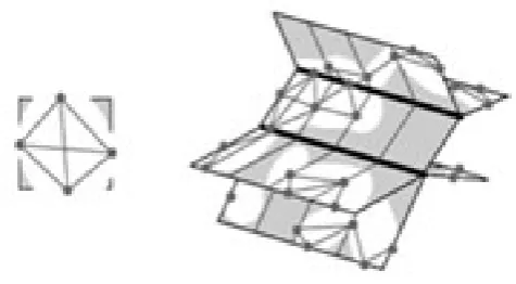
Figure 1. Road Network (left) and White surface (right)

4. Map Matching Issues with Algorithms

Map Matching is a used for continuous and smooth navigation process. Existing navigation systems are working on positional data such as longitude, latitude but, mostly systems are neglect altitude for route mapping approach on the horizontal surface; it becomes imbalance for sophisticated regions like ground road network, for example, hill station routes, rural region and tall building area. Map matching algorithms appropriate results are depend on trajectory data and digital map quality.

4.1. Problem

LetT = (Tn|n= 1,2, .., N) sequence ofN vertices of the road network.

Every point (Tn) identify necessary parameters like Longitude, Latitude, Speed and Time stamp respectively (Tn.Lon), (Tn.Lat), (Tn.v), (Tn.t).

Procedure for computing GPS points threshold [17], letT= time interval between vertices and GPS log point under a certain threshold:

∆t, T :P1→P2→P3→...→Pn (1) wherePi ∈L, means contains (latitude, longitude and time stamp) in range 0< pi+1.t−pi.t <(1≤n).

Segment. Let R is the mapping point on polyline

(Figure2) which indicates curve segments on the road. Number of nodes are lies on a line are indicate as (p1, p2, .., pm), where each node contain Longitude and Latitude where segments with

• Road width (r, w). • Speedlimit(r, v)

• Bi-direction travel [r, d∈_{T rue, False].}

Figure 2. GPS Trajectory

Digital map. Map is a combination of many segments (k) of a road network. It provides route and location of the vehicle. Let G={_rk|_{k= 1,2, k}}_{. The objective is}

to find out corresponding trajectory point (T) between segments (G).

4.2. Map matching algorithm

Map matching performance can enhance using some strategies such as graph optimization, error awareness with trajectory data, and result in the sensitive process using adaptive clipping technique.

Algorithm 1Turn and Segment Analysis

Input: Trajectory set (T) and speed categories (C) Output: A set of trajectory segment based on speed. BEGIN

Tsegm← ∅ ForTsegm∈T

For each (LJ ∈T)

U(Li)←median(U(LJ−w)), V(Tsegm)∈C

Tsegm←Tsegm∪Lg, C End for

End for ReturnTsegm END

Graph Optimization algorithm. A traditional approach of curve polygon’s frechet distance computation on variant frames inΘ(m, n) time duration, here m,nare curve polygon conditions where active points are search out using graph traveling technique [18]. GPS trajectory position complexity for shortest path computation between nearest active points on road segment inO(m×

nlog(m×_{m)) time and Θ(m}×_{n) space complexity for}

every shortest path < ∗

, where ∗

indicate optimal frechet distance andrepresent weak frechet distance.

White surface indicate active surface area for optimal path analysis, where every pair of vertices (v) connected by an edge (e) for a path (v, e).

Sensitiveness algorithm. An optimal shortest path is important for historical data on previous tracking graph. Hash table maintain historical information on

O(1) time for each entity similarly output sensitive algorithm requires O(k×_{logk) time, where K indicate}

required free space for every shortest path between start (e, p0) and end (f , pn) nodes, e and f are roads with p0 and pn position points. Sensitiveness method for shortest path finding with trajectory data refining process for upgrading map matching performance [19].

Error aware map matching. Real time tracking applica-tions services are not reliable due to GPS signal fre-quency and receiver performance which is causes of tracking in GPS restricted areas, tall buildings region, narrow streets, high drass sector in our scenario. One most causes of GPS error is signal reflection when trans-mitted on Satellite Based Augmentation System (SBAS) due to satellite’s health or weather circumstances.

The following Lemma encodes the observed tory properties for the road network for signal trajec-tory:

Lemma 1: The positive vehicle trajectory of the

verticesq1..qmin a road network that has encoded to the vertices trajectoryp1..pnincluding following properties

• Initial Stage:q(1)∈A(pi) • Final Stage:q(m)∈A(pi)

• Intersection:q1..qmfor IntersectA(pi) 1≤0≤n • Containment: ifq1∈A(pi) andqi+k ∈A(PJ+1) Proof:

• Starting vertexq1is belongs to active areaA(p1) in curve (polygon).

• Ending vertexqmis belongs to active areaA(pn) Each active vertex (n) must intersect on free space including regular moving position from start vertexpi and end vertex pi+1 with measurement errors means [q1∈A(pj) andqi+k ∈A(pj+1)].

Adaptive Clipping Algorithm. Adaptive Clipping algo-rithm working for localized map matching on weak frechet distance, for example, suppose trajectory edge between pi andpi+1 ispipi+1 on velocity (v) and sam-pling rate (r) with every pi in active area A(pi). On curve centerpi with radiusµor measurement error (µ) [20] and Dijkstra’s Shortest Path Finding algorithm is implementing on two conditions.

Condition 1. Dijkstra on free space graph, finding the shortest path between start (pi) to end (pi+1) vertices. Free space graph vertices (p1, e), (v, p1p2), (p1, e) here,

• vis vertex;

• eis edge for (AP1P12) [continuous changing radius of curve] and

• eis an edge forA(P2) [means Active region]. Condition 2. Dijkstra on (n−_{1 vertices) for all available}

vertices (pi, e), (v, pipi+1),pi+1, e) on free spaces graph, here,

• vis vertex;

• eis an edge inA(pipi+1) and

• eis an edge in A(pi+1)[(v, pipi+1)] for continuous moving position [12].

Now, we can filter GPS trajectory data (error free) for sensitive results on the continuous ways on the rod networks.

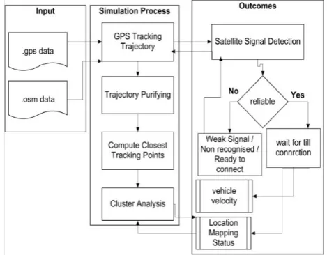
Figure 3. Methodology for GPS Signal detection Process onL2

Frequency Data

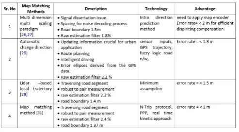
Table 1. Existing Map Matching Algorithms

5. Proposed Map Matching Approach for

Sequential Map

5.1. Bayes Approach

This approach provide periodic information with likehood [32]. When we, compute time difference parameter based on filtering algorithms upon trade of between accuracy and complexity. The Kalman filter algorithm [35, 37] is adopt for simplicity implementation, tractability and robustness [33].

5.2. Proposed Filter

To estimate the position of vehicle (VO) in fixed time interval, existing research work neglect the motion of vehicle [23]. Now, consider the focus on dynamic outputs, we adopt Bayesian filter for particle-tracking nodes position tracking.

X0(k) = [x0(k), y0(k), s0(k), h0(k)] (2) Here,

• x0(k), andy0(k) is vehicle position coordinates of timek.

• s0(k) is the vehicle speed (m/sec).

• h0(k) is consider as vehicle heading (in ration) form the x-axis to consider the direction and measure the positive angle [40].

The state space is consider based on

x0(k) =x0(k−1) +Ts0(k−1)cos(ho(k−1)) (3)

y0(k) =y0(k−1) +Ts0(k−1)sin(h0(k−1)) (4)

s0(k) =se0(k) +wk (5)

h0(k) =h0(k−_{1) +}eh+w_k (6) Here,

• T is time interval betweenk−_{1 andk(in seconds).}

• ∆_his estimated heating change route during each interval (1 sec).

• sk is estimated average speeds with in time interval when noise is define both heading and speed as Gaussian distance.

• wk is consider as normal distribution have zero mean variations and measure equation define by 2(k) for composite vector of timek.

To compute individual GPS position

p0(k) =p0− |s∝logkxa(k)−x0(k)kv0(k)| (7) Here,v0is vehicle position uncertainty.

e

xak= [exa,yea]

T ₍₈₎

Gaussian distribution with meanxaas the measure of GPS position and [xea,yea] measure GPS position based on k derivation time interval.

5.3. Map Information

In case, road map is available [22], then compute difference between road and no road area. The proposed computation method adopt open start map (osm) where each roads are linked by a single edge line without consider the width of road. We optimized the output based on 10 m road segment as input and road directions are consider as similar or opposite. This work keeps the highest value to select road site trajectory nodes.

5.4. Lane Level Map

The road map information is considering lane level data to scaling suitability between micro scale dense points, which are more suitable or reliable for intelligent vehicles location tracking. These dense points are more accurate without long delay [27]. The Map’s prototypes are utilized to cover 4 km in Ahmedabad & 2 km another network. The proposed sequential map-matching algorithm provides high quality outcomes.

Road Geometric Information. Polyline provides the geom-etry information of vehicle moving segment. The seg-ment is split into various subsets of segseg-ment with segment heads.

Road Lane Marking. Each lane having Meta data with respect to markings delimiting, Geometric description provides some extra information such as solid lines for tracked segment [28].

Road Lane/ Segment Connections. No real time accurate tracking/navigation information in terms of connection

The trajectory satisfies:

T(α) : [0,1]→_{xij (9)}

with

T(0) = (0,0)T (10) and

T(1) =xlocation, ylocation (11) The trajectory will initially- input by curvature. Now, need to analysis that some mapping M (Cartesian coordinates):

T (α)↔M_{ft(α, qt) =}

"

fx(α, qt)

fy(α, qt) #

(12)

f(α, qt) Indicate simulation model being t shown trisection andqare recursive parameters for process.

Consider the global reference frames, when need to re align location with the regional mapping trajectory at every time slot means

x_tr =pr_t = 0 (13) The simulation model can be simplified

xr_t+1= (∆_n+n), yt+1= 0 (14) Now, the updated local map (OSM-Open Street Map) to be consider with the vehicle location can be measured as [29] (∆n,∆φ) including associated uncertaintyσ∆.

The given matrix provides movements computation parameters

[xt+1, yt+1,1]t =T

−₁

[xt, yt,1]T (15) Here

T =        

cos(∆_φ) −_sin(∆_φ) ∆_n

sin(∆φ) cos(∆φ) 0

0 0 1

       

(16)

Suppose mapping is restrictMto be a linear function, the simulation parameters of the form

f(α, φ) =θA(α) (17) Now, the new coordinate parameters are [30]

xt+1=Txt=T f(α, qt) =TqtA(α) =QA(α) (18)

Qt+1=TqtA(α) (19) The frequency of this computation is much better than existing process shown in Table 2.

Table 2. GPS Raw Estimation information

5.5. Segment Fatching Approach

The proposed algorithm is categorized on hierarchy level, which are given below:

1. Map (.osm) data files are deploy for mapping the vehicle location according GPS sensor tracking trajectory- the velodyne H10Z-64 laser sensor used for evaluate sensor’s generated pit cloud

2. The Road generating algorithm provides road boundary’s information by vehicle sensor data then compute using RANSAC/ least- sequences approach for optimal trajectory point’s analysis.

3. Vehicle should be implement odometer sensors-to estimate local map updated information after vehicle movements

4. The reference trajectory utilized steer the vehicle for local maps using segment traversal approach.

Figure 4. Working Methodology for Road Analysis and Tracking Process

Here, we compute two important possibilities that are outcomes from the fact, which we are planning on the local road network. In the algorithm 2, step 1 indicate the GPS location which may be inaccurate that navigating precisely to related coordinate in step 2.

Algorithm 2. Road Analysis and Tracking Process

Input: Segment heads, road missing data, Odometer-calculated inputs. BEGIN

Step 1. Check current position of vehicle on road network while (current_possition ),osm_possition) do

Step 2. Check current GPS Position on purified Trajectory of road network. GPS input,purified trajectory input

Step 3. Simulate trajectory input/ receiver type or single type (PPP-Precise Point Position/STATIC/Dynamic) Step 4. End of outer while

Step 5. Compute new trajectory data based on GPS sensor input Step 6. Compute probabilistically force reference trajectory Step 7. End of outer while

END

Algorithm 3. Map Matching Vehicle Tracking Input:

- Global Position Data (.GPS) - Updated Road map data (.OSM)

Output: Estimate optimized path with tracking nodes and moving vehicle direction. BEGIN

Step 1. Get initial position and uncertainty from individual data. Step 2. Initialized trajectory frechet distance free space randomly.

Step 3. Measure moving object speed and continuously change segment head from initial to next. For eachsegmentdo

Compute sample speed error; Compute sample heading error;

Compute node displacement update state; End For

Step 4. Check map conditions

Minimized the node frechet distance; Check the curve type;

Manage historical moving nodes location; Step 5. Analyzed the position

Track real time GPS location (long, Lat);

Purify the uncertainty of signals using Gaussian probability mechanism ; Step 6. Check threshold

If (Sum (weight) < zero_threshold)then

Repeat Step 5; Else

Compute optimized weight; Compute optimized speed; End If

Step 7. To resampling threshold on the path

If sum(weight2 )<resampling thresholdthen

No need to lowest weight nodes; Else

Consider highest threshold nodes; End If

Step 8. Mapping Status Get optimized map;

Compute tracking nodes on map; Measure the velocity (speed); Step 9. Exit

Now, we consider the corresponding speed category to each segment. The nature of vehicle movement; it preserve the high degree of fragmentation and refining the data set unusable. When start the movement, velocity (speed) is consider low down due to intersection or other kinds of issues but, we adopt sliding window cross the trajectory and replacing the speed value of each segment based on median computation over a series of consecutive line segment (smooth head) value [35]. This approach will help us to avoid excessive fragmentation of trajectory due to short change in speed. The process highlighted some objectives:

• Every line segmentljon each trajecotryTstep 1. • The median speed is computed over a sliding

window of width (w)2 in step 2.

• All segments are assign to related classes with minimum and maximum speed computation step 5 and step 6.

6. Results and Discussion

We were trying to calculate precise position within any appropriate accuracy, need to input necessary information such as longitude, latitude, height and timestamp of the base station or GPS receiver position for reliable data collection on geodetic and ellipsoidal height.

Simulation tool: RTKLIB1_{is an open source program} package for standard and precise positioning with GNSS (Global Navigation Satellite Systems). RTKLIB consists of a portable program library and several APs (Application programs) utilizing the library. It supports standard and precise positioning algorithms with: GPS, GLONASS, Galileo , QZSS, BeiDou and SBAS

• It supports various positioning modes with GNSS for both real-time and post-processing: Single, DGPS/DGNSS, Kinematic, Static, Moving-Baseline, Fixed, PPP-Kinematic, PPP-Static and PPPâĂŘFixed.

• It supports many standard formats and protocols for GNSS: RINEX 2.1, 2.11, 2.12 OBS/NAV/GNAV/HNAV/LNAV/QNAV, RINEX 3.00 , 3.01, 3.02 OBS/NAV, RINEX 3.02 CLK, RTCM

• It supports several GNSS receivers’ proprietary messages: NovAtel: OEM4/V/6, OEM3, OEM-Star, Superstar II, Hemisphere: Eclipse, Cres-cent, u-blox: LEAâĂŘ4T/5T/6T, SkyTraq: S1315F, JAVAD/ GRIL/GREIS,

1_{www.rtklib.com/}

• It supports external communication via: Serial, TCP/IP, NTRIP, local log file (Record and playback) and FTP/HTTP (Automatic download).

• It provides many library functions and APIs (Application program interfaces)

Data Set: Give data set is deploying for location tracking simulation process. Here longitude, latitude indicate location of vehicle movements within fixed time interval and moving directions are indicate byX

andY respectively left and right direction. Table 3. Dataset information

Here, observation represents the variations on time intervals for moving direction as well as location on adopted open street map. The rapidly changes on the tracking node depend on the longitude and latitude values.

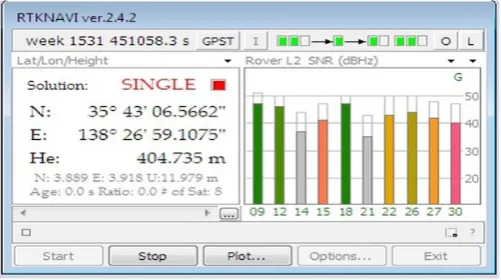
Figure 5. Solution status position on carrier phase L1

color bar where gray represents not used, orange means waiting for connection, deep green means connecting or running, light green means data active or processing, red indicate communication errors, deep pick upcoming activation status message.

After input observation, compute the position solution for GPST status or X/Y /Z means longitude, latitude and height component including ration factor of ambiguity validation in the figure because unreliable input data become causes of high level pitfalls such as position error, residual error.

In case, computing precise position onL1orL2carrier phase; results are not up to mark due to weak GPS signaling indicated in Figure.6.

Figure 6. PPP signal status on carrier phaseL1 In addition, when computing precise position points with high frequency carrier phase L5, GPS signals are not recognized for other input streamL5represented in Figure7.

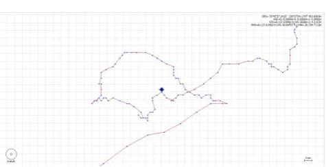
Figure 7. PPP signal status on carrier phaseL5 The road segment and traveling points are indicated in Figure8and technical summary is shown in Table 2.

Figure 8. Vehicle location movements on L2 frequency signals

7. Conclusion and Future Work

This work introduces a fast and accurate map matching algorithm and adaptive Clipping algorithm for all possible curves navigation with minimum weak frechet distance in local frechet space. We introduce map-matching issues with solution strategies for error awareness solution and provide mathematical exposure for process analysis. The proposed method raw estimation summary is providing in the given Table 2.

In addition to the future work, we would like to compute precise position for narrow streets, hill station routes, rural region and tall building area with GPS services on L1/L2 carrier phase signals or high quality frequencyL5carrier phase signals using another satellite system (IRNSS) which is helpful for precise navigation in our scenario.

References

[1] Shiv. K. Gupta & Ramesh. C, Poonia . A comparative study of mobile wireless networks , Oriental journal of computer science & technology, 4(2), 387-392, 2011. [2] Eriksson, J. et.al, The pothole patrol: using a mobile

sensor network for road surface monitoring , In Proceedings of the 6th international conference on Mobile systems, applications, and services, pp. 29-39, 2008.

[3] Alt, H., & Godau, M, Measuring the resemblance of polygonal curves , In Proceedings of the eighth annual symposium on Computational geometry, pp.102-109. [4] Brakatsoulas, S., et.al, On map-matching vehicle

track-ing data , In Proceedtrack-ings of the 31st international con-ference on Very large data bases, pp. 853-864, 2005. [5] Pfoser, D., et.al, Dynamic travel time provision for road

networks , In Proceedings of the 16th ACM SIGSPATIAL international conference on Advances in geographic information systems, pp. 68.2008

[7] Quddus, M. A., et.al, A general map matching algorithm for transport telematics applications.GPS solutions , Issue 7(3), pp. 157-167, 2003.

[8] Goh. C. Y.et.al, Online map-matching based on hidden markov model for real-time traffic sensing applications , In Intelligent Transportation Systems (ITSC) on 15th International IEE Conference, pp. 776-781,2012 [9] He, Z. C, et.al, On-line map-matching framework for

floating car data with low sampling rate in urban road networks , IET Intelligent Transport Systems, 7(4), 404-414, 2013.

[10] Karagiorgou, S. & Pfoser, D, On vehicle tracking data-based road network generation , In Proceedings of the 20th International Conference on Advances in Geographic Information Systems, pp.89-98, 2012. [11] Yin, H., & Wolfson., O, A weight-based map matching

method in moving objects databases , In Scientific and Statistical Database Management Proceedings on16th International Conference, pp. 437-438, 2004.

[12] Wenk, C., Salas, & Pfoser, D, Addressing the need for map-matching speed: Localizing global curve-matching algorithms In Scientific and Statistical Database Man-agement on 18th International Conference, pp. 379-388, 2006.

[13] Froehlich, J. & Krumm, J, .Route prediction from trip observations (No. 2008-01-0201), 2008.

[14] Chen, L., Lv, M, Ye Q. & Woodward, A personal route prediction system based on trajectory data mining , Information Sciences, 181(7), 1264-1284, 2011.

[15] Alt, H., & Godau, M, Computing the FrÃľchet distance between two polygonal curves , International Journal of Computational Geometry & Applications, 5 (2), 75-91, 2016.

[16] Alt, H., Knauer, C., Wenk, C, Comparison of distance measures for planar curves , Algorithmica, 38(1), 45-58, 2001.

[17] Lou, Y., et.al, Map matching for low sampling rate GPS trajectories , In Proceedings of the 17th ACM SIGSPATIA, international conference on advances in geographic information systems, pp. 352-361,2009. [18] Alt, H., Knauer., C., Wenk, C, .Matching polygonal

curves with respect to the FrÃľchet distance , In Annual Symposium on Theoretical Aspects of Computer Science, pp. 63-74, 2015.

[19] Chan., T., M, Optimal output-sensitive convex hull algorithms in two and three dimensions , Discrete & Computational Geometry, 16(4), 361-368, 2016. [20] Svarm, L., Enqvist, O. Oskarsson, M & Kahl, Accurate

localization and pose estimation for large 3d models , In Proceedings of the IEEE Conference on Computer Vision and Pattern Recognition, pp. 532-539, 2014.

[21] Agarwal, P. K., Avraham, R. B., Kaplan, H., & Sharir, M, Computing the discrete FrÃľchet distance in subquadratic time , SIAM Journal on Computing, 43(2), 429-449, 2015.

[22] Chen, B. Y.et.al, .Map-matching algorithm for large-scale low-frequency floating car data , International Journal of Geographical Information Science, 28(1), 22-38, 2004. [23] Dai, J. Ding Z. M., Xu, J. J, Context-Based Moving Object

Trajectory Uncertainty Reduction and Ranking in Road Network. Journal of Computer Science and Technology ,

31(1), 167-184, 2016.

[24] Encarnacion, I.V., et.al, RTKLIB-based GPS localization for multipath mitigation in ITS application , In Ubiq-uitous and Future Networks on Eighth International Conference, pp. 1077-1082 ,2016.

[25] Gheibi, A, Maheshwari, A., & Sack,J. , Minimizing Walking Length in Map Matching , In International Conference on Topics in Theoretical Computer Science, pp. 105-120 ,2015.

[26] Zhang, T., et.al, A trajectory-based map-matching sys-tem for the driving road identification in vehicle nav-igation systems , Journal of Intelligent Transportation Systems, 20(2), 162-177, 2016.

[27] Lucas, L. F., Rodrigues, N. M., Pagliari, C. L., da Silva, E. A., & de Faria, S. M., Recurrent pattern matching based stereo image coding using linear predictors , Multidimensional Systems and Signal Processing, 28(4), 1393-1416, 2017

[28] Yang, X., Tang, L., Stewart, K., Dong, Z., Zhang, X., & Li, Q., Automatic change detection in lane-level road networks using GPS trajectories , International Journal of Geographical Information Science, 32(3), 601-621, 2018.

[29] Gu, Y., Hsu, L. T., & Kamijo, S., Towards lane-level traffic monitoring in urban environment using precise probe vehicle data derived from three-dimensional map aided differential ,GNSS,2018

[30] Pepperell, E., Corke, P., & Milford, M., Routed roads: Probabilistic vision-based place recognition for changing conditions, split streets and varied viewpoints , The International Journal of Robotics Research, 35(9), 1057-1179, 2016.

[31] Lou, Y., Zhang, C., Zheng, Y., Xie, X., Wang, W., & Huang, Y. (2009, November). Map-matching for low-sampling-rate GPS trajectories. In Proceedings of the 17th ACM SIGSPATIAL international conference on advances in geographic information systems (pp. 352-361). ACM. [32] Hsueh, Y. L., & Chen, H. C. (2018). Map matching for

low-sampling-rate GPS trajectories by exploring real-time moving directions. Information Sciences, 433, 55-69.

[33] Ozdemir, E., Topcu, A. E., & Ozdemir, M. K. (2018). A hybrid HMM model for travel path inference with sparse GPS samples. Transportation, 45(1), 233-246.

[34] Zhang, Y., & He, Y. (2018, March). An advanced interactive-voting based map matching algorithm for low-sampling-rate GPS data. In Networking, Sensing and Control (ICNSC), 2018 IEEE 15th International Conference on (pp. 1-7). IEEE.

[35] Mozas-Calvache, A. T. (2018). Accuracy assessment of speed values calculated from GNSS tracks of roads obtained from VGI. Survey Review, 1-10.

[36] HÃďuçler, J., Stein, M., Seebacher, D., Janetzko, H., Schreck, T., & Keim, D. A. (2018). Visual Analysis of Urban Traffic Data based on Resolution and High-Dimensional Environmental Sensor Data. In EnvirVis 2018: Workshop on Visualisation in Environmental Sciences.

using RTKLIB. Cluster Computing, 1-9.

[38] Sharma, K. P., Poonia, R. C., & Sunda, S. (2017, December). Map matching approach for current location tracking on the road network. In Infocom Technologies and Unmanned Systems (Trends and Future Directions) (ICTUS), 2017 International Conference on (pp. 573-578). IEEE.

[39] SHARMA, K. P., POONIA, R. C., & SUNDA, S. (2018). Real Time Location Tracking Map Matching