Feature Recognition Using Basic Tools
1
Joy Gopal Goswami,
2Dr. Aditya Bihar Kandali
1,2Dept. of Electrical Engineering, Jorhat Engineering College, Assam, India
Abstract
Feature recognition is the most fundamental stage in most
real-world and scientific image processing applications. A large variety of detectors, that principally compute features at particular locations in an image or a region specified within it, have been developed. With the advent and passage of time, modifications and alterations to previous works, as well as new developments have greatly simplified feature recognition tasks, at the same time removing hurdles previously inherent with respect to recognition due to scale changes, illuminations, affine distortions etc. SIFT and SURF are the principal tools in use today, that are worth discussing.
Keywords
Harris Corner Detector, SIFT, SURF, Hessian Matrix
I. Introduction
Image correspondences between two images of the same scene are an important part in dealing with feature recognition problems,
which are mainly found in three stages:
Interest point detection at distinctive image locations (corners, 1.
blobs etc.).
Representation of the neighbourhood of interest points by a 2.
feature vector or descriptor.
Matching feature vectors or descriptors between different 3.
images.
Detectors used to find such correspondences need to be simple and accurate, while the descriptor used should be distinctive and of optimum dimensionality.
Most detectors and descriptors present [1,2,3,4] are devoid of the compromise between quality and speed. For the purpose of
this article, we discuss the two most widely used
detectors-cum-descriptors, SURF [5] and SIFT [2, 6], which promise to be more distinctive and repeatable than the others.
II. Background
Detectors can be of many types – some detect edges, others detect corners, while some others work directly upon the gray level
features, and some even go further on elucidating the effect of
gray level derivatives or similar mathematical parameters.
Harris and Stephens in their work [7] claim that the detector proposed by them has been found to satisfy the criteria proposed by Schmid et al. in a better fashion than others. However, the Harris detector fails to perform efficiently under large scale changes, barring which it gave geometrically stable interest points.
It basically uses the auto-correlation function for computing
locations where the signal changes in two dimensions and thus,
locates interest points, proving to be more efficient than “state-of-the-art” edge filters, like that of Canny’s [9], which cannot cope with junctions and corners and thus, cannot provide edge connectivity. By detecting both edges and corners in the image, a junction is obtained at those corners where edges meet. The local window considered in the image, as shown in Moravec’s work [10], is shifted by a small amount in various directions and
depending on the resulting average changes of image intensity, it is ascertained whether the window encompasses a flat region, an edge or a corner. Mathematically, the intensity change E produced by a shift (x, y) is
∑
+
+
−
=
v uy
x
I
v
y
u
x
I
v
u
w
y
x
E
, 2)
,
(
)
,
(
)
,
(
)
,
(
where, w specifies the image window; its value is unity within a specified rectangular region and zero, elsewhere.
Harris, however, incorporated appropriate corrective measures to overcome the problems encountered by the Moravec detector and
devised his corner detector, in the following way:
Performing an analytic expansion about the shift origin in 1.
order to cover all possible shifts of the local window. Using a smooth circular window (preferably Gaussian) to 2.
render the response free from noise, inherent on using a rectangular window.
Reformulating the corner measure to make use of the variation 3.
of E with the direction of the shift. Thus,
where M is a 2 X 2 symmetric matrix given by
∑
=
y y y x y x x x vu
I
I
I
I
I
I
I
I
v
u
w
M
(
,
)
,
The eigenvalues of M are proportional to the principal curvatures of
the local autocorrelation function and form a rotationally invariant
description of M. Depending on the principal curvatures, the type of windowed region can be ascertained.
If both curvatures pertaining to the two eigenvalues are small, 1.
the window encompasses a flat region.
If one curvature is high and the other low, the window can 2.
be said to encompass an edge.
If both the curvatures are high, a shift of the window in any 3.
direction results in an increase in E and indicates a corner.
Harris detectors are used to find corresponding features, or more appropriately corners, across two or more views. The elements to be matched are image patches of fixed sizes. The principal objective is then reduced to finding the best match amongst the patches between two or more images. However, all patches are not similar and distinctive, which creates problems in the detection process.
The local sum-of-squared-differences (SSD) approach is a better detector with respect to gray level derivative based detectors. The
self-similarity measure forms the foundation for a large class of
detectors, one amongst them being that of Harris and Stephens [7] – who computed a second derivative approximation of the SSD with respect to the shift. The resulting Hessian matrix consists of elements which are averaged over the entire image patch area.
=
Η
2 2However, second derivatives amplify noise and as such, an effective alternative is using the smoothed Laplacian, obtained by convolution of the image with the Laplacian of Gaussian (LoG). The size of the features of interest depends upon the variance of the Gaussian. As observed in the works of Mikolajczyk and Schmid [3], the locations of the LoG maxima are stable over a range of different scales.
With regards to the computation cost, the Difference of Gaussians (DoG) is a better approximation for LoG, owing to faster computation capabilities. This forms the basis of the Scale Invariant Feature Transform proposed by David Lowe [2].
A. Scale-Invariant Feature Transform (SIFT):
The development of automatic scale selection can be traced back to the works of Lindeberg [1]. Schmid and Mohr [11] extended the concept of invariant local feature matching to general image recognition problems. Moreover, they used Harris feature points for selection of interest points, and thus, arbitrary orientation changes of the images also allowed efficient matching.
Lowe [2] does not use the corner feature for his scale invariant approach, mainly owing to the incapability of the corner detectors to respond accurately to occlusion and clutter, as well as inability to reproduce results due to scale changes. The distinctive features he describes are well localized in both the spatial and frequency domains and thereby, occlusion, clutter and noise hardly have any influence on them. This approach has been named as the Scale Invariant Feature Transform as the coordinates relative to image features do not vary, principally, with respect to scale. The large number of features generated by this approach densely covers the image over the full range of scales and locations. For object recognition and matching, features computed with the help of the SIFT algorithm are extracted from reference images and stored in a database, which are then individually compared with each feature of the test image. The candidate matching features are found based on Euclidean distances of their feature vectors. At the last stage of verification, the probability of the presence of an object is ascertained depending upon the particular set of features computed. The candidate matches that pass all these tests are identified to be correct matches.
The entire algorithm for generating image features can be represented by four distinct stages, namely:
Detection of scale space extrema: The first stage searches 1.
all scales and image locations for candidate interest points, invariant to both scale and orientation.
Localization of keypoints: For the potential candidates, the 2.
location and scale are determined using an appropriate model. Stable keypoints are then selected.
Assigning orientation: Each keypoint is assigned an orientation 3.
based on local image gradient directions.
Describing keypoints: The local image gradients are 4.
transformed into a representation that is indifferent to shape distortions and illumination changes.
The same window cannot be used for different keypoints at different scales and as a remedy, scale space filtering is used. Here the Laplacian of Gaussian (LoG) is found for the image at different values of variance σ of the Gaussian function. LoG acts as a blob detector, detecting blobs of various sizes obtained due to a change in σ. Thus, a local maxima can be obtained across
the scale space, which gives a list of (x, y, σ) values. Thus it can be said that there is a potential or candidate keypoint at (x, y) if a maxima exists at that point, at the scale σ. However, since implementation of the LoG is costly, an approximation of LoG in the form of Difference of Gaussians (DoG) is used. The DoG is obtained as the difference of Gaussian blurring of an image for two different values of σ.
As validated by a number of articles, principally those of Koenderink [12] and Lindeberg [13], the only possible scale space kernel is the Gaussian function, considering the fact that we want to be able to combine two resolution lowering steps (i.e., Gaussian convolution steps) into one single step.
The resolution parameter σ in the Gaussian scale space is called
the scale of the image fσ(x, y). The Gaussian scale space can be viewed as a stack of images, where the original image is at the bottom of the stack (f0(x,y) = f(x,y)), and the image resolution gets lower as we rise in the stack. To compute a scaled spatial derivative, we need only compute the appropriate derivative of the Gaussian kernel (with standard deviation σ equal to the desired scale), and convolve the result with the original image.
The scale space of an image is a function L produced according
to the following convolution:
where, G is the Gaussian function at scale σ and I is the input image.
Scale-space extrema in the DoG function convolved with the image, D(x, y, σ) can be computed from the difference of two nearby scales separated by a constant factor k. The extrema, in turn, give the locations of stable keypoints.
This function is used primarily due to the fact that the DoG provides a close approximation of the scale-normalized LoG function, σ2∇2G.
Morover, from works of Lindeberg [13], on scale invariance, and of Mikolajczyk [14] on stability of image features and drawing an analogy to the heat diffusion equation, the relationship between the DoG and ∇2G can be obtained.
Thus, the DoG function inherently incorporates the σ2 scale
normalization required for the scale invariant Laplacian. Also, the factor (k-1), being a constant over all scales, doesn’t affect the extrema locations.
For the construction of D(x,y,σ), the image is convolved with Gaussians sequentially, giving images that are separated by a factor “k”, and are stacked one above the other, with the original image at the bottom of the stack, thus forming a pyramidal structure. Adjacent image scales are then subtracted to produce the resulting DoG images. The Gaussian image that has twice the initial value of σ is downsampled by considering every second pixel along all rows and columns.
each sample point to its 26 nearest neighbours both in the current image as well as images in the nearby upper and lower scales. If the point under consideration is larger than or smaller than all the 26 neighbours, then it is selected as a candidate. However, extrema that are close together are sometimes unstable to small changes in image parameters.
The keypoint candidates thus obtained are fit to the nearby data for location, scale and ratio of principal curvatures, thereby rejecting points that might be poorly localized or are sensitive to noise and contrast. For this, basing upon Brown and Lowe [15], a 3D quadratic equation is fitted to the local sample points to determine the interpolated location of the maxima. The Taylor expansion of the shifted scale space function D(x,y,σ) up to the quadratic terms is taken, so that the origin is at the sample point.
x
x
D
x
x
x
D
D
x
D
T T2 2
2
1
)
(
∂
∂
+
∂
∂
+
=
The location of the extremum
x
− is obtained by differentiating D(x) with respect to x, and then equating it to zero. Thus, we obtain,x
D
x
D
x
∂
∂
∂
∂
−
=
−
− 1
2 2
In case the offset,
x
−is larger than 0.5 in any dimension, it indicates that the extremum lies closer to a different sample point, in which case, the interpolation is performed about a different sample point.The final offset −
x
is added to the location of its sample point to obtain the interpolated estimate for the location of the extremum.The function value at the extrema location D(−x) is used to reject irrelevant extrema.
− −
∂ ∂ +
= x
x D D x
D T
2 1 )
(
Since the DoG function has a strong response along edges and is sensitive to noise, so for eradicating this problem, the Hessian matrix H is used.
The principal curvatures can be computed from the Hessian matrix, which can be used in localization of points on the edges (as previously used for Harris detector). The eigenvalues of H are proportional to the principal curvatures of D. If α and β are the
larger and smaller eigenvalues of H, then,
In case the determinant is negative, the curvatures have dissimilar signs and the point is discarded. If α = rβ. Then,
Thus the required criteria for determining if the ratio of principal curvatures is below some threshold is
The third stage of computation is assignment of a consistent orientation to each keypoint in order to achieve invariance to rotation. For each image sample L(x,y) at this scale, the gradient magnitude “m” and orientation “θ” is computed using the following relation for pixel differences.
Gradient orientations of the sample points within a region around the keypoint help in constructing orientation. The highest peaks (with a tolerance of 80% within the highest peak) correspond to dominant directions of the local gradients. To obtain better accuracy, the peak positions are interpolated.
The fourth stage involves the description stage. The need of a distinctive descriptor is felt so as to provide invariance to change in illumination or 3D viewpoint. For each 4 X 4 sub-block in a 16 X 16 neighbourhood, an 8-bin histogram is created, thus availing a total of 128 bin values. It is represented as a vector containing all the histogram entries, corresponding to their heights followed by the normalization of feature vectors to unit length, after which they undergo a thresholding operation. Finally the feature vectors are renormalized to unit length. These modifications help in eliminating almost all the influences occuring due to change in image contrast, brightness, camera saturation and orientation changes of 3D surfaces.
The best candidate match for each keypoint is found by identifying its nearest neighbour in the database of keypoints from training images. However, for features that arise from clutter or from
otherwise undetected locations, the discarding criteria is determined
by comparing the distance of the closest neighbour to that of the second closest neighbour - those exceeding a certain threshold are discarded.
B. Speeded-Up Robust Features (SURF)
SIFT was comparatively slow and the need of a faster version was felt. SIFT has undergone modifications, but none of them have been more successful than the original version. Application of Principal Component Analysis (PCA) on the gradient image around the detected interest point led to the PCA-SIFT [16], which proved to be faster, but failed to be as distinctive as SIFT. Grabner et al [6] used integral images to approximate SIFT, but compromised upon the quality of output.
The high dimensional descriptor is the principal hurdle in fast matching. Though Lowe had himself proposed the best-bin-first approach in [2] to speed up the matching step, it comes as an approximation and does not provide certainty. The SURF [5] method uses the trace of the Hessian matrix to increase the speed of matching significantly. Also, interest points are detected using a basic Hessian matrix approximation, using integral images.
An integral image IΣ(x) at a location X = (x, y)T represents the
∑∑
≤= ≤
=
∑
=
x i
i y j
j
j
i
I
x
I
0 0
)
,
(
)
(
The Hessian based detector detects blob-like structures at locations where its determinant is maximum. For any point X = (x,y) in an image I, the Hessian matrix H(x,σ) in X at scale σ is
where, Lxx represents the convolution of the Gaussian second order
derivative 2 (2 )
x G
∂
∂ s with the image I. Similar are the conventions
for Lxy and Lyy.
Hessian based detectors, suffering from the problem of loss of
repeatability under image rotations around odd multiples of ,
however, attain maximum repeatability rates around multiples
of . The Hessian matrix can be approximated by box filters,
which further approximate 2nd order Gaussian derivatives; they can be evaluated at low costs using integral images. These box filters are approximations of a Gaussian with σ=1.2 and can be
denoted as Dxx, Dyy and Dxy.
Thus, the approximated determinant of the Hessian matrix represents the blob response in the image.
where w is a weight used to balance the expression for Hessian determinant, for energy conservation between the actual and approximated Gaussian kernels. Scale spaces are implemented as image pyramids, by repeatedly convolving the images with a Gaussian and then sub-sampling the filter to obtain higher levels of the pyramid.
In the keypoint description stage, each keypoint detected is first assigned a reproducible orientation. For orientation, Haar wavelet responses in both x and y directions are calculated for a set of pixels within some radius (generally 6σ, where σ refers to the detected keypoint scale, as specified by Bay et al.). A square window is then constructed centred on the keypoint and oriented along the orientation obtained before. The SURF descriptor is thus computed. This window is divided into 4 X 4 regular sub-regions and Haar wavelets (of size 2σ) are calculated within each sub-region. Since each sub-region contributes 4 values, the resulting descriptor vector are 64D which are then normalized to unit length. The SURF descriptor thus obtained is invariant to rotation, scale, and contrast and partially invariant to other transformations.
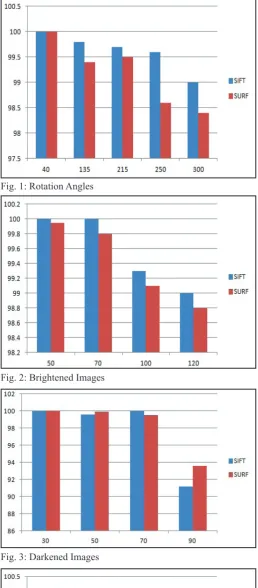
III. Experimental Results
For the purpose of obtaining our own experimental results, we have used a 64-bit Windows machine, with a Core i3 processor, running at 2.4 Ghz. For processing, MATLAB has been used. The results presented below are plots of matching accuracies against various parameters for both the SIFT and SURF detectors.
Fig. 1: Rotation Angles
Fig. 2: Brightened Images
Fig. 3: Darkened Images
Fig. 5: Blurred Images
As can be seen, the SIFT detector is a better choice with regard to distinctiveness.
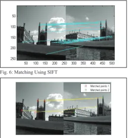
The results obtained when images are matched are as shown below.
Fig. 6: Matching Using SIFT
Fig. 6: Matching Using SURF
As can be seen from above, the SIFT detector-cum-descriptor performs very well with regards to matching different objects in the image. A few false matches were observed during the experimenting with the distance ratio values. The above results were obtained for a distance ratio of 0.45.
The computation times by the SIFT and SURF methods for the above process were respectively 2.61 and 0.82 seconds. The total number of keypoints found by the SIFT and SURF methods in both images are:
Table 1: Number of Keypoints
SIFT SURF
Image 1 252 98
Image 2 371 98
These were then applied to a non-standard image database of 7027 images, consisting of animals, butterflies, scenes, trees etc. and the results were satisfactory, with average times of computation being about 2.3 and 0.76 seconds respectively by SIFT and SURF methods.
IV. Conclusion
As seen, the SURF method is better when computation time is concerned, with sufficient accuracy. However, on considering the absolute accuracies, the SIFT method is much better owing to the large number of keypoints computed.
A number of other methods have also been devised, which have comparable performances to each of the two methods articulated here and it would be worthwhile to compare their performances in a different piece altogether.
References
[1] Lindeberg, T.,“Feature detection with automatic scale selection”, IJCV, Vol. 30, No. 2, pp. 79-116, 1998.
[2] Lowe, D.,“Distinctive image features from scale-invariant keypoints”, IJCV, Vol. 60, No. 2, pp. 91-110, 2004. [3] Mikolajczyk, K., Schmid, C.,“An affine invariant interest
point detector”, ECCV, pp. 128-142, 2002.
[4] Jasiobedzki, P., Moyung, T. J., Ng, H. K., Se, S.,“Vision based modeling and localization for planetary exploration rovers”, in Proceedings of International Astronautical Congress, 2004.
[5] Bay, H., Gool, L.V., Tuytelaars, T.,“SURF: Speeded up robust features”, In ECCV, 2006.
[6] Bischof, H., Grabner, H., Grabner, M.,“Fast approximated SIFT”, ACCV, Vol. 1, pp. 918-927, 2006.
[7] Harris, C., Stephens, H.,“A Combined Corner and Edge Detector”, In Alvey Vision Conference, 1988.
[8] Bauckhage , C., Schmid, C., Mohr, R.,“Evaluation of interest point detectors”, International Journal of Computer Vision, Vol. 37(2), pp. 151–172, 2000.
[9] Canny, J F,“Finding Edges and Lines in Images”, MIT technical report AI-TR-720, 1983.
[10] Moravec, H,“Obstacle Avoidance and Navigation in the Real World by a Seeing Robot Rover”, Tech Report CMU-RI-TR-3, Carnegie-Mellon University, Robotics Institute, September 1980.
[11] Schmid, C., Mohr, R.,“Local grayvalue invariants for image retrieval”, IEEE Trans. on Pattern Analysis and Machine Intelligence, 19(5), pp. 530–534, 1997.
[12] Koenderink, J.J.,“The structure of images”, Biological Cybernetics, 50, pp. 363–396, 1984.
[13] Lindeberg, T.,“Scale-space theory: A basic tool for analysing structures at different scales”, Journal of Applied Statistics, 21(2), pp. 224–270, 1994.
[14] Mikolajczyk, K.,“Detection of local features invariant to affine transformations”, Ph.D. thesis, Institut National Polytechnique de Grenoble, France, 2002.
[15] Brown, M., Lowe, D.G.,“Invariant features from interest point groups”, In British Machine Vision Conference, Cardiff, Wales, pp. 656–665, 2002.
Joy Gopal Goswami received his B.E. degree from Jorhat Engineering College in 2013 and is presently pursuing M.E. in Electrical Engineering from Jorhat Engineering College. His research interest includes image processing and he is presently working upon his academic dissertation on “Content-based image retrieval”.