Traffic Density Analysis based on Image
Segmentation with Adaptive Threshold
Luong Anh Tuan Nguyen
Ho Chi Minh City University of Transport No. 2, D3 Street, Ward 25, Binh Thanh District
Ho Chi Minh City, Vietnam
Thi-Ngoc-Thanh Nguyen
Ho Chi Minh City University of Transport No. 2, D3 Street, Ward 25, Binh Thanh District
Ho Chi Minh City, Vietnam
ABSTRACT
Traffic congestion has become an important problem in recent years. The main reason is the increase in the population in big cities and respective increase in number of vehicles. Traffic jams not only affect the human routine lives but also lead to a rise in the cost of transportation. So, an automatic traffic control system is required to manage the traffic congestion problem. The traffic den-sity analysis will support the traffic management problems such as intelligent traffic signal control, traffic planning, etc. This pa-per has proposed a traffic density analysis method based on im-age segmentation with adaptive threshold. The system was de-signed and evaluated with the traffic images taken in Ho Chi Minh City, Viet Nam. The proposed method provides a accuracy anal-ysis rate higher than 97% and a verification error lower than 3%.
General Terms
Traffic Density, Otsu threshold, Image Segmentation, Histogram
Keywords
Traffic Density, Otsu threshold, Image Segmentation, Histogram
1. INTRODUCTION
The calculation of traffic density is utilized for traffic control with different purposes. The density calculation helped in au-tomatic traffic lights switching for better traffic management. A lot of researches and works have been done on traffic analysis using image processing techniques. The authors of [1] discussed a model to count the traffic load by some parameters such as edge detection, histogram equalization, labeling and removing the noise with the help of median filter. The authors of [2] has proposed an approach to road monitoring and traffic problem, such as vehicle tracking, speed measurement, jam detection and number-plate recognition. The authors of [3] has proposed au-tomated vehicle detection based on average filter to reduce the noise effect. Thresholding value is applied to remove the un-wanted objects other than the vehicle. The authors of [4] sug-gested algorithm to determine the number of vehicles on the road and to control the traffic by calculating density only on the target area. There are several other methods of identifying traffic den-sity [5, 6], although these techniques are effective but the calcu-lation is so complicated.
It found that a traffic image with very crowded traffic density, the traffic vehicles will appear most of image and a traffic image with sparse traffic density, the background will appear most of image. This paper based on image segmentation method to clas-sify a traffic image into two classes including background and traffic vehicles with adaptive threshold. Each traffic image has a private adaptive threshold. The calculation of adaptive threshold was improved from Otsu threshold and histogram of grayscale traffic image. This paper was improved from our previous works [7, 8].
The rest of the paper is organized as follows. The theoretical background is discussed in Section 2. Section 3 presents the de-sign of system architecture. In section 4, the numerical results of experiment are illustrated. Finally, Section 5 concludes this paper and figures out the future works.
2. THE THEORETICAL BACKGROUND
2.1 Color Image
Color image [9, 10] is presented by a triple RGB (Red, Green, Blue). The value of color channels ranges from 0 to 255. Set of 3 color channels will generate224colors (256 * 256 * 256 colors).
2.2 Grayscale Image
Grayscale images [9, 10, 13] are the color images using RGB color system in which the Red, Green, Blue have the same light intensity. So, the grayscale image just need to use one light inten-sity to show each pixel. The gray level of grayscale image ranges from 0 to 255. There are some techniques to convert color image into grayscale image such as lightness with the equation (max(R, G, B) + min(R, G, B))/2, luminosity with the equation 0.21R + 0.72G + 0.07B.
2.3 Binary Image
A binary image [9, 10, 14] is a digital image that has only two possible values for each pixel. Typically, the two colors used for a binary image are black and white. The color used for the ob-ject(s) in the image is the foreground color while the rest of the image is the background color.
2.4 Histogram
Histogram [11, 12, 13] is the chart that shows the frequency of occurrence of each gray level in an image. Calculating histogram of image is performed as follows:
(1) Building the pixel matrix of the grayscale image.
(2) From the pixel matrix of the grayscale image, building the frequency of pixel.
3. SYSTEM ARCHITECTURE
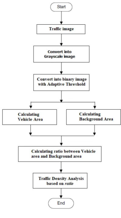
System architecture is depicted in Figure 1 and performed as fol-lows:
(1) Get traffic image from disk or other resources. (2) Converting traffic image into grayscale image.
(3) Converting grayscale image into binary image with adaptive threshold .
(4) Calculating vehicle area based on binary image. (5) Calculating background area based on binary image. (6) Calculating ratio between vehicle area and background area. (7) Traffic Density Analysis based on ratio between vehicle area
Fig. 1. The process of the training phase.
3.1 Converting Traffic Image into Grayscale Image
In this paper, the average method is selected, so the value of pixel in grayscale image is defined as (1).
V = (R+G+B)/3 (1)
3.2 Converting Grayscale Image into Binary Image with Adaptive Threshold
The pixel value of grayscale image ranges from 0 to 255. The equation (2) is used to convert grayscale image into binary image with threshold T.
g(x, y) =
0, f(x, y)< T
1, f(x, y)>=T (2)
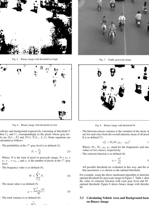
Using the fixed threshold is simple, but the result will be not ef-fective. Figure 2, Figure 3 and 4 show color image, grayscale image and binary image with fixed threshold, respectively. Fig-ure 5 and 6 show binary image with the value of threshold too high and too low.
It found that the traffic binary images will only include back-ground and traffic vehicles. However, the traffic binary image has some details not fully displayed. Therefore, the problem is to find a method to get the optimal threshold aim to limit this problem.
In this paper, the adaptive threshold based on the histogram of grayscale image to determine. The adaptive threshold based on otsu threshold [15, 16, 17] to determine as follows:
Gray levels of grayscale image range from 0 to L-1. Suppose that the image is separated into two categoriesC0 andC1 as
Fig. 2. Traffic color image
Fig. 3. Traffic grayscale image
Fig. 5. Binary image with threshold too high
Fig. 6. Binary image with threshold too low
vehicles and background respectively consisting of threshold T, thenC0 andC1correspondingly to the pixels whose gray
lev-els are{0,1,...,T}and{T+1, T+2,..., L-1}. Some equations are calculated as follows:
- The probability at theithgray level is as defined (3).
Pi= ni
N (3)
Where, N is the total of pixel in grayscale image, N =n0 +
n1+ ... +nL−1andniis the number of pixels at theithgray level.
- The frequency value is as defined (4).
W=
T
X
i=0
Pi (4)
- The mean value is as defined (5).
µ=
PT i=0iPi
W (5)
- The total variance is as defined (6).
σ2t = T
X
i=0
(i−µ)2Pi (6)
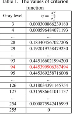
Fig. 7. Traffic grayscale image
Fig. 8. Binary image with threshold 94
- The between-classes variance is the variation of the mean val-ues for each class from the overall intensity mean of all pixels. It is as defined (7).
σ2b=W0W1(µ1−µ0)2 (7)
Where,W0,W1,µ0,µ1 stand for the frequencies and mean
values of two classes, respectively. - The criterion function is as defined (8).
η=σ
2
t σ2
b
(8)
All possible threshold are evaluated in this way, and the one that maximizesηis chosen as the optimal threshold.
For example, using the above mentioned algorithm to determine optimal threshold for grayscale image in Figure 7. Table 1 shows the value of criterion function with each gray level and 94 is optimal threshold. Figure 8 shows binary image with threshold 94.
3.3 Calculating Vehicle Area and Background based on Binary Image
white. Vehicles area is calculated by counting the pixels with the non-zero value and background area is calculated by counting the pixels with the zero value.
3.4 Traffic Density Analysis based on The Ratio between Vehicle Area and Background Area
The ration between vehicle area and background area is is de-fined as (9).
Ratio= V ehicles Area
Backgorund Area (9)
3.5 Traffic Density Analysis
Traffic density based on the ratio between vehicle area and back-ground area as follows:
- The ratio ranges from 0 to 0.25: Sparse Traffic Density - The ratio ranges from 0.25 to 0.5: Normal Traffic Density - The ratio ranges from 0.5 to 0.75: Crowded Traffic Density - The ratio ranges from 0.75 to 1: Very Crowded Traffic Density
4. EXPERIMENTAL RESULTS
4.1 Dataset
In this paper, 300 traffic images were taken in Ho Chi Minh city, Viet Nam on many different streets with different times. These images with the traffic density such as very crowded traf-fic, crowded traftraf-fic, normal traffic and sparse traffic are exper-imented in proposed technique. 300 images are divided into 3 subsets, each subset contains 100 traffic images.
4.2 Experiment Procedure and Results
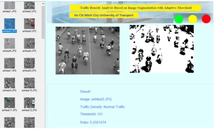
A system is designed by VB.NET programming language to ex-periment the proposed method with three subsets. The proposed method uses root mean square error (RMSE) [18] to measure accuracy. The correct analysis rates in percent are included in Table 2. Each result is the average of 100 runs, where we have randomly shuffled the traffic image in each run. Figure 9, 10 and 11 show the detail results of 100 runs. Figure 13 , 14 , 15 and 16 show some experimental results with four traffic densities.
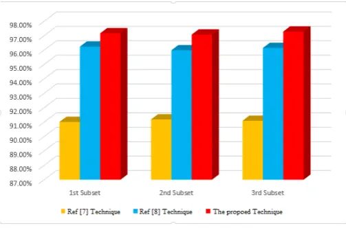
4.3 Comparing to other works
The performance of Ref [7] and Ref [8] based systems in the same setup is lower than the proposed method. Table 3 shows
Table 1. The values of criterion function
Gray level η=σ 2 t σ2 b 3 0.000300866239180 4 0.000596484071193 ... ... 28 0.183404567027206 29 0.192019758479230 ... ... 93 0.445166021994200 94 0.445399906387494 95 0.445369258716008 ... ... 126 0.318034391145754 127 0.315986641011137 ... ... 254 0.000875942416999 255 0
Table 2. The experimental results
Subset Analysis rates Time for analyzing an image (ms)
1st 97.16% 14
2nd 97.07% 11
3rd 97.28% 12
Fig. 9. The detail results of 100 runs - the first subset
Fig. 10. The detail results of 100 runs - the second subset
the results of the comparison between the proposed method and the work Ref [7] and Ref [8] with the same three subsets. The results of the comparison are depicted in Figure 12.
Table 3. The results of the comparison to other works.
Subset Ref [7] Technique Ref [8] Technique The proposed method
1st 91.02% 96.23% 97.16%
2nd 91.18% 95.98% 97.07%
3rd 91.09% 96.14% 97.28%
5. ACKNOWLEDGMENTS
The authors wish to thank reviewers for their reading of our manuscript and their insightful comments and suggestions.
6. CONCLUSIONS
In this paper, the traffic density analysis technique based on image segmentation with adaptive threshold has proposed. The technique is designed and experimented via Visual Studio with 300 images taken in Ho Chi Minh city, Viet Nam on many dif-ferent streets with difdif-ferent times. The best result was obtained with 97% accuracy.
Fig. 11. The detail results of 100 runs - the third subset
Fig. 12. The results of the comparison
7. REFERENCES
[1] Pratishtha Gupta , Purohit , Adhyana Gupta,Traffic Load Computation using Matlab Simulink Model Blockset In-ternational Journal of Advanced Research in Computer and Communication EngineeringVol. 2, Issue 6, June 2013 [2] Atkociunas, Blake, Juozapavicius Kazimianec Image
pro-cessing in road traffic analysis Nonlinear Analysis: Model-ing andControl, 2005, Vol. 10, No. 4, 315332
[3] Bharti Sharma, Vinoth Kumar Katiyar, Aravind Kumar Gupta, and Akansha Singh.(2014) The Automated Ve-hicle Detection of Highway Traffic images by Differ-ential Morphological Profile. Journal of Transportation Technologies,4,150-156.
[4] Dharani.S.J, Anitha.V, Traffic Density Count by Optical Flow Algorithm using Image Processing,Automative Parts system and Application, ISSN 2347-6710(paper) Volume 3,Special Issue 2. April 2014.
[5] Ozkurt C, Camci F. Automatic traffic density estimation and vehicle classification for traffic surveillance systems using Neural Networks. Mathematical and Computational Applications. 2009; 14(3):18796.
[6] C. Stuiz, T. A. Runkler, Classification and Predicts of Road Traffic using Application Specific Fuzzy Clustering, Fuzzy Systems, IEEE Transactions, pp. 297-308, 2002.
[7] Luong Anh Tuan Nguyen and Thi-Ngoc-Thanh Nguyen. Traffic Image Classification using Horizontal Slice Al-gorithm. International Journal of Computer Applications 148(11):30-34, August 2016.
[8] Luong Anh Tuan Nguyen and Thi-Ngoc-Thanh Nguyen. Traffic Density Identification based on Neural Network and Histogram. International Journal of Computer Applications 172(9):8-13, August 2017.
[9] Al Bovik, Handbook of Image and Video Processing, Aca-demic Press, 2000.
[10] Gonzalez, R., C., and Woods, R., E., 2001, Digital Image Processing, Prentice Hall, NJ, 2001
[11] Luong Anh Tuan Nguyen, Huu Khuong Nguyen. Traf-fic Density IdentiTraf-fication Based On Histogram. Journal of Transportation Science and Technology, ISSN: 1859-4263, Vol 15-05/2015, pp 23-27.
[12] C. C. Sun. S. J. Ruan, M. C. Shie, T. W. Pai, Dynamic Con-trast Enhancement based on Histogram Specification, IEEE Transactions on Consumer Electronics, 51(4), pp.1300-1305, 2005.
[13] Xiangyun Ye, Mohamed Cheriet, Senior Member, Ching Y. Suen (2001), Stroke-Model-Based Character Extraction from Gray-Level Document Images, IEEE, 2001.
[14] Binary Image (June, 2018), https :
//en.wikipedia.org/wiki/Binaryimage
[15] Otsu, N., ”A Threshold Selection Method from Gray-Level Histograms,” IEEE Transactions on Systems, Man, and Cy-bernetics , Vol. 9, No. 1, 1979, pp. 62-66.
[16] T. Bouwmans. Traditional and recent approaches in back-ground modeling for foreback-ground detection: An overview. Computer Science Review , 1112:31 66, 2014.
[17] Nida M. Zaitouna, Musbah J. Aqel. (2015). Survey on Im-age Segmentation Techniques. International Conference on Communication, Management and Information Technol-ogy (ICCMIT). pp 797 806.
Fig. 13. The result of Sparse Traffic density
Fig. 15. The result of Crowded Traffic density