University of Khartoum
Faculty of engineering and architecture
Department of electrical and electronic engineering
Study of Fast packet switches architectures
for Asynchronous Transfer mode
By: Nassir Mohammed Elbakri Elzein
Supervised by: D. ElRasheed Osman Khidir
A thesis submitted for partial fulfillment of the degree of
M.Sc in telecommunication and information systems
Dedication
For Mohanned’s soul who was more than a friend…. For my family…
For Sudan… For Science….
Acknowledgement
I would like to thank my supervisor, Dr. Elrasheed Osman Khidir, for his generous assistance and support.
Special thanks go to every one who contributed with an idea or experience to this work, specially my friend Haytham Mohammed Osman who has helped in the computer simulation implementation, who was very helpful
Surely my appreciation goes to my parents and my wife and sisters without whose support I would never made it to this point.
ﺺﻠﺨﺘﺴﳌﺍ
ﻟﺍ ﺎﻜﺒﺸ ﺕ ﺔﻠﻣﺎﻜﺘﳌﺍ ﺕﺎﻣﺪﺨﻠﻟ ﺔﻴﻤﻗﺮﻟﺍ ﻟﺍ ﺔﻀﻳﺮﻋ ﻕﺎﻄﻨ ﺮـﺜﻛﻷﺍ ﻞـﳊﺍ ﻮﻫ ﻦﻣﺍﺰﺘﳌﺍ ﲑﻏ ﻞﻘﻨﻟﺍ ﺏﻮﻠﺳﺃ ﺎﻬﻴﻓ ﱪﺘﻌﻳ ،ﹰﻻﻮﺒﻗ ﺕﺎﻜﺒﺸﻟﺍ ﻩﺬﻫ ﱃﺇ ﺝﺎﺘﲢ ﻡﺰﺣ ﻞﻳﻮﲢ ﺏﻮﻠﺳﺃ ﻊﻳﺮﺳ ﻲـﺿﺍﺮﺘﻓﻻﺍ ﺭﺎﺴﳌﺍ ﱪﻋ ﻦﻣﺍﺰﺘﳌﺍ ﲑﻏ ﻞﻘﻨﻟﺍ ﺏﻮﻠﺳﺃ ﺎﻳﻼﺧ ﻞﻘﻨﻟ ﺎﳍ ﺺﺼﺨﳌﺍ . ﺔﻴﺳﺎﺳﻷﺍ ﺔﻔﻴﻇﻮﻟﺍ ﻢﺴﻘﳌ ﳌﺍ ﲑﻏ ﻞﻘﻨﻟﺍ ﺏﻮﻠﺳﺃ ﺝﺮـﺨﳌﺍ ﱄﺍ ، ﺩﺪﳏ ﻞﺧﺪﻣ ﱄﺍ ﻞﺼﺗ ﱵﻟﺍ ﺎﻳﻼﳋﺍ ﻪﻴﺟﻮﺗ ﻮﻫ ﻦﻣﺍﺰﺘ ﺝﻭﺮﳋﺍ ﺀﺎﻨﻴﲟ ﹰﺎﻀﻳﺃ ﻑﺮﻌﻳ ﻱﺬﻟﺍﻭ ﺎﳍ ﺺﺼﺨﳌﺍ . ﻩﺬﻫ ﻦﻣ ﻑﺪﳍﺍ ﺔﺳﺍﺭﺪﻟﺍ ، ﺔﻴﺴﻴﺋﺮﻟﺍ ﺙﻼﺜﻟﺍ ﻕﺮﻄﻟﺍ ﺔﺸﻗﺎﻨﻣ ﻮﻫ ﻣﺪﺨﺘﺴﳌﺍ ﺔ ﺀﺎﻨﺒﻟ ﻢﺳﺎﻘﳌﺍ ﻲﻫﻭ : ﺕﺎﺣﺎﺴﳌﺍ ﻢﻴﺴﻘﺗ ﺔﻛﺮﺘﺸﳌﺍ ﺓﺮﻛﺍﺬﻟﺍﻭ ، ﺔﻛﺮﺸﳌﺍ ﻂﺋﺎﺳﻮﻟﺍ ، . ﻷﺍ ﺔﻠﺜﻣﻷﺍ ﻦﻣ ﳌ ﺔﻴﺳﺎﺳ ﻢﺴﻘ ﺕﺎﺣﺎﺴﳌﺍ ﻢﻴﺴﻘﺗ ﻢﺴﻘﻣ ﻮﻫ ﰲ ﹰﺎﻘﺑﺎـﺳ ﻡﺪﺨﺘﺴـﻳ ﻥﺎﻛ ﻱﺬﻟﺍﻭ ﺽﺮﻌﺘﺴﳌﺍ ﺐﻴﻀﻘﻟﺍ ﺮﺋﺍﻭﺪﻟﺍ ﻞﻳﻮﲢ ﻡﺎﻈﻨﺑ ﻞﻤﻌﺗ ﱵﻟﺍ ﻒﺗﺎﳍﺍ ﺕﺎﻜﺒﺷ . ﻲﻤﺴـﺗ ﻞﻳﻮﲢ ﻁﺎﻘﻧ ﰲ ﺎﻬﻄﺑﺭ ﻢﺘﻳ ﻝﻮﶈﺍ ﺍﺬﻫ ﰲ ﺝﺮﳋﺍﻭ ﻞﺧﺪﻟﺍ ﺬﻓﺎﻨﻣ ﺕﺎﻓﻮﻔﺼﻣ ﻞﻜﺷ ﻲﻠﻋ ﺔﻴﻨﺑ ﺔﺠﻴﺘﻨﻟﺍ ﻥﻮﻜﺗﻭ ﺔﺿﺮﻌﺘﺴﳌﺍ ﻁﺎﻘﻨﻟﺍ . ﻮﻧ ﺮﻳﻮﻄﺗ ﰎ ﹰﺍﺮﺧﺆﻣ ﺐﻴﻀـﻘﻟﺍ ﺕﻻﻮـﳏ ﻦـﻣ ﺪﻳﺪﺟ ﻉ ﻩﺬﻫ ﰲ ﻉﻮﻨﻟﺍ ﺍﺬﻫ ﺔﺸﻗﺎﻨﻣ ﻢﺘﻴﺳﻭ ﺔﺟﺭﺎﳋﺍﻭ ﺔﻠﺧﺍﺪﻟﺍ ﺎﻳﻼﳋﺍ ﰲ ﻡﺎﺣﺰﻟﺍ ﻞﻴﻠﻘﺘﻟ ﺽﺮﻌﺘﺴﳌﺍ ﺔﺳﺍﺭﺪﻟﺍ . ﺪﻤﺘﻌﻳ ﻱﺮﺧﺃ ﺔﻴﺣﺎﻧ ﻦﻣ ﺔﻴﻟﺎﻋ ﺔﻋﺮﺳ ﻭﺫ ﻡﺎﻋ ﻞﻗﺎﻧ ﻲﻠﻋ ﺔﻛﺮﺘﺸﳌﺍ ﻂﺋﺎﺳﻮﻟﺍ ﻝﻮﳏ ﻞﻤﻋ . ﺭ ﺔﻘﻳﺮﻄﺑ ﻞﻗﺎﻨﻟﺍ ﱄﺍ ﻞﺧﺪﳌﺍ ﻦﻣ ﺎﻳﻼﳋﺍ ﻊﻓﺩ ﻢﺘﻳ ﺍ ﺪﻧﻭ ﻦﺑﻭﺭ ﻘﺘﺴﻳ ﺝﺮﳐ ﻞﻛﻭ ﻂﻘﻓ ﻪﻟ ﻪﺟﻮﳌﺍ ﺎﻳﻼﳋﺍ ﻞﺒ . ﻩﺬﻫ ﰲ ﺳﺍﺭﺪﻟﺍ ﻉﻮﻨﻟﺍ ﺍﺬﳍ ﺔﻴﻟﺎﻌﻓ ﺮﺜﻛﺃ ﺔﻴﻨﺑ ﺔﺸﻗﺎﻨﻣ ﻢﺘﻳ ﺔ ﻮﻫ ﻭ ﻡﺰـﳊﺍ ﻝﻮـﳏ ﻟﺍ ﻡﺎﻈﻧ ﻲﻠﻋ ﲏﺒﳌﺍ ﺕﺍﺭﺎﺴﳌﺍ ﺩﺪﻌﺘﻣ ﻦﻣﺰﻟﺍ ﻢﻴﺴﻘﺘﺑ ﺞﻣﺪ . ﻢﺴﻘﻣ ﺓﺮﻛﺍﺫ ﻲﻠﻋ ﻱﻮﺘﳛ ﺔﻛﺮﺘﺸﳌﺍ ﺓﺮﻛﺍﺬﻟﺍ ﺓﺪﻴﺣﻭ ﻣ ﺰ ﺔﺟﻭﺩ ﺊﻓﺍﺮﳌﺍ ﻞﺧﺪـﻟﺍ ﻁﻮﻄﺧ ﻊﻴﲨ ﲔﺑ ﺎﻬﺘﻛﺭﺎﺸﻣ ﻢﺘﻳ ﳋﺍﻭ ﺝﺮ . ﻟﺍ ﻡﺰﳊﺍ ﻁﻮﻄﺧ ﻊﻴﲨ ﱄﺍ ﻞﺼﺗ ﱵ ﻢﺘﻳ ﻞﺧﺪﻟﺍ ﺎﳍﺎﺧﺩﺇ ﻦﻳﺰـﺨﺘﻠﻟ ﺔﻣﺎﻋ ﺓﺮﻛﺍﺫ ﻱﺰﻐﻳ ﻱﺬﻟﺍﻭ ﺪﻴﺣﻭ ﺭﺎﺴﻣ ﰲ . ﰲ ،ﺔﻤﻈﺘﻨﻣ ﺝﺮﺧ ﻑﻮﻔﺻ ﰲ ﻡﺰﳊﺍ ﻢﻴﻈﻨﺗ ﻢﺘﻳ ﺓﺮﻛﺍﺬﻟﺍ ﻩﺬﻫ ﻞﺧﺍﺩ ﻞﻛ ﺝﺮﺧ ﺓﺪﺣ ﻰﻠﻋ . ﺭﺎﺴـﻣ ﻞﻤﻋ ﻢﺘﻳ ﺖﻗﻮﻟﺍ ﺲﻔﻧ ﰲ ﻢﺘﻳ ﰒ ﻦﻣﻭ ﻒﺻ ﻞﻜﻟ ﺪﺣﺍﻭ ، ﹰﺎﻌﺑﺎﺘﺗ ﺝﺮﳋﺍ ﻑﻮﻔﺻ ﻦﻣ ﻡﺰﳊﺍ ﺓﺩﺎﻌﺘﺳﺎﺑ ﻡﺰﺤﻠﻟ ﺝﺮﺧ ﺝﺮﳋﺍ ﻁﻮﻄﺧ ﱪﻋ ﻡﺰﳊﺍ ﻝﺎﺳﺭﺇ . ﻕﺮﻃ ﻦﻋ ﺢﺴﻣ ﻉﻭﺮﺸﳌﺍ ﻩﺬﻫ ﻡﺪﻘﻳ ﻢﻴﺴﻘﺗ ﺔﻄﻴﺳﻮﻟﺍ ﺓﺮﻛﺍﺬﻟﺍ ﻢﺳﺎﻘﳌ ﺎﻬﳝﺪﻘﺗ ﰎ ﱵﻟﺍ ﺍ ﻡﺰﺣ ﻟ ﻊـﺿﻭ ﰎﻭ ﺔﻛﺮﺘﺸـﳌﺍ ﺓﺮﻛﺍﺬ ﻟﺍ ﻦﻣ ﺪﻳﺪﻌﻟﺍ ﻕﺮﻄ ﻢﻴﺴﻘﺘﻟ ﻕﺮﻄﻟﺍ ﻩﺬﻫ ﻒﻌﺿﻭ ﺓﻮﻗ ﺭﺎﺒﺘﺧﺍ ﰎﻭ ﺔﻄﻴﺳﻮﻟﺍ ﺓﺮﻛﺍﺬﻟﺍ . ﻦﻣ ﺪﻳﺪﻌﻟﺍ ﺭﺎﺒﺘﺧﺍ ﰎ ﻕﺮﻄﻟﺍ ﻡﺍﺪﺨﺘـﺳﺎﺑ ﺳﺎﳊﺍ ﺔﻄﺳﺍﻮﺑ ﺓﺎﻛﺎﶈﺍ ﺏﻮ . ﰲ ﺓﺩﺭﺍﻮـﻟﺍ ﺞﺋﺎـﺘﻨﻟﺍﻭ ﺓﺎﻛﺎﶈﺍ ﺞﺋﺎﺘﻧ ﺓﺪﻋﺎﺴﲟ ﻕﺮﻄﻟﺍ ﻢﻫﻷ ﺔﻧﺭﺎﻘﻣ ﺹﻼﺨﺘﺳﺍ ﰎ ﺏﺭﺎـﺠﺘﻟﺍ ﺔﻘﺑﺎﺴﻟﺍ . ﺘﺴﳌﺍ ﺙﻮﺤﺒﻟﺍ ﺔﺸﻗﺎﻨﲟ ﺚﺤﺒﻟﺍ ﻢﺘﺧ ﰎ ﻢﺴﻘﻣ ﺔﻴﻨﺒﺑ ﺔﻄﺒﺗﺮﳌﺍﻭ ﺔﻨﻜﻤﳌﺍ ﺔﻴﻠﺒﻘ ﻊﻳﺮﺴﻟﺍ ﻡﺰﳊﺍ .Abstract
Broadband ISDN networks, of which ATM is the accepted transfer mode solution, require fast packet switches to move the ATM cells along their respective virtual paths. The prime purpose of an ATM switch is to route incoming cells (packets more generally) arriving on a particular input link to the output link, which is also called the output port, associated with the appropriate route. The subject of this thesis is to discuss the three basic techniques that have been proposed to carry out the switching (routing) function: space-division, shared-medium, and shared-memory. The basic
example for a space-division switch is a crossbar switch, which has also served circuit-switched telephony networks for many years. The inputs and outputs in a crossbar switch are connected at switching points called crosspoints, resulting in a matrix type of structure. New decomposed crossbar switches architecture is developed recently so as to minimize the input and output cell contention, this new architecture is discussed in this thesis. The operation of a shared-medium switch, on the other hand, is based on a common high-speed bus. Cells are launched from input links onto the bus in round-robin fashion, and each output link accepts cells that are destined to it. A more enhanced architecture of this type; a TDM-Based Multibus Packet Switch is discussed in this project. The shared-memory
(SM) switch, consists of a single dual-ported memory shared by all input and
output lines. Packets arriving on all input lines are multiplexed into a single stream that is fed to the common memory for storage; inside the memory, packets are organized into separate output queues, one for each output line. Simultaneously, an output stream of packets is formed by retrieving packets from the output queues sequentially, one per queue; the output stream is then demultiplexed, and packets are transmitted on the output lines. This project presents a survey of the buffer management methods that have been proposed for shared-memory packet switches. Several buffer management policies are described, and their strengths and weaknesses are examined. The performances of various policies are evaluated using computer simulations. A comparison of the most important schemes is obtained with the help of the simulation results and the results provided in the literature. The survey concludes with a discussion of the possible future research areas related to the Fast packet switch architectures.
List of Abbreviation
AF Address Filter
ATM Asynchronous Transfer Mode
ATOM ATM Output Buffer Modular Switch CAC Connection Admission Control CBR Constant Bit Rate
CIOQ Combined Input Output Queue CLR Cell Loss Ratio
CMOS Complementary Metal Oxide Semiconductor CP Complete Partitioning
CS Complete Sharing
CSVP Complete Sharing with Virtual Partition DE Distribution Element
DoD Drop on Demand
DRAM Dynamic Random Access Memory DRP Delay Resolution Policy
DT Dynamic Threshold
FIFO First In First Out
HB Horizontal Bus
HOL Head Of Line
I/O Input/Output
IC Integrated Circuits
IP Internet Protocol
ISDN Integrated Service Digital Network LAN Local Area Network MAC Media Access Control
OQ Output Queue
PARIS Packetized Automated Routing Integrated System P/S Parallel / Serial
PCM Pulse Code Modulation
PIPN Plane interconnected Parallel Network
PO Push Out
POT Push Out with Threshold PPS Parallel Packet Switches QoS Quality of Service
Rn Randomly loaded Parallel Networks RTT Round Trip Time
S/P Serial/Parallel
SE Switching Element
SF Speed up Factor
SM Shared Memory
SMA Sharing with minimum Allocation
SMQMA Sharing with Maximum Queue and Minimum Allocation SMXQ Sharing with Maximum Queue length
Sn Selectively Loading Parallel Network SRAM Static Random Access Memory
ST Static Threshold
TCP Transport Control Protocol TDM Time Division Multiplexing
VB Vertical Bus
VLSI Very Large Scale Integrated Circuit WAN Wide Area Network
Index
Dedication………...I Acknowledgement………..II ﺔﺻﻼﺨﻟا ………III Abstract………...IV List of Abbreviations……….….V Chapter 1 Introduction1.1 Statement of the problem……….………….1
1.2 Background review..……….………1
1.2.1 Fast packet switching definition……….……….1
1.2.2 Networking and switching……….………..2
1.2.3 Store and forward and channel utilization………….………..4
1.2.4 Integrated service Digital Network……….……….6
1.2.5 Broad band ISDN and Fast Packet switching……….….7
1.2.6 Packet switch definition and functionality……….…..7
1.2.7 Traffic pattern and packet switch performance….…………...9
1.3 Objectives………..9
1.4 The approach………....11
1.5 The body of the research………..11
1.6 Layout of the project………11
Chapter 2 Space division fast packet Switch 2.1 Crossbar Architecture……….….13
2.2 Banyan network………...13
2.3 Replication technique of Banyan networks……….…15
2.4 Plane Interconnected Parallel Network(PIPN)………....15
2.4.1. The replicated PIPN switch structure………....18
2.5 Comment ...………..19
Chapter 3 Shared Medium fast packet switch 3.1 Introduction………..…....20
3.2 The TDM-based multi bus packet switch....……….21
3.2.1 Architecture………...21
3.3 Comment……….26
Chapter 4 Shared Memory fast packet switch 4.1 Introduction……….27
4.2 Types of Memory………29
4.2.1 SRAM only....……….29
4.2.2 SRAM and DRAM……….30
4.2.2.1 Statistical Guarantees…...……….31
4.2.2.2 Deterministic Guarantees………..31
4.2.3 DRAM Only………...31
4.2.3.1 Techniques which rely on the DRAM row or bank properties………..32
4.2.3.2 Techniques which provide statistical guarantees………..32
Chapter 5 Output buffer management for ATM switch 5.1 Introduction……….33
5.2 Buffer Allocation Policies………...34
5.2.1 Static Thresholds...……….………35
5.2.1.1 Complete Partitioning and Complete sharing…………...35
5.2.1.2 Sharing with Maximum Queue Lengths………...37
5.2.1.3 SMA and SMQMA………...37
5.2.2 Push-Out……….38
5.2.3 Dynamic Policies………....40
5.2.3.1 Adaptive Control………...40
5.2.3.2 Dynamic Threshold………...41
Chapter 6 Computer simulation for buffer management policies 6.1 Simulation program assumptions……….…………42
6.2 Programming language……….…………43
6.3 Generating on and off periods for negative exponential distribution………43
6.4 Program features ………..43
6.5 Program operation……….………44
6.6 Program Flow Chart……….………….46
Chapter 7 Conclusion
7.1 Space division type summary……….……..52 7.2 Shared medium type summary……….……....52 7.3 Comparative Summary of different buffer policies in shared
memory type ………...……….…52 7.4 Comments on the computer simulation……….…...53 7.5 future researches……….……..………53 Appendices
Program code………..…55 References………...64
CHAPTER 1
INTRODUCTION
1.1. Statement of the problem:
The telecommunication networks are divided into to major types, voice networks, and data networks. The different nature of voice and data has pushed the designers to dedicate separate network for each, circuit switching network for voice and packet switching network for data. But now the trend is to design a single communication system which supports all the services in an integrated and unified fashion. The switching technique emerging to be the most appropriate is the packet switching. It’s clearly the appropriate technique to use for data applications with bursty traffic ; it also offer greater flexibility than circuit switching in handling the wide diversity of data rates and latency requirements resulting from the integration of services. One main challenge therefore has been to design and build packet switches capable of switching relatively small packets at extremely high rates (say 100 00 to 1000000 packets per second per line).
1.2. Background review
In order to go through various architectures of the fast packet switch; some concepts and definitions must be first introduced.
1.2.1. Fast Packet switching Definition:
Packet switching refers to protocols in which messages are divided into packets before they are sent. Each packet is then transmitted individually and can even follow different routes to its destination. Once all the packets forming a message arrive at the destination, they are recompiled into the original message.
Most modern Wide Area Network (WAN) protocols, including TCP/IP, X.25, and Frame Relay, are based on packet-switching technologies. In contrast, normal telephone service is based on a circuit-switching technology, in which a dedicated line is allocated for transmission between two parties. Circuit-switching is ideal when data must be transmitted quickly and must arrive in the same order in which it's sent. This is the case with most real-time data, such as live audio and video. Packet
switching is more efficient and robust for data that can withstand some delays in transmission, such as e-mail messages and web pages.
A new technology, ATM, attempts to combine the best of both worlds; the guaranteed delivery of circuit-switched networks and the robustness and efficiency of packet-switching networks.
1.2.2. Networking and switching
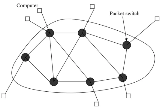
Networking refers to the configuration of transmission facilities into a network that can serve a number of geographical distributed users. Geographically distribution does not imply that users are widely separated, although the distance may affect the type of network required. As fully connected topology for a network serving N sites requires N (N-1)/2 links and this is practical only for small N.
Figure .1.1 shows a topology of partially connected nodes
Fig .1.1 partially connected topology.
Switching on the other hand refers to the means by which to allocate the limited transmission facilities to the users so as to provide a certain degree of connectivity among them. Thus the combination of networking and switching is what provide connectivity among users in an economic and efficient way.
Although we find today a variety of networks designed to meet different needs, they are all based on two principal switching techniques, called circuit switching and packet switching.
In circuit switching, a complete path of connected links from the origin to the destination is set up at the time the call is made, and the path remain connected and dedicated to that call until is released by the communicating parties. The path is set up by special signaling message that finds its way through the network from the origin to the destination. Once the path is completed, a return signal informs the source of that fact, and the source can then begin to transmit. From this point on, the switches are virtually transparent to the transfer of information from the source to the destination; that is for all practical purposes, the two end users have a continuous circuit connecting them for the entire duration of the conversation. Circuit switching is used in the telephone network for voice communication.
In data communications applications, the exchange of information among users takes place in the form of blocks of data referred to as messages. To best fit the characteristics and requirements of such exchanges, message switching has been introduced. For transmission purposes, a massage consists of a user’s data to be transmitted, a header containing control information (e.g., source and destination addresses, message type, priority, etc.) and a checksum used for error control purposes. The switches are computers with special processing and storage capabilities. Consider for example a wide area network with a general mesh topology (see fig1.2).
First the message is transmitted from the user device to the switch to witch it is attached. Once the message is entirely received, the switch examines its header, and selects the next transmission channel on which to forward the message accordingly; the same process is then used from switch to switch until the message is delivered to its destination. (This transmission technique is also appropriately referred to as the store-and-forward technique.)
Fig .1.2. A wide area computer communications network.
1.2.3. Store and forward and channel utilization
Circuit switching is likely to be cost effective only on those situations where, once the circuit is set up; there will be a relatively steady flow of information. This is certainly the case of the voice communication, so circuit switching is the technique commonly used in the telephone system. Communication among computers, however, tends to be bursty. Burstiness is characterized by random gaps encountered in the message- generation process, variability of the message size, and the low tolerance of delay by the user. The users and devices require the communication resources relatively infrequently; but when they do, a relatively rapid response is important. If an end to end circuit were to be set up connecting the end users, then one must assign sufficient transmission bandwidth to the circuit in order to meet the delay constraint; given the random gaps in the message generation process, the resulting channel utilization is low. If the circuit of
Computer
request, then the set up time incurred with each request would be large compared to the transmission time of the message, resulting again in low channel utilization. For bursty users, store – and-forward transmission technique offer a more efficient solution, as a message occupies a particular communications link only for the duration of it’s transmission on those links; the rest of the time it is stored at some intermediate switch and the links are available for transmission of other messages. The main characteristic of store-and-forward transmission over circuit switching is that the communication bandwidth is dynamically allocated, and the allocation is done on the basis of a particular link in the network and a particular message (for a particular source-destination pair).
Packet
switching is a variant of message switching. Here, the blocksof data that can be transmitted over the network are not allowed to exceed a given maximum length; they are referred to as packets. Messages exceeding that length are broken up into several packets which are transmitted independently in a store -and -forward manner. Packet switching achieves the benefits discussed so far of message switching and offer added features. It provides the full advantage of the dynamic and fair allocation of the bandwidth, even when the message varies considerably in length.
Here are some advantages of packet switching over message switching [1]:
• With packet switching, the end-to-end transmission delay of a message is smaller than that of achieved with message switching due to pipelining effect; that is many packets of a message may be in transmission simultaneously over successive links of a path from source to destination.
• Packet switching tends to require smaller storage capacities at all the intermediate switches, owing to their limited size,
• Packets are less likely to be rejected at a node than are full size messages.
• Error recovery procedure tends to be more efficient with packet switching because, again owing to their limited size. Packets are less prone to transmission errors than messages; and when an error does occur in a packet over a transmission line, only that packet needs to be retransmitted on that link.
arrive at the destination out of order. The efficient utilization of transmission facilities, coupled with the continuous progress in digital processing technology, has rendered packet switching the more economical and thus preferred mode of switching for data communication since its introduction in the late sixties.
1.2.4 Integrated service Digital Network
Today, the trend is toward the design of a single communications system which provides all services simultaneously in a unified fashion.
Originally, analogue transmission was used throughout the telephone network. With the advent of digital signal processing and computer technologies, digital switches and digital transmission facilities gradually replaced electromechanical switches and the analog facilities between them. Internal to the network speech signal is digitized using pulse-code modulation (PCM), producing data at the constant rate of 64Kb/s, and thus a voice channel becomes merely a 64Kb/s data channel, subscribers loops (the twisted pairs connecting the user telephone to the central office), however, remain analog. (That is why data transmission over the telephone network requires the use of a modem.) ISDN extends digital transmission capabilities to the existing twisted pair loop and provide the subscriber with two 64Kb/s circuit switched channels (called the B channels) and one 16Kb/s packet switched channel (called the D channel). The D channel carries the signaling information needed to manage the two B channels and may carry some user data in packet mode. Business subscribers can be provided with a primary rate equal to 2.048 Mb/s, the rate available on E1 carriers. Thus with ISDN,
digital communication at the aggregate rate of 144 Kb/s is made available for homes and offices as easy as telephone services today.
The major characteristic of ISDN is that it is a public end to end digital telecommunication network, and as such it provides the basic communication capability for a wide range of user applications. An ISDN socket supports wide variety of devices including the telephone, a personal computer, a graphic station, a television, and devices yet to be invented, and would provide data transmission and switching capabilities from end to end communication. It eliminates in many instances the need for a separate data network.
One last note about narrow-band ISDN. Although the user sees an integration of services, internally the two switching techniques will remain at first isolated and provided separately. Existing circuit switches continue to
provide the end to end 64 Kb/s circuits regardless of weather they are used for voice or data, and separate packet switches are added to offer the packet switched service available in the D channels. Thus aside from the D channel, which is mostly for control and signaling, all the narrow-band ISDN offers subscribers is 64Kb/s end-to-end circuit for data transmission.
1.2.5 Broad band ISDN and Fast Packet Switching
The constant desire to achieve larger transmission bandwidth than is possible with radio or wire media has led to the consideration of optical communications.
While fiber optics technology provides the necessary bandwidth for transmission purposes, the creation of a network that can provide high bandwidth services to the users remains a challenge. The bottleneck comes primarily from switching. As it is projected that such high speed networks will carry all applications (voice, data video and images) in an integrated fashion, the most appropriate switching technique is emerging to be packet switching.
Thus the main challenge remains to build packet switches which can handle rates on the order of 100000 to 1000000 packets per second per input line. The first switches being considered for this purpose are being implemented electronically, using very large scale integrated circuit technology.
1.2.6 Packet switch definition and functionality
A packet switch is a box with N inputs and N outputs which routes the packets arriving of its inputs to their requested outputs. For simplicity we begin with the assumption that all lines have the same transmission capacity, all packets are of the same size, and that the arrival times of packets at the various input lines are time- synchronized, and we consider the operation of the switch to be synchronous. We also assume that each packet is destined to a single output port. However, there is no correlation among arriving packets as far as their destination requests are concerned, and thus more than one packet arriving in the same slot may be destined to the same output port. We refer to such an event as output conflict. Due to output conflicts, buffering of packets within the switch must be provided. Thus a packet switch is a box, which provides two functions: routing (or, equivalently, switching) and
An ideal switch is one that can route all packets from their input lines to their requested output lines without loss and with the minimum transit delay possible, while preserving the order in which they have arrived to the switch. The switch should also have sufficient buffering capacity so as not to lose any packet due to lack of buffers. (Note that if packets arriving in each slot present no conflicts, then virtually no buffering would be required.)
Besides the basic switching operation that is performed by a switch, there are two other functions that may at times be required. The first is multicast operation. Depending on the application being serviced, it may be necessary for a packet originating at a source node in the network to be destined to more than one destination. This could be accomplished by creating multiple copies of the packet at the source node, each destined to one of the desired destinations, and routing the copies independently. Alternatively, ,multicast routing may be achieved by requiring the switches in the network to have the capability to replicate a packet at several of their output ports, according to information provided for that purpose, thus reaching the multiple destinations from a single packet originating at the source. This mode of operation results in lower traffic throughout the network but at the expense of higher complexity in switch design. The second function that may be required of a switch is the priority function. It consists of the ability to differentiate among packets according to priority information provided in them, and to give preferential treatment to higher priority packets. Multicast and priority functions are achieved in the various architectures by various means, which are not going to be covered in this thesis.
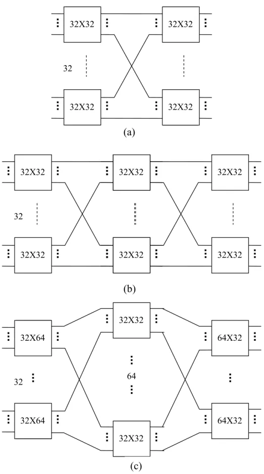
the technology used in implementing the switch places certain limitations on the size of the switch and line speeds; thus to build large switches, many modules are interconnected in a multistage configuration, which provides multiple paths from the inputs to the outputs, thus offering the concurrency required to handle the large size. See fig.1.5 (a) shows the configuration with only one path between an input and an output, (b) shows the configuration with 32 different paths between each input and output, and(c) shows the configuration with 64 different paths between each input and output.
1.2.7 Traffic pattern and packet switch performance
An important factor affecting the performance of a packet switch is the traffic pattern according to which packets arrive at its inputs. The traffic pattern is determined by:
1. The process which describes the arrival of packets at the inputs of the switch.
2. The destination request distribution for arriving packets.
The simplest traffic pattern of interest is one whereby the process describing the arrival of packets at an input line is a Bernoulli process with parameter p. independent from all other input lines, and whereby the requested output port for a packet is uniformly chosen among all output ports, independently for all arriving packets. Such a traffic pattern is referred to as the independent uniform traffic pattern. Other traffic pattern may actually arise which exhibit dependencies in the packet arrival processes as well as in the distribution of output ports requested. For example, packets may arrive at an input line in the form of bursts of random lengths, with all packets in a burst destined to the same output port. The traffic pattern in this case is defined in terms of the distributions of burst lengths, of the gap between consecutive bursts, and of the requested output port for each burst. Such a traffic pattern may be referred to as the bursty traffic pattern.
1.3 Objectives:
While the functionality required for a fast packet switch is quite simple and is practically the same as that required of packet switches used traditionally in computer networks, the challenge here is to design switches that meet the speeds required. Several architectural designs have emerged in the recent years. These may be classified into three categories; namely the space-division type, the shared-medium type and shared memory type.
Each of these categories presents features and attributes of its own which are identified in this survey.
Fig .1.5. The construction of large switches using modules in multistage configurations. 32X32 32X32 32X32 32X32 32 32X32 32X32 32X32 32X32 32 32X32 32X32 32X32 32X32 32X64 32X64 32X32 32X32 32 64X32 64X32 64 (c) (b) (a)
1.4 The approach:
The basic designs of fast packet switches for each type is first highlighted, then recent designs that proposed in literature are discussed. with the aid of computer simulation some designs are tested under various traffic conditions, the results of this experiments help in choosing the appropriate design for a given traffic nature.
1.5 The body of the research:
As mentioned before the basic three types of the packet switch architectures are the space division type, shared medium type and the shared memory type. In this thesis I concentrate in the shared memory type and I take the buffer management policy as the main subject of my computer simulation program
1.6 Layout of project:
The various architectures proposed for such fast packet switches are surveyed, and performance and implementation issues under-lying such architectures are discussed.
In this chapter an over view about fast packet switching and its different technologies are discussed, this over view gives some general ideas about the concepts and principals that packet switches are based on.
In the second chapter space division packet switch architecture is discussed and a recent architecture of this type is introduced using PIPN technique, this technique adds more enhancements to the space division type.
The third chapter is focusing on shared-medium fast packet switches and discussing the architecture of the TDM-based multi-bus packet switch.
The shared memory switches basic architectures and techniques of using different types of memory for this type are discussed in chapter 4.
Discussion of different policies of buffer management of a shared memory ATM switch is the topic of chapter 5.
In chapter 6 a computer simulation is introduced for evaluating the performances of some buffer management policies used in a shared memory ATM switch. The simulation results show the effect of the type of traffic on a certain policy.
In chapter 7 the thesis is concluded with a summary of the three types of the fast packet switches architectures and a comparative summary of different buffer policies in shared memory type, and the chapter ends with recommendation and future works.
CHAPTER 2
SPACE DIVISION FAST PACKET
SWITCH
2.1. Crossbar Architecture
Several architectural designs have emerged to implement the fast packet switch. As mentioned before they may be classified into three categories: the shared -memory type, the shared medium type, and the space -division type. Both shared - memory and shared -medium suffer from their strict capacity limitation, which is limited to the capacity of the internal communication medium. Any internal link is N times faster than the input link (where N is the number of inputs or outputs) and it is usually implemented as a parallel bus. This makes such architectures more difficult to implement as N becomes large.
The simplest space -division switch is the crossbar switch, which consists of a square array of NxN crosspoint switches, one for each input -output pair as shown in Fig.2.1. As long as there is no -output conflicts, all incoming cells can reach their destinations. If, on the other hand, there is more than one cell destined in the same time slot to the same output, then only one of these cells can be routed and the other cells may be dropped or buffered. The major drawback of the crossbar switch comes from the
fact that it comprises 2
N crosspoints, and therefore, the size of realizable
such switches is limited. For this reason, alternative candidates for space division switching fabrics have been introduced. These alternatives are based on a class of multistage interconnection networks called banyan networks [2].
2.2.
Banyan network
A banyan network constructed from 2x2 switching elements (SE) consists of n = log2N stages (N is assumed to be a power of 2). Banyan networks have many desirable properties: high degree of parallelism, self -routing, modularity, constant delay for all input -output port pairs, in-order delivery of cells, and suitability for VLSI implementation. Their shortcoming remains blocking and throughput limitation. Blocking occurs every time two cells arrive at a switching element and request the same output link of the switching element. The existence of such conflicts (which may arise even if the two cells are destined to distinct output ports) leads to a maximum achievable throughput which is much lower than that obtained with the crossbar switch. An 8x8 banyan network is shown in Fig. 2.2.
input
output
Fig. 2.1. Crossbar architecture
outputs inputs
2.3 Replication technique of Banyan networks
To overcome the performance limitations of banyan networks, various performance-enhancing techniques have been introduced [3]. These techniques have been widely used in designing ATM switches.
One of the performance enhancement techniques of banyan networks is the replication technique [3]. Using the replication technique, we have R= r
2 (r=
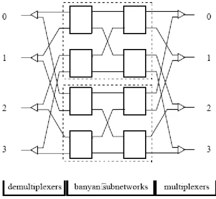
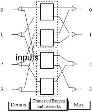
1, 2,…) parallel subnetworks. Each of these subnetworks is a banyan network. Two techniques are used to distribute the incoming cells over the R subnetworks. In the first technique, input i of the switch is connected to input i of each subnet by a 1-to-R demultiplexer. The demultiplexer forwards the incoming cells randomly across the subnetworks. Similarly, each output i of a subnet is connected to the output i of the switch through a R -to-1 multiplexer. If more than one cell arrive at the multiplexer, one of them is selected randomly to be forwarded to the output port and the others are discarded. This technique is called randomly loading parallel networks (Rn) [3]. Fig. 2.3 shows a 4x4 randomly loaded banyan network constructed from two 4x4 banyan networks. The second technique groups the outputs of the switch and assigns each group to one of R truncated subnetworks. The i th input of the switch is connected to the input of each subnet through a 1 -to-R demultiplexer. The demultiplexer forwards incoming cells according to their most significant bits of the destination address field. The outputs of each subnet, which are destined to the same switch output, are connected via a R -to-1 multiplexer to this output. This technique is called selectively loading parallel networks (Sn) [3]. A 4x4 selectively loaded parallel banyan network constructed from two 4x4 truncated banyan networks is shown in Fig. 2.4.
2.4 Plane Interconnected Parallel Network (PIPN).
The performance of banyan-based switches depends on the applied traffic. As the applied traffic becomes heterogeneous, the performance of banyan-based switches degrades drastically even if some performance enhancing techniques are employed. In [4], the PIPN, a new banyan based interconnection structure which exploits the desired properties of banyan Networks while improving the performance by alleviating their drawbacks, is introduced. In PIPN, the traffic arriving at the network is shaped and routed through two banyan network based interconnected planes. The interconnection between the planes distributes the incoming load more
homogeneously over the network. PIPN is composed of three main units, namely, the distributor, the router, and the output -port dispatcher as shown in Fig. 2.5. The cells arriving at the distributor divides the network into two groups in a random manner: the back plane and the front plane groups. The destination address fields of cells in one of the groups are complemented. The grouped cells are assigned to the router, which is a N/2 x N/2 banyan network. The cells are routed with respect to the information kept in their destination address fields. Due to the internal structure of the router and the modifications in the destination address fields of some cells, an outlet of the router may have cells actually destined to four different output ports. The cells arriving from the outlets of the router are assigned to the requested output ports in the output -port dispatcher [4]. The output-port dispatcher has two different sub-units: the decider and the collector. There is a decider unit for each router output and a collector unit for each output port. There are a total of N deciders and N collectors. The decider determines to which output port an arriving cell will be forwarded and restores its destination address field. Each collector has four inlets and internal buffer to accommodate the cells arriving from four possible deciders.
inputs outputs
Fig. 2.3. An 4x4 randomly loaded banyan network constructed form two 4x4 banyan networks
Fig. 2.4. A 4x4 selectively loaded banyan network Constructed from two 4x4 truncated banyan networks
2.4.1. The replicated PIPN switch structure
The Replicated PIPN switch applies the replication technique to the PIPN to benefit from the advantage of both techniques. Replication provides multiple paths from each input to each output pair, thus decreasing the effect of conflict between cells. PIPN gives better performance under heterogeneous traffic over the standard banyan network. A 8x8 Randomly Loaded PIPN for R=2 is shown in Fig. 2.6. It is shown from the figure that the Replicated PIPN is composed of R PIPN's connected in parallel. No multiplexers are needed at the output of the router as the deciders forward the incoming cells to the collectors’ buffers.
outputs inputs
2.5 Comment
The switch uses the replication technique to provide multiple paths between inputs and outputs and uses the PIPN to smooth the heterogeneous traffic models. The existence of more paths between each input -output ports pairs makes the modified switch more reliable than the original PIPN. As it has been shown in previous works the resulting switch has a significant increase in performance under homogeneous and heterogeneous traffic models which supports the idea of using it as a new ATM switch.
CHAPTER 3
SHARED MEDIUM FAST PACKET
SWITCH
3.1. Introduction
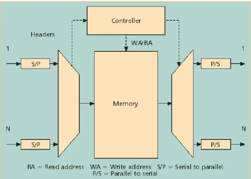
In shared medium type switches, all packets arriving on the input lines are synchronously multiplexed onto a common high –speed medium, typically a parallel bus, of bandwidth equal to N times the rate of a single input lines, where N is the number of input lines (see fig.3.1).Each output line is connected to the bus via an interface consisting of an address filter and an output FIFO buffer. Such interface is capable of receiving all packets transmitted on the bus. Depending on the packet’s virtual circuit number (or its output address), the address filter in each interface determines whether or not the packet observed in the bus to be written into the FIFO buffer. Thus, similarly to the shared- memory type, the shared- medium type switch is based on multiplexing all incoming packets into a single stream, and then demultiplexing the single stream into individual streams, one for each output line. The single path through which all packets flow here is the broadcast time-division bus and the demultiplexing is basically done by the address filters in the output interface. Conceptually, this approach is also similar to the architecture used in circuit switches based on a TDM bus, with the exception that here each packet must be processed on the fly to determine where it must be routed. The distinction between this type and the shared-memory type is that in this architecture there is complete partitioning of the memory among the output queues.
Fig.3.1.Basic structure of shared-bus type architecture
T H E D IVIS ION B U S FIFO FIFO FIFO AF AF AF P/S P/S P/S S/P S/P S/P input 1 input 2 input N output 1 output 2 output N
The shared-medium based switch has among its advocates IBM’s PARIS switch designers and NEC’s ATOM switch designers.
The PARIS switch [5], is designed for private networks. With the use of automatic network routing, the architecture of the switch can be kept very simple. Variable size packets can be accommodated, and a very efficient round robin exhaustive bus-access policy is adopted. On such a single broadcasting medium, multicasting and broadcasting functions
can easily be implemented. The ATOM switch [6], uses the bit-slice organization to alleviate the limitation of the bus speed. For still large switches, a multistage organization was proposed. Store and forward of packets, however, is needed at every stage. An alternative to the multistage organization is to use multiple shared media. Nojima et al. [7] have
developed a switch in which several shared buses are connected in matrix form with memory located at each cross point of the buses. Packets contending for access to the same bus are stored in the cross point memories connected to this bus. Arbiters scan the cross point memories and remove packets from them. In this chapter, we study a new switch architecture using multiple shared buses. This switch has the following advantages:
1) Adding input and output links without increasing the bus and I/O adaptor speed.
2) They are internally unbuffered.
3) They have a very simple control circuit.
4) They have 100% throughput under uniform traffic.
3.2.
The TDM-BASED multibus packet switch
The multi bus packet switch is designed for switching fixed size packets. The packet size can be set to 53 bytes for ATM switching.
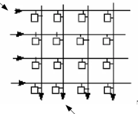
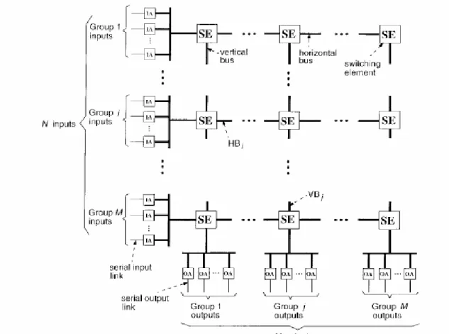
3.2.1. Architecture
Fig. 3.2 shows the architecture of an NxN multi bus packet switch. Packets enter the switch through the input links. Each input link is operated synchronously, with time being divided into link slots, where each link slot
can accommodate one packet. Each input link and each output link are connected to the switch through an input adaptor and an output adaptor, respectively. Fig. 3.3 shows the internal structure of an input and an output
serial-to-parallel conversion, and queues the packets in a set of buffers. The output adaptor performs two functions. First, it filters out all packets destined for this particular adaptor and puts them in the output buffer. Second, it performs a parallel-to-serial conversion for the packets for onward transmission.
The N input links (output links) are partitioned in M inputgroups (output groups) of L links each where N=ML. Group i input adaptors are
connected to horizontal bus HBi and group i output adaptors are connected
to vertical bus VBi . In other words, L input links are sharing a horizontal
bus, and L output links are sharing a vertical bus. The group size L here is a design parameter. If we want a smaller packet delay, each horizontal bus should serve a smaller group of input adaptors, or the group size L should be smaller. On the other hand, a larger group size L means a smaller number of groups M (for a fixed N). This means a smaller number of horizontal and vertical buses, and hence a smaller switch complexity.
The bus width is another design parameter. A larger bus width gives higher data transfer rate, and hence, a higher switch throughput at the expense of a higher implementation cost. Based on the current technology, a bus of width 64 bits operating at 100 MHz can provide a bus transfer rate of 6.4 Gbits/s.
The M horizontal buses are connected to the M vertical buses in a bus matrix, with a total of 2
M switching elements at the cross points of the
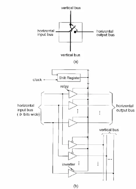
vertical and horizontal buses. The switching element placed at the cross point of HB and VB is identified as SE . Fig. 3.4(a) shows the schematic of a switching element. It connects the horizontal input bus to either the horizontal output bus or the vertical bus. Fig. 3.4(b) shows the circuit realization of the switching element, using 2b relays (b is the bus width), b
inverters, and one shift register. The relay is a three-terminal element with one input, one output, and one control line. It connects the input line to the output line whenever there is a “1” on the control line. For prototyping, the set of relays are available as off-the-shelf IC chips (e.g., Motorola’s SN54LS). For actual implementation, ASIC chips with multiple switching elements per chip can be used. Since the circuitry in each switching element is very simple, the number of switching elements per chip depends only on the number of available pins per chip.
Fig. 3.2. Multi bus packet switch.
Fig. 3.4. Switching element. (a) Schematic of the switching element and (b) circuit realization of the switching element.
For example, if the bus size is 32 bits and a chip consists of four switching elements, the chip must have 256 pins for inputs/outputs. The shift register in SE i,j stores a bit pattern which determines when to connect the
horizontal input bus to the vertical bus. When a clock pulse arrives, the last bit is shifted out to the relays. If this bit is “1,” the horizontal input bus is connected to the horizontal output bus; otherwise, the horizontal input bus is connected to the vertical bus. The connection patterns of the switching elements are chosen such that one vertical bus is connected to only one horizontal bus at a time. Note that the clock rate is equal to the packet rate
on the bus (e.g., if the bus is operated at 6 Gbits/s and the packet size is 53 bytes, the clock rate is 14.2 MHz).
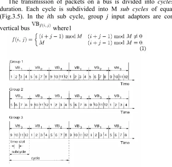
3.2.2. Operation
The transmission of packets on a bus is divided into cycles of equal
duration. Each cycle is subdivided into M sub cycles of equal duration
(Fig.3.5). In the ith sub cycle, group j input adaptors are connected to
vertical bus where1
Fig. 3.5. Transmission cycles, sub cycles, and time slots; M = 3, L = 4, and N = 12.
Thus, in the ith sub cycle, packets from group j input adaptors are switched
to group f(i,j) output adaptors. Hence, only the switching elements
SEi,f (i,j) (j=1,2,…,M) connect the horizontal buses HB to the vertical buses
VB f (i,j) (j=1,2,…,M), while all of the other switching elements connect the
horizontal input buses to the horizontal output buses. Fig. 3.5 shows an example of this transmission arrangement when M=3 and L=4. This transmission arrangement ensures that in each sub cycle, there is a unique one-to-one connection from every group of input adaptors to every group of
simultaneously transmit packets to the M groups of output adaptors through the bus matrix.
To resolve the bus contention among the L input adaptors in each group, each sub cycle is further divided into L bus slots, where each bus slot can accommodate one packet and is dedicated to one input adaptor. Each adaptor can, therefore, transmit one packet in each sub cycle. Note that when the bus transfer rate is fixed, a larger number of inputs N increase the cycle duration. Global timing is used to ensure that all transmissions are properly synchronized. This requires that all of the input adaptors and switching elements are triggered by a common clock.
3.2.2.1. Speedup Factor
We define the speedup factor SF of the switch as the ratio of the sum of
the data rates of all of the vertical buses to the sum of the data rates of all of the input links. Since there are M vertical buses and N input links, SF can be written as
Note that when SF is made larger, the buses can serve the input adaptors at a higher rate and yields a smaller input queuing delay. When SF=M, input queuing is not required, but the implementation cost is high.
3.3 Comment
This architecture looks to some extend like the pace division type, in the sense of there is a cross point that connects each input/output pair. The difference between them is that multi-bus architecture is based on cross connecting an input bus to an output bus instead of connecting an input line to an output line in space division type. The TDM multi bus architecture achieves very high through put for ATM uniform traffic, the disadvantages behind this design is that it requires a relatively high implementation cost and very robust clocking systems.
CHAPTER 4
SHARED MEMORY FAST PACKET
SWITCH
4. I. Introduction
Several different architectures are commonly used to build packet switches (e.g., IP routers, ATM switches and Ethernet switches) [8]. One well known architecture is the output-queued (OQ) switch which has the following property: When a packet arrives, it is immediately placed in a queue that is dedicated to its outgoing port, where it will wait its turn to depart. OQ switches have a number of appealing performance characteristics. First, they are work-conserving, which means that OQ switches provide 100% throughput for all types of traffic. They minimize average queuing delay, and — with the correct scheduling algorithms — can provide delay guarantees and different qualities of service. In fact, almost all of the techniques known for providing delay guarantees assume that the switch is output queued. Because of its good performance, and simple operation, several switch prototypes have emulated OQ switches using a shared medium, or a centralized shared memory. And several switch architectures proposed in the literature attempt to emulate the behavior of an OQ switch, for example Combined Input and Output Queued (CIOQ) switches [9], and Parallel Packet Switches (PPS) [10]. While each of the above techniques have their pros and cons, the shared memory architecture is the simplest technique for building an OQ switch. The block diagram of an SM ATM switch is depicted in Fig. 4.1. Early examples of commercial implementations of shared memory switches include the SBMS switching element from Hitachi [11], the RACE chipset from Siemens [12], the SMBS chipset from NTT [13], the PRELUDE switch from CNET [14], and the ISE chipset by Alcatel [15]. A shared memory switch is characterized as follows: When packets arrive at different input ports of the switch, they are written into a centralized shared buffer memory. When the time arrives for these packets to depart, they are read from this shared buffer memory and sent to the input line.
Some recent examples of commercial shared memory switches are the M40 backbone router from Juniper and the ATMS2000 chipset from MMC Networks. In general, though, there have been fewer commercially available shared memory switches than those that use other
architectures. This is because it is difficult to scale the capacity of shared memory switches to the aggregate capacity required today.
Figure .4.1 - Shared-memory ATM switch.
Why is it considered difficult to scale the capacity of shared memory switches?
Shared memory switches have the following characteristics that make it difficult to scale their capacity.
1. As the line rate R increases, the memory bandwidth of the switch’s shared memory must increase. For example, if a packet switch with N ports buffers packets in a single shared memory, then it requires a memory bandwidth of 2NR. Thus the memory bandwidth scales linearly with the line rate.
The memory bandwidth is defined here to be the reciprocal of the time taken to write data to, or read data from a random location in memory. For example, a 32-bit wide memory with a 100ns random access time is said to have a memory bandwidth of 320Mb/s.
2. If we assume that arriving packets are split into fixed sized cells of size C, then the shared memory would have to be accessed every At=C/2NR seconds. For example, if C=64 bytes, N =32 and
R=10Gb/s then the access time is just 800ps, well below the access time of SRAM (static RAM) devices, and two orders of magnitude smaller than the access time of DRAM (dynamic RAM) devices today.
3. Packet switches with faster line rates require a large shared memory. As a rule-of-thumb, the buffers in a packet switch are sized to hold approximately RTT*R bits of data (where RTT is the round trip time for flows passing through the packet switch), for those occasions when the packet switch is the bottleneck for TCP flows passing through it. If we assume an Internet RTT of
In summary, it appears that although it has attractive performance, the shared memory architecture is not scalable because of memory size and memory access time. Hence, centralized shared memory switches have
not received much attention in recent years, with research work being focused instead on input queued [16], and CIOQ switches.
4.2.
Types of Memory
It seems that neither of the currently widely available memory technologies (DRAMs and SRAMs) are well suited for use in large shared memory switches. DRAMs offer large capacity to hold many packets, but their random access time is too slow. On the other hand, SRAMs are fast and might be able to keep up with line rates, but are too small to be economically viable for large packet buffers. So we’ll consider techniques that use a combination of SRAM and DRAM, in the hope that we can find ways to combine the advantages of both, without being limited by their disadvantages. We’ll also consider techniques that use a large number of DRAMs arranged in parallel to achieve the memory bandwidth requirements. The different techniques can be broadly categorized as follows:
4.2.1. SRAM Only:
In this technique, the shared buffer memory consists of multiple (usually on-chip) SRAMs, which is ideal for low capacity switches, but does not have the storage requirements for large capacity switches because of SRAM’s low density. For example, with today’s CMOS technology, the largest available SRAM is approximately 16Mbits. If a single 16Mbit memory was used to store data flow for 0.25s (for TCP to perform well), then the aggregate capacity would be limited to less than 100Mb/s.
4.2.2. SRAM and DRAM:
Since the shared buffer memory must be capable of supporting both fast access times as well as have a large capacity, there have been several techniques proposed which use a combination of SRAM and DRAM.
The main idea is to build a memory hierarchy, where the memory bandwidth is increased by reading (writing) multiple cells from (to) DRAM memory in
parallel. When packets arrive to the switch they are segmented into cells and stored temporarily in an SRAM, waiting their turn to be written into DRAM.
At the appropriate time (determined by a memory management algorithm), multiple cells are written into the DRAMs at the same time. We can think of the memory hierarchy as a large DRAM containing a set of FIFOs.
It is common for packets to be segmented into fixed size units prior to storage. This is done for several reasons:
(1) Memory can be utilized more efficiently if all buffers are the same size.
(2) Switch fabric scheduling algorithms are often made simpler by using fixed size data units and time slots.
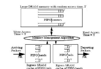
The head and tail of each FIFO is cached in a (possibly on-chip) SRAM as shown in Figure .4.2. A memory management algorithm schedules cells, manages row and bank conflicts, and inter-leaving of memory accesses. The SRAM behaves like a cache, holding packets temporarily when they first arrive and just prior to their departure. We will consider two performance metrics. First, we’ll consider the latency from when a cell is scheduled to depart until it can be retrieved from memory and placed onto the outgoing line. Bear in mind that the scheduling algorithm will schedule the cells to depart in an unpredictable order; and most likely not in the same order that they were placed into the shared memory. Ideally, the cell is always available as soon as it is scheduled. In other words, it is already available in the SRAM cache or in some other on-chip storage. As we will see, in some cases, there might instead be a bounded time (statistical bound, or hard bound) from when the cell is scheduled to depart until it is available from memory. Second, we’ll consider the size of the SRAM. A good design will require a smaller SRAM that, ideally, can be placed on-chip. The size of the SRAM depends on the types of latency guarantee made. Perhaps not surprisingly, as the guarantees become tighter, we need a larger SRAM. The approaches that use both SRAM and DRAM can be divided into two techniques.
Figure 4.2. Memory hierarchy of packet buffer, showing both DRAM and SRAM memory
4.2.2.1. Statistical Guarantees:
In this approach, the memory hierarchy gives statistical guarantees for the latency from when a cell is scheduled until it is ready to be sent on the input line. This scheme is similar to interleaving or pre-fetching used in computer systems [17]. We note however, that unlike computer systems, packet switches cannot tolerate row or bank conflicts that occasionally allow the data to be delivered at an unpredictable time. This means that when statistical guarantees are not met, data might be delivered late, out of order, or not at all.
4.2.2.2. Deterministic Guarantees
:
An alternative approach for packet switches, is to provide deterministic guarantees. Here, the SRAM is sized so that a cell is always delivered within a bounded delay, regardless of the sequence of traffic patterns, then cells are always available from memory exactly when needed.
4.2.3. DRAM Only:
The following techniques have been used to design shared memory switches using only DRAM:
4.2.3.1.
Techniques which rely on the DRAM row or bank
properties:
Here, throughput and delays are determined by the probability of row or bank conflicts. A simple technique to obtain high throughputs using DRAMs (using only random accesses) is by striping a cell across multiple DRAMs. In this approach each incoming cell is split into smaller segments and each segment is written into different DRAM banks; these banks reside over a number of parallel DRAMs. With this approach the random access time is still the bottleneck. To decrease the access time to each DRAM, cell interleaving can be used. In this technique, consecutive arriving cells are written into different DRAM banks. However since the order in which packets must depart from the shared memory switch is not known apriori, it
may happen that consecutive departing cells reside in the same DRAM row or bank, causing row or bank conflicts and momentary loss in Throughput.
4.2.3.2.
Techniques which provide statistical guarantees:
Here the memory management algorithm is designed so that the probability of DRAM row or bank conflicts is reduced. These include designs that randomly select memory locations [18], so that the probability of row or bank conflicts in DRAMs are considerably reduced. Under certain conditions, statistical bounds (such as average delay) can be found.
CHAPTER 5
OUTPUT BUFFER MANAGEMENT FOR
ATM SWITCH
5.1. Introduction
:In the shared-memory switch architecture, output links share a single large memory, in which logical FIFO queues are assigned to each link. Although memory sharing can provide a better queuing performance than physically separated buffers, it requires carefully designed buffer management schemes for a fair and robust operation. This chapter presents a survey of the buffer management methods that have been proposed for shared-memory packet switches. Several buffer management policies are described, and their strengths and weaknesses are examined. The performances of various policies are evaluated in the next chapter using computer simulations. Packet switches have another major functionality besides switching, namely, queuing. The need for queuing (also called buffering) arises since multiple cells arriving at the same time from different input lines may be destined for the same output port [1]. There are three possibilities for queuing in a packet switch: buffer cells at the input of the switch (input queuing); buffer at the output (output queuing); or buffer
internally (shared-memory). Shared-memory ATM switches gained
popularity among switch vendors due to the advantages they bring to both switching and queuing. In fact, both functions can be implemented together by controlling the memory read and write appropriately. As in output buffered switches, SM switches do not suffer from the throughput degradation caused by head of line (HOL) blocking, a phenomenon inherent in input buffered switches [19]. Moreover, modifying the memory read/write control circuit makes the SM switch flexible enough to perform functions such as priority control and multicast. Our focus is on the problem of buffer allocation. Buffer allocation determines how the total buffer space (memory) will be used by individual output ports of the switch. Our model of the SM switch is sketched from a queuing systems point of view, and is given in Fig.5.1. The switch has N output ports, and a total buffer space of M. A
first-in-first-out (FIFO) buffer is allocated to each output port, denoted by ki. The
sum of the individual buffer allocations may or may not be larger than the size of the memory M.
A certain policy of buffer allocation is required in the SM switch to perform its queuing function
Figure.5.1 - Queuing model of the shared-memory switch. i is the mean
rate of the traffic arriving at port i. ki is the size of the FIFO buffer allocated
to port i. The speed of the output link i is given by i, and the size of the
total memory space is indicated by M.
The selection and implementation of this policy is usually referred to as the buffer management. This chapter presents a survey of the research regarding the question: How should the total buffer space M of the SM
switch be managed to achieve better traffic performance (i.e., cell loss, cell delay)? Cell losses occur when a cell arrives at a switching node and finds the buffer full. Minimizing cell losses, or reducing them to acceptable levels, are extremely important to support any end-to-end application over networks.
5.2. Buffer Allocation Policies
The common goal is the analysis of possible buffer allocation policies to achieve a performance evaluation and comparison. The model in Fig.5.1 is used, and the following stochastic assumptions are made in the literature
• Packet arrivals are Poisson, i.e, they have exponentially distributed
interarrival times (with rates i, i = 1, ... , N).
• Packet lengths are exponentially distributed. Consequently, the
service time for an output link is also an exponential random variable (with mean 1/µi, i = 1, ... , N).
The output link capacities are generally assumed to be equal, i.e., µ1 = µ2 =
[20], and by Kamoun and Kleinrock [21], is called static threshold schemes
[22]. We will use the same terminology, and start with the two simplest static threshold policies: complete sharing and complete partitioning. After static threshold schemes, we will study other approaches to buffer management, such as push-out and dynamic policies.
5.2.1. Static Thresholds
5.2.1.1. Complete Partitioning and Complete Sharing
In the complete partitioning (CP) scheme, the entire buffer space is permanently partitioned among the N servers. The sum of the individual port
buffer allocations is equal to the total memory M. Hence, CP actually does
not provide any sharing. At the other extreme lies the second simple policy, complete sharing (CS). Here, an arriving packet is accepted if any space is available in the switch memory, independent of the server to which the packet is directed. In other words, individual buffer allocations equal the total memory space [21].
CS : ki = M, i = 1, ... , N (2)
where ki is the buffer allocated to port i, and M is the total buffer space. It is
possible to make a comparison intuitively by looking at the definitions above. Under the CP policy, the buffer allocated to a port is wasted if that port is inactive, since it cannot be used by other possibly active links. On the other hand, under the CS policy, one of the ports may monopolize most of the storage space if it is highly utilized [23].
The assumptions of the traffic arrival process enable us to model the switch as a Markov process. The state of the system is represented by a vector n = [n1, n2, ... , nN] where ni is the number of packets for the ith output
port. The load of link i is defined as i = i/µ.. Figure .5.2 shows the state
diagrams of CP and CS for N = 2 and M = 4. In the CS policy , a packet is
lost when the common memory is full. In CP, a packet is lost when its corresponding queue has already reached its maximum allocation.
Figure .5.2 - Markov state diagrams of CP (left) and CS (right) for a switch with two ports and a buffer space of four packets.
The assumption of exponential interarrival and service time distributions is not realistic for ATM systems. First of all, the fixed ATM cell size results in deterministic service times. Furthermore, the traffic in ATM networks is bursty in nature, implying a correlated traffic arrival process as opposed to the random traffic model presented in the earlier works [24]. A common way to model bursty traffic is by using two-state Markov chains. An on/off source, also named interrupted fluid process [24],
is a two-state Markov process that is widely used for modeling ATM traffic sources. ATM cells are only generated during the on state with fixed interarrival time. The time spent in on and off states is exponentially distributed. The model has three parameters: average length of the on period, average length of the off period, and the cell emission rate during the on period. The ratio of the on period to the sum of on and off periods is called the activity of the source, and is used as the main measure of burstiness,
although there are various other measures [25]. Although analytical methods are considered in [26], the general method is to use computer simulations for the performance evaluation of SM queuing under bursty traffic. The same approach will be taken in the next chapter to compare some of the buffer management policies presented in this chapter.