R E S E A R C H
Open Access
On the solution of high order stable time
integration methods
Owe Axelsson
1,2, Radim Blaheta
2, Stanislav Sysala
2and Bashir Ahmad
1**Correspondence:
[email protected] 1King Abdulaziz University, Jeddah, Saudi Arabia
Full list of author information is available at the end of the article
Abstract
Evolution equations arise in many important practical problems. They are frequently stiff,i.e.involves fast, mostly exponentially, decreasing and/or oscillating components. To handle such problems, one must use proper forms of implicit numerical
time-integration methods. In this paper, we consider two methods of high order of accuracy, one for parabolic problems and the other for hyperbolic type of problems. For parabolic problems, it is shown how the solution rapidly approaches the stationary solution. It is also shown how the arising quadratic polynomial algebraic systems can be solved efficiently by iteration and use of a proper preconditioner.
1 Introduction
Evolution equations arise in many important practical problems, such as for parabolic and hyperbolic partial differential equations. After application of a semi-discrete Galerkin fi-nite element or a fifi-nite difference approximation method, a system of ordinary differential equations,
Mdu
dt +Au(t) =f(t), t> ,u() =u,
arises. Here,u,f∈ n,Mis a mass matrix andM,Aaren×nmatrices. For a finite differ-ence approximation,M=I, the identity matrix.
In the above applications, the ordernof the system can be very large. Under reasonable assumptions of the given source functionf, the system is stable,i.e.its solution is bounded for allt> and converges to a fixed stationary solution ast→, independent of the initial valueu. This holds ifAis a normal matrix, that is, has a complete eigenvector space, and has eigenvalues with positive real parts. This condition holds for parabolic problems, where the eigenvalues ofAare real and positive. In more involved problems, the matrixA may have complex eigenvalues with arbitrary large imaginary parts.
Clearly, not all numerical time-integration methods preserve the above stability proper-ties. Unless the time-step is sufficiently small, explicit time-integration methods do not converge and/or give unphysical oscillations in the numerical solution. Even with suf-ficiently small time-steps, algebraic errors may increase unboundedly due to the large number of time-steps. The simplest example where the stability holds is the Euler implicit method,
˜
u(t+τ) +τAu˜(t+τ) =u˜(t) +τf(t+τ), t=τ, τ, . . . ,u˜() =u˜,
whereτ> is the time-step. Here, the eigenvalues of the inverse of the resulting matrix in the corresponding system,
(I+τA)u˜(t+τ) =u˜(t) +τf(t+τ)
equal ( +τ λ)–and satisfy the stability condition,
μ(λ)=( +τ λ)–< , λ∈σ(A).
Here,σ(A) denotes the set of eigenvalues ofA. To more quickly damp out initial transients in the solution, which arises for instance due to that the initial value may not satisfy bound-ary conditions given in the parabolic problem, one should preferably have eigenvalues of the inverse of the discrete matrixB, that satisfies|μ(λ)| → for eigenvaluesλ→ ∞. This holds for the implicit Euler method, where
B=I+τA and μ(λ) = ( +τ λ)–.
This method is only first-order accurate,i.e.its global time discretization error isO(τ). Therefore, to get a sufficiently small discretization error, one must choose very small time-steps, which means that the method becomes computationally expensive and also causes a stronger increase of round-off errors. However, there exists stable time-integration meth-ods of arbitrary high order. They are of implicit Runge-Kutta quadrature type (see e.g. [–]), and belong to the class ofA-stable methods,i.e.the eigenvaluesμ(B–) of the cor-responding matrixBwhereBu˜(t+τ) =u˜(t) +τ˜f(t), and˜f(t) is a linear function off(t) at the quadrature points in the interval [t,t+τ], satisfy|μ(B–)|< for all normal matrices M–Awithe(λ) > . The highest order achieved,O(τm) occurs for Gauss quadrature wheremequals to the number of quadrature points within each time interval.
To satisfy the second, desirable condition,
lim
λ→∞
μ(λ)→,
one can use a special subclass of such methods, based on Radau quadrature; see,e.g.[, ]. The discretization error is here only one order less,O(τm–). For linear problems, all such stable methods lead to rational polynomial approximation matricesB, and hence the need to solve quadratic polynomial equations. For stable methods, it turns out that the roots of these polynomials are complex.
In Section , a preconditioning method is described that is very efficient when solving such systems, without the need to factorize the quadratic polynomials in first order fac-tors, thereby avoiding the need to use complex arithmetics. Section discusses the special case wherem= . It shows also how the general case, wherem> , can be handled.
Section deals with the use of implicit Runge-Kutta methods of Gauss quadrature type for solving hyperbolic systems of Hamiltonian type.
Section presents a method to derive time discretization errors.
2 Preconditioners for quadratic matrix polynomials
From the introduction, it follows that it is of importance to use an efficient solution method for quadratic matrix polynomials and not factorize them in first order factors when this results in complex valued factors. For a method to solve complex valued systems in real arithmetics, see,e.g.[]. Here, we use a particular method that is suitable for the arising quadratic matrix polynomials.
Consider then the matrix polynomial,
B=M+aA+bAM–A. ()
We assume thatMis spd and that|a|< b, which latter implies that the first order factors ofBare complex. Systems withBwill be solved by iteration. As a preconditioner, we use the matrix
Cα= (M+αA)M–(M+αA),
whereα> is a parameter. We assume thatAis a normal matrix, that is, has a full eigen-vector space and further that the symmetric part,A+AT ofAis spd. To estimate the eigenvalues ofC–
α B, we write
(Cαx,x) – (Bx,x) = (α–a)(Ax,x) +
α–bAM–Ax,x.
After a two-sided multiplication withM–/, we get
(C˜αx˜,x˜) – (B˜x˜,x˜) = (α–a)(A˜x˜,x˜) +
α–bA˜x˜,x˜, ()
whereC˜α=M–/CαM–/= (I+αA˜),etc.andx˜=M/x. Note that, by similarity,Cα–B andC˜–
α B˜ have the same eigenvalues.
We are interested in cases whereA˜ may have large eigenvalues. (In our application,A˜ involves a time-step factorτ, but since we use higher order time-discretization methods, τ will not be very small and cannot damp out the inverse to some power of the space-discretization parameterhthat also occurs inA˜.) Therefore, we chooseα=b. Note that this implies that α–a> .
The resulting relation () can now be written
(x˜,x˜) –C˜–α B˜x˜,x˜
= (α–a)C˜–α A˜x˜,x˜
, ()
where
˜ Cα–A˜x˜,x˜
=(I+αA˜)–A˜x˜,x˜.
Since α–a> , the real part of the eigenvalues ofC˜α–B˜ are bounded above by . To find estimates of the eigenvaluesλ(μ) ofC˜–
α B˜, let (μ,z) be eigensolutions ofA˜,i.e.let
˜
It follows from () that forx˜=z,
λ(μ) =C˜α–B˜z,z
= –
– a α
αμ + αμ+ (αμ)
= –
– a α
+
(αμ+ αμ)
.
We writeαμ=μeiϕso (αμ+αμ ) = (μ+
μ)cos(ϕ) +
i (μ–
μ)sin(ϕ), whereiis the
imaginary unit. Note thatμ> so(μ+μ)≥. Since, by assumption, the real part of μis positive, it holds|ϕ| ≤ϕ<π/. A computation shows that the values of the factor
+(αμ+αμ) are located in a disc in the complex plane with center atδ/ and radiusδ/, whereδ= /( +cosϕ).
Hence,λ(μ) is located in a disc with center at –( –aα)δand radius( –aα)δ. Forϕ= ,i.e.for real eigenvalues ofA˜, thenδ= / and ≥λ(μ)≥+aα.
3 A stiffly stable time integration method
Consider a system of ordinary differential equations,
Mdx dt +σ(t)
Ax(t) –f(t)= , t> ,x() =x, ()
wherex,f∈ n,σ(t)≥σ> ,M,Aaren×nmatrices, whereMis assumed to be spd and the symmetric part ofAis positive semidefinite. In the practical applications that we consider,Mcorresponds to a mass matrix andAto a second-order diffusion or diffusion-convection matrix. Hence,nis large. Under reasonable assumptions on the source func-tionf, such a system is stable for alltand its solution approaches a finite function, inde-pendent on the initial valuex, ast→ ∞.
Such stability results hold for more general problems, such as for a nonlinear parabolic problem,
∂u
∂t +F(t,u) = , whereF(t,u) = –∇ ·
a(t,u,∇u)∇u–f(t,u),x∈,t> , ()
wheref : (,∞)×V→V andV is a reflexive Banach space. For proper functionsa(·) andf(·), thenFis monotone,i.e.
F(t,u) –F(t,v),u–v≥ρ(t)u–v, ∀u,v∈V,t> . ()
Here, ρ: (,∞)→R, ρ(t)≥ and (·,·), · denote the scalar product, and the corre-sponding norm inL(), respectively. In this case, one can easily derive the bound
d dt
u–v= –F(t,u) –F(t,v),u–v≤–ρ(t)u–v,
whereu,vare solution of () corresponding to different initial values. Consequently mak-ing use of the Gronwall lemma, we obtain
u(t) –v(t)≤exp
–
t
ρ(s)dsu() –v()≤u() –v(), t> .
IfFis strongly monotone (or dissipative),i.e.() is valid withρ(t)≥> , then
u(t) –v(t)≤exp(–tρ)u() –v()→, t→ ∞,
i.e.() is asymptotically stable. In particular, the above holds for the test problem consid-ered in Section .
For large eigenvalues ofM–A, such a system is stiff and can have fast decreasing and possibly oscillating components. This amounts to that the eigenvalues have large real part and possibly also large imaginary parts. To handle this, one needs stable numerical time-integration methods that do not contain corresponding increasing components. For σ(t) = , in (), this amounts to proper approximations of the matrix exponential function
exp(tE),E=M–A, by a rational function,
Rm(tE) =Qm(tE)–Pm(tE),
where
Rm(tE)≤, t> , forRe{λE}> ,
andλEdenotes eigenvalues byE. Furthermore, to cope with problems wherearg(λE)≤α< π
, but arbitrarily close toπ/, one needsA-stable methods; seee.g.[, , ]. To get stability for all times and time steps, one requireslim|λ|→∞|Rm(λ)| ≤c< where preferablyc= . Such methods are calledL-stable (Lambert) and stifflyA-stable [], respectively.
An important class of methods which are stifflyA-stable is a particular class of the im-plicit Runga-Kutta methods; see [, , ]. Such methods correspond to rational polynomial approximations of the matrix exponential function with denominator having a higher de-gree than the nominator. Examples of such methods are based on Radau quadrature where the quadrature points are zeros ofP˜m(ξ) –P˜m–(ξ), where{˜Pk}are the Legendre polyno-mials, orthogonal on the interval (, ), seee.g.[] and references therein. Note thatξ= is a root for allm≥. The casem= is identical to the implicit Euler method.
Following [], we consider here the next simplest case, wherem= , for the numerical solution of () over a time interval [t,t+τ].
In this case, the quadrature points (for a unit interval) areξ= /,ξ= and the nu-merical solutionx,x, att+τ/ andt+τ satisfies
M+ σA˜ –σA˜ σA˜ M+ σA˜
x
x
= Mx+ τ
(f–f) Mx+τ(f+f)
, ()
wherexis the solution at timet,σ=σ(t+τ/),σ=σ(t+τ),f=f(t+τ/),f=f(t+τ), andA˜ = τ
A. The global discretization error of thex-component for this method isO(τ), i.e.it is a third-order method and it is stifflyA-stable even for arbitrary strong variations of the coefficientσ(t). This can be compared with the trapezoidal or implicit midpoint methods which are only second order accurate and not stiffly stable.
that involves only an inner system with matrixM–. To this end, but only for the derivation of the method, we scale first the system with the block diagonal matrixM–
M–
to get
I+ σG –σG σG I+ σG
x
x
= x+ τ
(˜f–f˜)
x+τ(f˜+f˜)
,
whereG=τM–Aand˜f
i=M–fi,i= , . The Schur complement system forxis multi-plied with (I+ σG). Using commutativity, we get then
(I+ σG)(I+ σG) + σσG
x
= (I+ σG)
x+ τ
(f˜+˜f)
– σG
x+ τ
(f˜–˜f)
or
I+ (σ+ σ)G+ σσG
x
= (I– σG)x+ τ
(f˜+˜f) + τ σG˜f.
Hence,
Bx=
M–τ σA
x+ τ
M(f˜+f˜) + τ
σ A˜f,
where
B=M+ τ
(σ+ σ)A+ τ
σσAM
–A. ()
For higher order Radau quadrature methods, the corresponding matrix polynomial in M–Bis amth order polynomial. By the fundamental theorem of algebra, one can fac-torize it in factors of at most second degree. They can be solved in a sequential order. Alternatively, using a method referred to in Remark ., the solution components can be computed concurrently.
Each second-order factor can be preconditioned by the method in Section . The ability to factorizeQm(tE) in second-order factors and solve the arising systems as such two-by-two block matrix systems means that one only has to solve first-order systems. This is of importance if for instanceMandAare large sparse bandmatrices, since then one avoids increasing bandwidths in matrix products and one can solve systems of linear combina-tions ofMandAmore efficiently than for higher order polynomial combinations. Fur-thermore, this enables one to keep matrices on element by element form (see,e.g.[]) and it is in general not necessary to store the matricesMandA. The arising inner system can be solved by some inner iteration method.
The problem with a direct factorization in first order factors is that complex matrix factors appear. This occurs for the matrix in () for a ratio of σ
σ in the interval
– √ < σ σ
< +
√
Therefore, it is more efficient to keep the second order factors and instead solve the corre-sponding systems by preconditioned iterations. Thereby, the preconditioner involves only first order factors. As shown in Section , a very efficient preconditioner for the matrixB in () is
C=Cα= (M+ατA)M–(M+σ τA), ()
whereα> is a parameter. As already shown in [], for the above particular application it holds.
Proposition . Let B,C be as defined in()and()and assume that M is spd and A is spsd.Then letting
α=maxσσ/, (σ+ σ)/
it holds
κC–B≤max
i=,δ – i ,
where
≥δ= (σ+ σ)/α≥
√
/,
≥δ=σσ/α.
If.≤σ
σ ≤.,thenδ= andδ≥
. The spectral condition number is then bounded by
κC–B≤
≈..
Ifσ=σ,then
κC–B≤
≈..
Proof Let (u,v) be theproduct ofu,v∈ n. We have
(Cx,x) – (Bx,x) = σ τ( –δ)(Ax,x) +ατ( –δ)
AM–Ax,x ∀x∈ n.
It follows that
(Bx,x)≤(Cx,x).
By the arithmetic-geometric means inequality, we have
δ≥
σσ/α≥
√
√
=
√
a computation shows that
σσ/≥
σ+ σ
for .ξ., whereξ=σ/σ. Further, a computation shows thatδ≥
, which is in accordance with the lower bound in (). Since
(Cx,x)≥ατ(Ax,x) +ατAM–Ax,x,
it follows that
– (Bx,x) (Cx,x)≥ –δ
or
(Bx,x) (Cx,x)≤δ=
.
Forα=α, a computation shows that
δ=
√
=
.
We conclude that the condition number is very close to its ideal unit value , leading to very few iterations. For instance, it suffices with at most conjugate gradient iterations for a relative accuracy of –.
Remark . High order implicit Runge-Kutta methods and their discretization error es-timates can be derived using order tree methods as described in [] and [].
For an early presentation of implicit Runge-Kutta methods, see [] and also [], where the method was called global integration method to indicate its capability for large val-ues ofmto use few, or even just one, time discretization steps. It was also shown that the coefficient matrix, formed by the quadrature coefficients had a dominating lower trian-gular part, enabling the use of a matrix splitting and Richardson iteration method. It can be of interest to point out that the Radau method form= can be described in an alter-native way, using Radau quadrature for the whole time step interval and combined with a trapezoidal method for the shorter interval.
Namely, letdudt +f(t,u) = ,tk–<t<tk. Then Radau quadrature on the interval (tk–,tk) has quadrature pointstk–+τ/,tk, and coefficientsb= /,b= /, which results in the relation
˜
u–u˜ +τ
f(˜t/,u/˜ ) + τ
f(t˜,u˜ ) = ,
This equation is coupled with an equation based on quadrature
u(tk–+τ/) –u(tk–) + tk
tk–
f(t,u)dt– tk
tk–+τ/
f(t,u)dt= ,
which, using the stated quadrature rules, results in
˜
u/–u˜ +τ
f(˜t/,u/˜ ) + τ
f(t˜,u˜ ) –
τ
f(˜t/,u/˜ ) +f(˜t,u˜ )=
that is,
˜
u/–u˜ +τ
f(˜t/,u/˜ ) – τ
f(˜t,u˜ ) = .
Remark . The arising system in a high order method involvingq≥ quadratic poly-nomial factors, can be solved sequentially in the order they appear. Alternatively (see,e.g. [], Exercise .), one can use a method based on solving a matrix polynomial equa-tion,Pq(A)x=basx=
q k=
Pq(rk)xk,xk= (A–rkI)
–b, where{r
k}q, is the set of zeros of the polynomial and it is assumed thatAhas no eigenvalues in this set. (This holds in our applications.) Then, combining pairs of terms corresponding to complex conjugate rootsrk, quadratic polynomials arise for the computation of the corresponding solution components. It is seen that in this method, the solution components can be computed concurrently.
Remark . Differential algebraic equations (DAE) arise in many important problems; see, for instance [, ]. The simplest example of a DAE takes the form
⎧ ⎨ ⎩
du
dt =f(t,u,v), g(t,u,v) = , t> ,
withu() =u,v() =vand it is normally assumed that the initial values satisfy the con-straint equation,i.e.
g(,u,v) = .
Ifdet(∂g∂v)= in a sufficiently large set around the solution, one can formally eliminate the second part of the solution to form a differential equation in standard form.
du dt =f
t,u,v(u), t> ,u() =u.
Such a DAE is said to have index one, seee.g.[]. It can be seen to be a limit case of the system
⎧ ⎨ ⎩
du
dt =f(t,u,v), du
dt =
εg(t,u,v),
Hence, such an DAE can be considered as an infinitely stiff differential equation problem. For strongly or infinitely stiff problems, there can occur an order reduction phenomenae. This follows since some high order error terms in the error expansion (cf.Section ) are multiplied with (infinitely) large factors, leading to an order reduction for some methods. Heuristically, this can be understood to occur for the Gauss integration form of IRK but does not occur for the stiffly stable variants, such as based on the Radau quadrature. For further discussions of this, see,e.g.[, ].
4 High order integration methods for Hamiltonian systems
Another important application of high order time integration methods occurs for Hamil-tonian systems. Such systems occur in mechanics and particle physics, for instance. As an introduction, consider the conservation of energy principle. To this end, consider a mechanical system ofkpoint masses and its associated Lagrangian functional,
L=K–V= k
i= mi|˙xi|
–V(x
, . . . ,xk),
whereKis the kinetic energy andVthe potential energy. Here,xi= (xi,yi,zi) denote the Cartesian coordinate of theith point massmi.
The configuration strives to minimize the total energy. The corresponding Euler-Lagrange equations become then ∂L
∂xi = , that is,
mix¨i= – ∂V ∂xi
, i= , , . . . ,k. ()
We consider conservative systems,i.e.mechanical systems for which the total force on the elements of the system are related to the potentialV:k⇒ according to
Fi= – ∂V ∂xi .
This means that the Euler-Lagrange equation () is identical to the classical Newton’s law
mix¨i=Fi, i= , , . . . ,k.
Letpi=mivibe the momentum. Then
K= k
p i mi
.
A mechanical system can be described by general coordinates
q= (q, . . . ,qd)
i.e.not necessarily Cartesian, but angles, length along a curve,etc.The Lagrangian takes the formL(q,q˙,t). Ifqis determined to satisfy
min
q b
a
then the motion of the system is described by the Lagrange equation,
d dt
∂L
∂q˙(q,q˙,t) =
∂L
∂q(q,q˙,t). ()
Letting here
pk= ∂L ∂q˙k
(q,q˙), k= , . . . ,n
be the momentum variable, and using the transformation (q,q˙) = (q,p) we can write () as the Hamiltonian,
H(p,q,t) = n
j=
pjq˙j–L
q,q˙(q,p,t),t.
For a mechanical system with potential energy a function of configuration only and ki-netic energyKgiven by a quadratic form
K= q˙
TG(q)q˙,
whereGis an spd matrix, possibly depending onq, we get
p=G(q)q˙, q˙=G–(q)p ()
and
H(p,q,t) =pTG–(q)p– p
TG–(q)p+V(q)
= p
TG–(q)p+V(q) =K(p,q) +V(q),
which equals the total energy of the system.
The corresponding Euler-Lagrange equations become now ⎧
⎨ ⎩
˙ p= –∂H∂q,
˙
q=∂H∂p ()
and are referred to as the Hamiltonian system. This follows from
∂H ∂p =q˙
T+pT∂q˙ ∂p–
∂L ∂q˙
∂q˙
∂p=q˙ T,
∂H ∂q =p
T∂q˙ ∂q –
∂L ∂q–
∂L ∂q˙
∂q˙
∂q= –
∂L ∂q,
which, sincedtd(∂L∂q˙) = ∂∂Lqimpliesp˙=∂L∂q, are hence equivalent to the Lagrange equations. By (), it holds
d
dtH(p,q) = ∂H
∂pp˙+
∂H
∂qq˙= , ()
The flowϕt:U→ nof a Hamiltonian system is the mapping that describes the evo-lution of the soevo-lution by time,i.e.ϕt(p,q) = (p(t,p,q),q(t,p,q)), wherep(t,p,q),
q(t,p,q) is the solution of the system for the initial valuesp() =p,q() =q. We consider now a Hamiltonian with a quadratic first integral in the form
H(y) =yTCy, y= (p,q), ()
whereCis a symmetric matrix. For the solution of the Hamiltonian system (), we shall use an implicit Runge-Kutta method based on Gauss quadrature.
Thes-stage Runge-Kutta method applied to an initial value problem,y˙=f(t,y),y(t) =
yis defined by
⎧ ⎨ ⎩
ki=f(t+ciτ,y+τ s
j=aijkj), i= , , . . . ,s, y=y+τsi=biki,
()
whereci= s
i=aij, seee.g.[, ]. The familiar implicit midpoint rule is the special case where s= . Here,c, . . . ,cs are the zeros of the shifted Legendre polynomial d
s
dxs(xs( –
x)s). For a linear problem, this results in a system which can be solved by the quadratic polynomial decomposition and the preconditioned iterative solution method, presented in Section .
Ifu(t) is a polynomial of degree s, then () takes the form
u(t) =y,
˙
u(t+ciτ) =f
t+cτ,y(t+ciτ)
, i= , . . . ,s
()
andu=u(t+τ).
For the Hamiltonian (), it holds
d dtH
y(t)= yT(t)Cy(t)
and it follows from () that
yTCy–yTCy= t+τ
t
u(t)TCu˙(t)dt.
Since the integrand is a polynomial of degree s– , it is evaluated exactly by thes-stage Gaussian quadrature formula. Therefore, since
y(t+cit)TC˙y(t+ciτ) =u(t+ciτ)TCf
u(t+ciτ)
=
it follows that the energy quadrature formsyT
iCiyiare conserved.
5 Discretization error estimates
Error estimation methods for parabolic and hyperbolic problems can differ greatly. Parabolic problems are characterized by the monotonicity property () while for hyper-bolic problems a corresponding conservation property,
F(t,u) –F(t,v),u–v= , t> ∀u,v∈V
holds, implying
u(t) –v(t)=u() –v(), t≥. ()
Hence, there is no decrease of errors occurring at earlier time steps. On the other hand, the strong monotonicity property for parabolic problems implies that errors at earlier time steps decrease exponentially as time evolves.
For a derivation of discretization errors for such parabolic type problems for a convex combination of the implicit Euler method and the midpoint method, referred to as the θ-method, the following holds (see []). Similar estimates can also be derived for the Radau quadrature method, see,e.g.[].
The major result in [] is the following. Letus
t= ∂s(u(t))
∂ts . Consider the problemut=F(t,u(t)) whereubelongs to some function
spaceV and the corresponding truncation error,
Rθ(t,u) =Ft¯,u¯(t)–τ– t+τ
t
ut(s)ds
=u(¯t) –τ–u(t+τ) –u(t)+F¯t,u¯(t)–F¯t,u(¯t),
where¯t=θt+ ( –θ)(t+τ),u¯(t) =θu(t) + ( –θ)u(t+τ), ≤θ≤. Ifu∈C(V), then a Taylor expansion shows that
Rθ(t,u) = – τ
u() t (t) +
–θ
τu()t (t)
+
θ( –θ)τ ∂F
∂y
t,u˜(¯t)u()t (t), t<ti<t+τ,i= , , , ()
whereu˜(t) takes values in a tube with radiusu(t) –u(t)about the solutionu(t). It follows that if
∂F
∂u
t,u˜(t)u()t
t(t)≤C ()
andθ=–O(τ), then
Rθ(t,u)=Oτ.
Under the above conditions, the discretization errore(t) =u(t) –v(t), where
v(t+τ) –v(t) +τFt,v(t)= , t= ,τ, τ, . . . ,
(i) ifFis strongly monotone and–|O(τ)| ≤θ≤θ, thene(t) ≤–Cτ,t> ; (ii) ifFis monotone (or conservative) and–|O(τ)| ≤θ≤, thene(t) ≤tCτ,t> . Here,C depends onu()t andu()t , but is independent of the stiffness of the problem under the appropriate conditions stated above.
If the solutionuis smooth so that∂F∂uu()t has also only smooth components, then∂F∂uu () t may be much smaller than∂F∂uu()t , showing that the stiffness,i.e.factors∂F∂u , do not enter in the error estimate.
In many problems, we can expect that∂F∂uu()t is of the same order asu()t ,i.e.the first and last forms in () have the same order. In particular, this holds for a linear problem ut+Au= , whereu()t =Au=∂F∂uu
() t .
It is seen from () that for hyperbolic (conservative) problems like the Hamiltonian problem in Section , the discretization error grows at least linearly witht, but likely faster if the solution is not sufficiently smooth. It may then be necessary to control the error by coupling the numerical time-integration method with an adaptive time step control. We present here such a method based on the use of backward integration at each time-step using the adjoint operator. The use of adjoint operators in error estimates gives back to the classical Aubin-NitscheL-lifting method used in boundary value problems to derive discretization error estimates inLnorm. It has also been used for error estimates in initial value problems, seee.g.[].
Assume that the monotonicity assumption () holds. We show first a nonlinear (mono-tone) stability property, calledB-stability, that holds for the numerical solution of implicit Runge-Kutta methods based on Gauss quadrature points. It goes back to a scientific note in []; see also [].
Letu˜,v˜be two approximate solutions tou =f(u,t),t> extended to polynomials of degreemfrom their pointwise values attk,iin the interval [tk–,tk]. Let
(t) =
u˜(t) –v˜(t)
.
Then, since by (),u˜(t) andv˜(t) satisfy the differential equation at the quadrature points, and by () it holds
(tk,i) =
˜
u(tk,i) –v˜(tk,i),u˜(tk,i) –v˜(tk,i)
=fu˜(tk,i)
–fv˜(tk,i)
,u˜(tk,i) –v˜(tk,i)
≤,
i= , , . . . ,m, where{tk,i}mi=is the set of quadrature points. Since(t) is a polynomial of degree m– , Gauss quadrature is exact so
(tk) –(tk–) = tk
tk–
(s)ds= m
i=
bi(tk,i)≤.
Here,bi> are the quadrature coefficients. Hence,
u˜(tk) –v˜(tk)≤u˜(tk–) –v˜(tk–)≤ · · · ≤u˜() –v˜(), k= , , . . . .
We present now a method for adaptive a posteriori error control for the initial value problem
u(t) =σ(t)fu(t), t> ,
u() =u,
()
whereu(t)∈Rnandf(u(t)) =Au(t) –f˜(t).
For the implicit Runge-Kutta method with approximate solutionu˜(t), it holds
˜
u(tk) =u˜(tk–) + tk
tk–
σ(t)fu˜(t)dt, k= , ,
whereu˜(t) is a piecewise polynomial of degreem. The corresponding residual equals
Ru˜(t)=u˜(t) –σ(t)fu˜(t).
By the property of implicit Runge-Kutta methods, it is orthogonal,i.e.
tk
tk–
˜
u(t) –σ(t)fu˜(t)·v dt= , k= , , . . . ()
to all polynomials of degreem. Here, the ‘dot’ indicates a vector product inRn. The dis-cretization error equalse(t) =u(t) –u˜(t),t> . The error estimation will be based on the backward integration of the adjoint operator problem,
⎧ ⎨ ⎩
ϕ(t) = –σ(t)ATϕ(t), tk–<t<tk,
ϕ(tk) =e(tk). ()
Note thatσ(t)Ae(t) =σ(t)(f(u(t)) –f(u˜(t))). It holds
e(tk)
=e(tk)+ tk
tk–
e·–ϕ –σ(t)ATϕdt,
so by integration by parts, we get
e(tk)= tk
tk–
e –σ(t)Ae·ϕdt+e(tk–)·ϕ(tk–).
Here
e –σ(t)Ae=u –σ(t)Au–f˜(t)–u˜ –σ(t)Au˜–f˜(t)= –u˜ +σ(t)f(u˜) = –R(u˜).
Hence,
e(tk)= – tk
tk–
Here, we can use the Galerkin orthogonality property () to get
e(tk)–e(tk–)·ϕ(tk–)≤min
˜
ϕ ttk
k–
R(u˜)·(ϕ–ϕ˜)dt,
whereϕ˜is a polynomial of degreem. Sinceϕ(tk) =e(tk), it follows that
e(tk)≤ϕ(tk–) ϕ(tk)
e(tk–)+min
˜
ϕ tk
tk–
R(u˜)ϕ–ϕ˜ ϕ(tk) dt
,
and fromϕ(t) = –σ(t)ATϕ(t) andμ(AT) =μ(A) =max
iRe|λi(A)|= , it follows that
ϕ(t) =e
tk
t μ(t)σ(t)dtϕ(tk) =ϕ(tk).
Hence,
e(tk)≤e(tk–)+min
˜
ϕ tk
tk–
R(u˜)ϕ–ϕ˜ ϕ(tk) dt
.
Under sufficient regularity assumptions the last term can be bounded byCτm. Hence, the discretization error grows linearly with time,
e(tk)≤Ctkτm, k= , , . . .
i.e.the implicit Runge-Kutta method, based on Gaussian quadrature, applied for hyper-bolic (conservative) problems has order m.
6 A numerical test example
We consider the linear parabolic problem,
∂u
∂t +σ(t)(–u+b· ∇u–f) = , t> ()
in the unit square domain= [, ]with boundary condition ⎧
⎨ ⎩
u= on partsy= ,y= , ∂u
∂ν +u=g,≥ on partsx= ,x= .
()
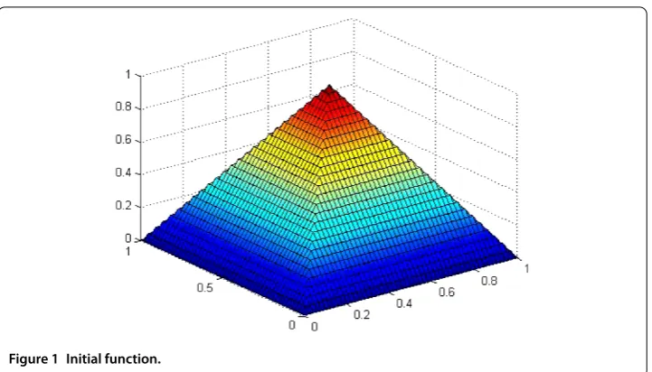
As initial functionu, we choose a tent-like function withu= at the center ofand u= on∂; see Figure .
Here,σ(t) = +sinkπt, wherek= , , . . . ,k≤τ, is a parameter used to test the stability of the method with respect to oscillating coefficients. Here,τ is the time step to be used in the numerical solution of (). Note that this functionσ(t) satisfies the conditions of the ratio σ
σ from (). We letf(x,y)≡e
–x.
Figure 1 Initial function.
After a finite element or finite difference approximation, a system of the form () arises. For a finite difference approximationM=I, the identity matrix. The Laplacian operator is approximated with a nine-point difference scheme. We use an upwind discretization of the convection term. In the outer corner points of the domain, we use the boundary conditions –ux+u= forx= andux+u= forx= .
The time discretization is given by the implicit Runge-Kutta method with the Radau quadrature for m= ; see Section . For comparison, we also considerm= ,i.e. the implicit Euler method, in some experiments. For solving the time-discretized problems, we use the GMRES method with preconditioners from Section and with the tolerance e– . Let us note that GMRES needs - iteration for this tolerance. The problem is implemented in Matlab.
The primary aim is to show how the time-discretization errors decrease and how fast the numerical approximation of ()-() approaches its stationary value,i.e.the corre-sponding numerical solution to the stationary problem
⎧ ⎪ ⎪ ⎨ ⎪ ⎪ ⎩
–uˆ+b· ∇ ˆu= e–x in,
u= on partsy= ,y= , ∂u
∂ν +u=g on partsx= ,x= .
()
6.1 Experiments with a known and smooth stationary solution
If we let
g(y) = ⎧ ⎨ ⎩
y( –y) forx= ,
forx=
then the solution to () satisfies
ˆ
Table 1 The error estimates in dependence onandh
\h 1/10 1/20 1/50 1/100 1/150
1 1.2e–2 5.9e–3 2.3e–3 1.2e–3 7.7e–4 20 6.1e–1 4.5e–1 2.5e–1 1.4e–1 9.4e–2
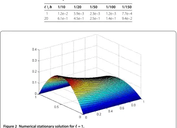
Figure 2 Numerical stationary solution for= 1.
First, we will investigate the influence of the space discretization error on the stationary problem (). To this end, we use the relative error estimate in the Euclidean norm:
eh=
ˆuh–uˆ
ˆu .
Here,uˆ,uˆh denote the vectors representing the exact and numerical solutions to () at the nodal points, respectively. The error estimates in dependence onandhare found in Table . It is seen that the error decay isO(h). This is caused by the use of first order upwind approximation of the convection term.
In Figures and , there are depicted numerical stationary solutions for= and= , respectively. The discretization parameter ish= /.
Now we will investigate how fast the numerical solution to ()-() approaches the numerical solution to () in dependence onτ. We fixk= and we search the smallest timeTfor which
uh(T) –uˆh
ˆuh
< –,
where the vectorsuˆhanduh(T) represent the numerical solution to () and the numerical solution to ()-() at timeT, respectively. The results for variousandhare in Table . We can observe that the dependence of the results onhis small. For smaller, the final time does not depend onτ, while for larger, the dependence onτ is more significant.
max-Figure 3 Numerical stationary solution for= 20.
Table 2 Values of timeTin dependence onhandτ
h\τ 1/5 1/10 1/20 1/40
1/20 1.40 1.30 1.25 1.25 1/50 1.40 1.30 1.25 1.25
h\τ 1/5 1/10 1/20 1/40
1/20 1.40 0.70 0.35 0.18 1/50 1.60 0.80 0.40 0.18
We use= 1(left) and= 20(right).
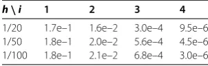
Table 3 Time discretization error at timeT= 1/8 in dependence onhandτ
h\i 1 2 3 4
1/20 1.7e–1 1.6e–2 3.0e–4 9.5e–6 1/50 1.8e–1 2.0e–2 5.6e–4 4.5e–6 1/100 1.8e–1 2.1e–2 6.8e–4 3.0e–6
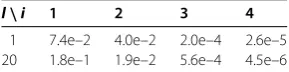
Table 4 Time discretization error at timeT= 1/8 in dependence onandτ
\i 1 2 3 4
1 7.1e–2 3.9e–3 2.1e–4 2.8e–5 20 1.8e–1 2.0e–2 5.6e–4 4.5e–6
Table 5 Time discretization error at timeT= 1/8 in dependence onkandτ
k\i 1 2 3 4
0 1.1e–1 2.4e–2 4.3e–4 2.4e–5 10 1.8e–1 2.0e–2 5.6e–4 4.5e–6
imal differences between the vectorsui(T) andui+(T),i= , . . . , , whereui(T) represents
the numerical solution to ()-() at time T for the time-discretization parameterτi, i= , . . . , . So, we investigate the following error:
ei=ui+(T) –ui(T)∞, i= , . . . , ,
Table 6 Time discretization error at timeT= 1/8 in dependence onandτfor the implicit Euler method
k\i 1 2 3 4
0 7.8e–2 4.2e–2 1.7e–2 4.6e–3 10 2.5e–2 2.5e–2 4.8e–2 2.2e–2
Table 7 Values of stabilized timeTin dependence onandτ
\τ 1/5 1/10 1/20 1/40
1 1.40 1.30 1.25 1.23 20 1.60 0.80 0.45 0.20
We leth= 1/50.
Table 8 Time discretization error at timeT= 1/8 in dependence onandτ
l\i 1 2 3 4
1 7.4e–2 4.0e–2 2.0e–4 2.6e–5 20 1.8e–1 1.9e–2 5.6e–4 4.5e–6
is small for the larger time steps but more noticeable for the smaller time steps when the time and space discretization errors are of the same order.
If we letk= ,h= /,= and= , we obtain results in Table . We can see that the investigated time-discretization error decreases faster for= than for= .
If we letk= ,k= ,h= /, and= , we obtain results in Table .
The error estimates from Tables - indicate that the expected error estimateO(τ) holds.
For comparison, we perform the same experiment as in Table for the implicit Euler time discretization. The results are in Table .
The error estimates are here significantly influenced by the oscillation parameterk. For the larger valuek= , we do not observe convergence. In casek= , the convergence is first orderO(τ), that is, much slower than for the Runge-Kutta method with the two-point Radau quadrature.
6.2 Experiments with an unknown and less smooth stationary solution
Here, we replace the above defined functiongwith the following one:
g(y) = ⎧ ⎪ ⎨ ⎪ ⎩
y( –y), y< / ory> /, e|y–/|, /≤y≤/
forx= ,
forx=
and prepare Tables and correspondingly to Tables and , respectively. The results in Tables and are very similar to the results from Tables and . It means that less smoothness in space of the solution to ()-() do not significantly influence the time-discretization error.
Figure 4 Numerical stationary solution for= 1.
Figure 5 Numerical stationary solution for= 20.
7 Concluding remarks
There are several advantages in using high order time integration methods. Clearly, the major advantage is that the high order of discretization errors enables the use of larger, and hence fewer timesteps to achieve a desired level of accuracy. Some of the methods, like Radau integration, are highly stable,i.e.decrease unwanted solution components ex-ponentially fast and do not suffer from an order reduction, which is otherwise common for many other methods. The disadvantage with such high order methods is that one must solve a number of quadratic matrix polynomial equations. For this reason, much work has been devoted to development of simpler methods, like diagonally implicit Runge-Kutta methods; seee.g.[]. Such methods are, however, of lower order and may suffer from order reduction.
two first order matrix real valued factors, similar to what arises in the diagonal implicit Runge-Kutta methods. An alternative, stabilized explicit Runge-Kutta methods,i.e. meth-ods where the stability domain has been extended by use of certain forms of Chebyshev polynomials; see,e.g.[] can only be competitive for modestly stiff problems.
It has also been shown that the methods behave robustly with respect to oscillations in the coefficients in the differential operator. Hence, in practice, high order methods have a robust performance and do not suffer from any real disadvantage.
Competing interests
The authors declare that they have no competing interests.
Authors’ contributions
Each of the authors, OA, RB, SS and BA, contributed to each part of this work equally and read and approved the final version of the manuscript.
Author details
1King Abdulaziz University, Jeddah, Saudi Arabia.2IT4 Innovations Department, Institute of Geonics AS CR, Ostrava, Czech Republic.
Acknowledgements
This paper was funded by King Abdulaziz University, under grant No. (35-3-1432/HiCi). The authors, therefore, acknowledge technical and financial support of KAU.
Received: 15 February 2013 Accepted: 9 April 2013 Published: 26 April 2013
References
1. Butcher, JC: Numerical Method for Ordinary Differential Equations, 2nd edn. Wiley, Chichester (2008) 2. Butcher, JC: Implicit Runge-Kutta processes. Math. Comput.18, 50-64 (1964)
3. Axelsson, O: A class ofA-stable methods. BIT9, 185-199 (1969)
4. Axelsson, O: Global integration of differential equations through Lobatto quadrature. BIT4, 69-86 (1964) 5. Axelsson, O: On the efficiency of a class ofA-stable methods. BIT14, 279-287 (1974)
6. Axelsson, O, Kucherov, A: Real valued iterative methods for solving complex symmetric linear systems. Numer. Linear Algebra Appl.7, 197-218 (2000)
7. Varga, RS: Functional Analysis and Approximation Theory in Numerical Analysis. SIAM, Philadelphia (1971) 8. Gear, CW: Numerical Initial Value Problems in Ordinary Differential Equations. Prentice Hall, New York (1971) 9. Fried, I: Optimal gradient minimization scheme for finite element eigenproblems. J. Sound Vib.20, 333-342 (1972) 10. Hairer, E, Wanner, G: Solving Ordinary Differential Equations II. Stiff and Differential-Algebraic Problems, 2nd edn.
Springer, Berlin (1996)
11. Axelsson, O: Iterative Solution Methods. Cambridge University Press, Cambridge (1994)
12. Hairer, E, Lubich, Ch, Roche, M: The Numerical Solution of Differential-Algebraic Systems by Runge-Kutta Methods. Lecture Notes in Mathematics, vol. 1409. Springer, Berlin (1989)
13. Petzold, LR: Order results for implicit Runge-Kutta methods applied to differential/algebraic systems. SIAM J. Numer. Anal.23(4), 837-852 (1986)
14. Axelsson, O: Error estimates over infinite intervals of some discretizations of evolution equations. BIT24, 413-424 (1984)
15. Wanner, G: A short proof on nonlinearA-stability. BIT16, 226-227 (1976)
16. Frank, R, Schneid, J, Ueberhuber, CW: The concept ofB-convergence. SIAM J. Numer. Anal.18, 753-780 (1981) 17. Hundsdorfer, W, Verwer, JG: Numerical Solution of Time Dependent Advection-Diffusion-Reaction Equations.
Springer, Berlin (2003)
doi:10.1186/1687-2770-2013-108