Learning in Low Data Regimes for Image and Video Understanding

Understanding

Mihai Marian Puscas

ICT International Doctoral School,

Department of Information Engineering and Computer Science The University of Trento

Advisor: Prof. Dr. Nicu Sebe A thesis submitted for the degree of

Doctor of Philosophy (PhD)

University of Firenze, Italy

• Prof. Noel O’Connor,

Dublin City University, Ireland

Day of the defense: 3/5/2019

The use of Deep Neural Networks with their increased representational power has allowed for great progress in core areas of computer vision, and in their applica-tions to our day-to-day life. Unfortunately the performance of these systems rests on the "big data" assumption, where large quantities of annotated data are freely and legally available for use. This assumption may not hold due to a variety of factors: legal restrictions, difficulty in gathering samples, expense of annotations, hindering the broad applicability of deep learning methods.

This thesis studies and provides solutions for different types of data scarcity: (i) the annotation task is prohibitively expensive, (ii) the gathered data is in a long tail distribution, (iii) data storage is restricted.

For the first case, specifically for use in video understanding tasks, we have de-veloped a class agnostic, unsupervised spatio-temporal proposal system learned in a transductive manner, and a more precise pixel-level unsupervised graph based video segmentation method. At the same time, we have developed a cycled, gen-erative, unsupervised depth estimation system that can be further used in image understanding tasks, avoiding the use of expensive depth map annotations.

Further, for use in cases where the gathered data is scarce we have developed two few-shot image classification systems: a method that makes use of category-specific 3D models to generate novel samples, and one that increases novel sample diversity by making use of textual data.

1 Introduction 1

1.1 Motivations and Challenges . . . 1

1.1.1 Unsupervised Video Annotation . . . 2

1.1.2 Few-Shot Learning . . . 4

1.1.3 Overcoming Catastrophic Forgetting . . . 5

1.1.4 Thesis Outline and Contributions . . . 5

1.1.5 Published Works . . . 6

2 Unsupervised proposal systems 9 2.1 Background . . . 9

2.2 Unsupervised Spatio-Temporal Tube Extraction1 . . . 12

2.2.1 Introduction . . . 12

2.2.2 Related Work . . . 13

2.2.3 Static Objectness and Notation . . . 14

2.2.4 Optical Flow Tubes . . . 16

2.2.5 Transductive learning . . . 19

2.2.5.1 Detection Tubes . . . 20

2.2.6 Experiments . . . 21

2.2.6.1 Experimental Setup . . . 22

2.2.6.2 Comparison with State of the Art . . . 23

2.2.6.3 Qualitative Results . . . 24

2.2.7 Conclusions . . . 25 1

2.3 Unsupervised Video Segmentation1 . . . 27

2.3.1 Introduction . . . 27

2.3.2 Related Work . . . 28

2.3.3 Our Approach . . . 31

2.3.3.1 The framework . . . 31

2.3.3.2 Feature extraction and graph topology construction . . . 32

2.3.3.3 Joint graph learning and video segmentation . . . 33

2.3.4 Iterative optimization . . . 35

2.3.4.1 Streaming video segmentation . . . 39

2.3.5 Experiments . . . 40

2.3.5.1 Experimental Settings . . . 41

2.3.5.2 Comparison with state-of-the-art video segmentation methods 43 2.3.5.3 Component analysis . . . 44

2.3.5.4 Efficiency Analysis . . . 46

2.3.6 Conclusions . . . 47

2.4 Unsupervised Adversarial Depth Estimation2 . . . 49

2.4.1 Introduction . . . 49

2.4.2 Related Work . . . 51

2.4.3 The Proposed Approach . . . 53

2.4.3.1 Problem Statement . . . 53

2.4.3.2 Unsupervised Adversarial Depth Estimation . . . 54

2.4.3.3 Cycled Generative Networks for Adversarial Depth Estimation 55 2.4.3.4 Network Implement Details . . . 56

2.4.4 Experimental Results . . . 57

2.4.4.1 Experimental Setup . . . 57

2.4.4.2 Ablation Study . . . 60

2.4.4.3 State of the Art Comparison . . . 62

2.4.4.4 Analysis on the Time Aspect. . . 62

2.4.5 Conclusions . . . 63 1_{"Joint Graph Learning and Video Segmentation via Multiple Cues and Topology Calibration" Jingkuan Song,}

Lianli Gao, Mihai Marian Puscas, Feiping Nie, Fumin Shen, Nicu Sebe; MM ’16 Proceedings of the 24th ACM international conference on Multimedia Pages 831-840 (2)

2

3 Low-shot Learning 65

3.1 Background and Related Work . . . 65

3.2 Low-Shot Learning from Imaginary 3D Model1 . . . 70

3.2.1 Introduction . . . 70

3.2.2 Method . . . 72

3.2.2.1 Preliminaries . . . 72

3.2.2.2 3D Model Based Data Generation . . . 73

3.2.2.3 Pre-Training of Classifier . . . 74

3.2.2.4 Self-Paced Learning . . . 74

3.2.3 Experiments . . . 75

3.2.3.1 Datasets . . . 75

3.2.3.2 Algorithmic Details . . . 76

3.2.3.3 Models . . . 76

3.2.3.4 Results of Ablation Study . . . 77

3.2.3.5 Analysis of Self-Paced Fine-Tuning . . . 78

3.2.4 Conclusions . . . 80

3.3 Multimodal feature generation for low-shot learning2 . . . 81

3.3.1 Introduction . . . 81

3.3.2 Method . . . 82

3.3.2.1 Preliminaries . . . 82

3.3.2.2 Nearest Neighbor in Visual Embedding Space . . . 83

3.3.2.3 Cross-modal Feature Generation . . . 84

3.3.2.4 Multimodal Prototype . . . 85

3.3.3 Experiments . . . 86

3.3.3.1 Datasets . . . 87

3.3.3.2 Implementation Details . . . 87

3.3.3.3 Results . . . 88

3.3.3.4 Comparison to Single-modal Methods . . . 89

3.3.4 Analysis . . . 90

3.3.4.1 Reducing Textual Data . . . 90 1_{"Low-Shot Learning from Imaginary 3D Model" Frederik Pahde, Mihai Marian Puscas, Jannik Wolff, Tassilo}

Klein, Nicu Sebe, Moin Nabi; WACV 2019 (4)

2

3.3.4.2 Impact of Prototype Shift . . . 91

3.3.5 Conclusions . . . 93

4 Catastrophic Forgetting 95 4.1 Dynamic Generative Memory Network1 . . . 95

4.1.1 Introduction . . . 95

4.1.2 Related Work . . . 97

4.1.3 Preliminaries . . . 99

4.1.4 Dynamic Generative Memory . . . 100

4.1.5 Experimental Results . . . 103

4.1.5.1 Experiments . . . 103

4.1.5.2 Results . . . 104

4.1.5.3 Plasticity evolution . . . 108

4.1.5.4 Size vs. accuracy trade-off . . . 109

4.1.6 Conclusions . . . 110

5 Concluding Remarks 111 5.1 Summary and Remarks . . . 111

5.2 Future Perspectives . . . 112

Bibliography 115

1

Introduction

1.1

Motivations and Challenges

Deep Neural Networks have revolutionized machine learning as a whole, both scientifically and practically. Their increased representational power has allowed for progress in core areas of computer vision, such as object detection, semantic segmentation, action recognition, etc. leading to a dissemination and application of these method to our day-to-day lives, from mobile phones apps and search engines to autonomous driving, video surveillance and smart cities.

Even so, most deep learning systems assume having "big data" readily available, more pre-cisely that there exists a sufficient amount of freely and legally available, ideally annotated data fit for consumption for a given deep learning task. As supervised deep learning systems require a significant amount of data - thousands of annotated images per class for object detection (6), hundreds to thousands of spatio-temporally annotated videos for video action detection (7), the assumption that these data are freely available is difficult to justify, both from a practical and a legal standpoint. While indeed the total volume of information stored electronically is con-stantly increasing, the vast majority of it is not annotated, unsuited or unaccessible, and as such will be expensive to make use of. At the same time, the use and storage of personal information online is becoming more regulated by various governmental bodies (8), and as such many ap-proaches that leverage weak annotations found online may be slipping out of legality at worst or are having the quantity of input data heavily restricted, and their performance reduced, at best.

of data as the amount of annotations or low-level features associated to it, and thequantitya measure of the amount of gathered data. A common issue in this case arises from the long-tail distribution observed in the wild, where some classes are heavily populated by usable samples, while others have little to no examples available. Beyond accumulating the required number of samples, the evolving legal framework in which we operate has restricted the gathering and storage of usable data, leading to both a quality and quantity deficit.

As a first stage, this thesis tackles the quality issue, where expensive annotations often cannot be economically produced for more complex tasks, specifically for the use of video understanding systems. Unsupervised methods for the automatic annotation of data have been developed, leveraging temporal consistency and other cues (1) (2) to provide a spatio-temporal localization for objects in a video, and stereo image consistency (3) to create depth maps with a minimum of expended resources.

As a second stage we tackle the long-tail quantitative data deficit by developing few-shot learning solutions for categorical image classification firstly through the prediction of a cate-gorical 3D model to further increase generated sample diversity (4), and secondly through the use of available textual information.

Finally, the tightening legal restrictions have increased the difficulty of life-long learning techniques, as in a strict interpretation data cannot be freely stored for further learning. This quantitative deficit exacerbates the catastrophic forgetting of previously learned information, an issue for which we have developed a strictly class-incremental generative image classification system (5, 9).

1.1.1 Unsupervised Video Annotation

Training state of the art supervised detection and classification algorithms requires the gather-ing and annotation of very large datasets, a practice that is not feasible due to time and resource limitations. While semi-supervised classification and detection methods exist, they often per-form significantly worse than purely supervised systems, and are often more data sensitive i.e. difficult to apply on disparate datasets.

Thus, developing robust methods for the automatic extraction of samples from videos is of great use, if not in direct integration to a higher level method, then in greatly simplifying a human annotator’s task.

video, that may then be used for video detection or classification. In this system we do not directly deal with category-specific object detection, but focus on extending the objectness property (the likelihood of a sample representing an object) from still images to videos by exploiting the motion information inherent in a video. The output of this system is a set of bounding boxes tracking objects of interest throughout the video, that can then be used by common object detection methods for their training necessities. Other works which deal with automatic tube proposals address this extension of objectness to the temporal domain. How-ever, most similar approaches have the same limitation: they need a large number of tubes (usually hundreds or thousands per video clip) to reach a sufficiently high recall (10, 11) which makes these methods reliable to speed up the testing phase but not sufficiently precise to allow for weakly supervised or unsupervised training. The proposed system requires no manual user input, and is capable of robustly and precisely localizing multiple moving objects in a video.

While (1) outputs the spatio-temporal localization of moving objects accurately, it has a series of drawbacks: background objects are not taken into consideration, and more importantly the algorithm’s temporal segmentation capability is limited. As such "Joint graph learning and video segmentation via multiple cues and topology calibration" (2) was developed, as detailed in Section 2.3. This system segments all objects in the video into spatio-temporal voxels by making use of a series of motion and appearence cues and learning their optimal fusion. At the same time, the graph-cutting and segmentation stages of the usual graph-based method are done jointly, greatly simplifying the overall optimization process and increasing overall accuracy.

Both developed methods can be seen as producing spatio-temporal proposals in a class agnostic and unsupervised manner, and as such can be used to inexpensively provide this infor-mation to further video understanding systems operating on unfamilliar and weakly annotated data.

1.1.2 Few-Shot Learning

Another distinct low data regime can be observed in data collected in the wild, where the distribution of available samples for a given category is often skewed, with a long ’tail’. This results in gathering few if any samples for a large number of classes of interest and complicating the optimization process of any deep network in use. The most extreme subcase is the complete failure in collecting any samples of a given modality. Zero-Shot Learningmethods have been developed, often making use of a different modality and learning an embedding space between the data-rich source and the data-scarce task modality (12). A more relaxed subcase, and where the main research effort of this thesis has been expended, is where the number of available samples for a number of novel classes is low,LoworFewShot Learning techniques.

Few-shot learning aims to learn a model on novel classes or tasks, where a class Cnovel

contains a small number of n samples. It assumes a subset of classes Cbase where enough

samples have been gathered for regular learning to be used. The main idea of these methods is to leverage the information learned using the base classes for learning the sparsely populated novel classes. Classically, learning both the novel and base classes in the same task, or a simple fine-tuning on the novel classes over a model learned on the base classes will result in gross overfitting and a model unsuited to the task. While this task can be seen as related to transfer learning and domain adaptation techniques, recent advances in methodology has made low-shot learning research distinct. More specifically, recent methods seek to compensate for the lack of samples by optimizing the novel class learner to this sparcity, a ’meta-learning’ approach. The learner will thus require a small number of samples for its given task, either by hallucinating unseen samples (13), leveraging dataset statistics (14), or directly preventing overfitting by clustering neurons of interest (15).

1.1.3 Overcoming Catastrophic Forgetting

Due to evolving regulations regarding the use of personal data (8), the gathering and storage of useful information can be greatly limited. Restrictions in data storage specifically effect life-long learning systems, as without data associated to already learned knowledge stored, the system is more likely to "forget" older tasks.

These limitations make the use of strictly incremental methodologies for life-long learning tasks necessary, where as a new task arrives, all previously seen data is discarded. Unfortu-nately strictly incremental systems have an exacerbated catastrophic forgetting problem: older learned knowledge is overwritten by the newly learned information. The system thus forgets and loses capability with each new learning stage, in a more practical sense overfitting on each incoming task or class.

The twin factors of tightening data control and broader use of lifelong learning motivated us to develop a solution for catastrophic forgetting, as detailed in Chapter 4. The proposed method operates in a strictly class-incremental setup, where only the data required to learn the specific class is stored, and makes use of an efficient, dynamically expanding generative replay network. As new tasks are learned, the system masks neurons associated to old knowledge, and expands the generative capacity so that the number of unused, unmasked neurons is kept constant. At the same time, the generative network creates samples representative of the stored knowledge for use in learning the expanded classification task. As a more comprehensive data representation is learned, the network requires less neurons for each new tasks, leading to a saturation point after which the network capacity will not be significantly grown.

1.1.4 Thesis Outline and Contributions

To summarize, Chapter 2 contains the following unsupervised proposal systems:

• A class agnostic spatio-temporal tube proposal system (1) (Section 2.2), where the local objectness proprety is extended with available temporal information. The coarse spatio-temporal tubes are further refined in a transductive manner, using tube-specific, class agnostic detectors.

learned and are then organized in different topologies which are further calibrated such that the weight similarities become comparable.

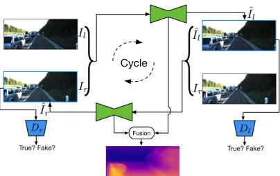
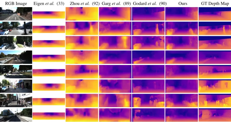
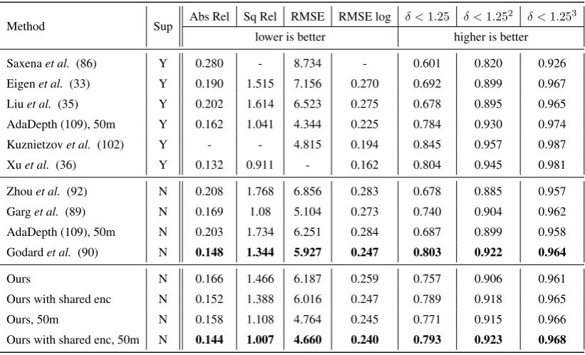
• An unsupervised depth estimation system (3) (Section 2.4) that makes use of a novel, cyclic and generative network architecture for stereo depth estimation.

Chapter 3 contains our work on few-shot learning, offering differing diversification strate-gies for generative systems:

• A few-shot classification system (4) (Section 3.2) that predicts a categorical 3D shape and predicted 3D meshes and textures for novel samples to diversify sample generation. The most representative generated samples are then selected through a self-paced learning module.

• Section 3.2 presents a second few-shot learning system that makes use of abundant tex-tual information to generate cross-modal features. A strategy to combine real and gener-ated features is suggested, allowing easy inference using only a simple nearest neighbour approach, the method outperforming competitors by a large margin.

Chapter 4 tackles issues arising in life-long learning systems when data storage is restricted, specifically catastrophic forgetting.

• A system to overcome catastrophic forgetting is presented, where we introduce a deep generative memory network that efficiently learns sparse attention maps, and dynami-cally expands its network capacity as new tasks arrive.

Finally, Chapter 5 holds the concluding remarks to the thesis, and prospective future works based on it.

1.1.5 Published Works

• "Unsupervised Tube Extraction Using Transductive Learning and Dense Trajectories" Mihai Marian Puscas, Enver Sangineto, Dubravko Culibrk, Nicu Sebe; The IEEE Inter-national Conference on Computer Vision (ICCV), 2015, pp. 1653-1661 (1)

• "Unsupervised Adversarial Depth Estimation using Cycled Generative Networks" An-drea Pilzer*, Dan Xu*, Mihai Puscas*, Elisa Ricci, Nicu Sebe; 2018 International Con-ference on 3D Vision (3DV)587-595 (3)

• "Low-Shot Learning from Imaginary 3D Model" Frederik Pahde, Mihai Marian Puscas, Jannik Wolff, Tassilo Klein, Nicu Sebe, Moin Nabi; WACV 2019 (4)

• "Learning to Remember what to Remember: A Synaptic Plasticity Driven Framework."; Oleksiy Ostapenko, Mihai Puscas, Tassilo Klein, Moin Nabi, NIPS CL Workshop 2018. (9)

• "Unsupervised Monocular Depth Estimation using Structured Coupled Dual Generative Adversary Networks"; Mihai Marian Puscas, Dan Xu, Andrea Pilzer, Nicu Sebe, Under review, IJCAI 2019

• "Adversarially Learned Feature Generating Network for Low-Shot Learning"; Frederik Pahde, Mihai Marian Puscas, Jannik Wolff, Tassilo Klein, Nicu Sebe, Moin Nabi, Under review, ICCV 2019

• "Learning to Remember: A Synaptic Plasticity Driven Framework for Continual Learn-ing"; Oleksiy Ostapenko, Mihai Puscas, Tassilo Klein, Moin Nabi, CVPR 2019 (5)

Unsupervised proposal systems

In this chapter we explore solutions developed to tackle an annotation scarcity for video and image understanding tasks. Section 2.2 presents a spatio-temporal localization system that extends a locally defined "objectness" proprety to the temporal domain using long term trajec-tories to create tubes around objects of interest, which are further extended in a transductive manner. The graph-based method expanded upon in section 2.3 provides an unsupervised pixel-level spatio-temporal segmentation. The segmentation and cutting graphs are jointly optimized, and different cues are organized into specific topologies that are automatically calibrated. Fi-nally, Section 2.4 provides a cycled, generative solution for stereo depth that does not require expensive LIDAR depth map annotations during the learning process.

2.1

Background

the broader application of these methods. In the case of spatio-temporal action detection sys-tems, or tasks which require this localization, the qualitative data scarcity can be ameliorated if there exists a system that outputs spatio-temporal proposals in an unsupervised manner, thus greatly simplifying an annotator’s workload.

InSection 2.2we detail an unsupervised, class agnostic spatio-temporal tube proposal sys-tem that outputs tubes covering objects of interest in a given video. This interest is determined through the use of motion cues, i.e. objects the are moving throughout the video are more likely to be of interest in further tasks, and annotating them will be beneficial. As all learning performed in the proposed method is transductive, it is class agnostic and can mine proposals on a broad range of videos.

The proposals are created by extending the local, image-level, ’objectness’ property to the temporal domain. ’Objectness’ can be defined as the likelyhood of an image window to contain an object instead of uninformative background (19, 20, 21, 22). Further, the goal of the work is to lighten a prospective annotator’s workload, leading to the need for highprecisionon the tube proposals in contrast to local, image-level object proposal systems that tend towards a high recall (19). This precision is achieved through a strict pruning of the intermediate tube proposals, followed by an appearance detection step that further filters out noise.

A limitation of the proposed system is a lack of temporal resolution, a consequence of the last stage of tube construction, where intermediate tubes are filtered and expanded using a transductive learning approach. This leads to a very poor temporal localization and limits its applicability to temporally constrained videos. A second limitation is a consequence of the temporal cues used to construct the initial tubes - only objects that are moving are considered to be of interest, an assumption that may be false when applying it broadly.

from ones based on clustering (25, 26), to graph-based processing (24, 27, 28, 29) and track-ing (30, 31, 32).

For the described system, we have chosen to map video elements onto a graph on which su-perpixels/supervoxels are nodes and edges measure similarity between them. Segmenting such a structure is generally actived in two steps: learning a similarity between nodes, and cutting the graph into semantically significant structures. Learning the similarity requires usable and cues whose weights we automatically learn and which are organized into different topological structures to keep them comparable (local, across one frame, across two frames, long term). Finally, to achieve an optimal segmentation, the graph cut and similarity are jointly optimized. In comparison to the work presented in section 2.2, this system provides a more comprehensive segmentation of a given video - with the caveat that the user must provide the total number of segments for the joint optimization to be achievable, and that any annotator will not receive any cues towards what objects might be of interest or not.

While the systems detailed in sections 2.2 and 2.3 tackle the lack ofqualityin available data through providing annotations for common video understanding tasks, there are cases where low-level features used in more complex learning tasks are expensive or even impossible to learn. This can be caused by a number of factors, such as the need of specialized sensing equipment that can be difficult to acquire and operate, require strict operating conditions, or that is simply too bulky to use in day-to-day activities.

One such case is estimating depth maps, which see broad use in various image and video understanding tasks, from robotics and autonomous driving, to virtual reality and 3D recon-struction. Great progress has been seen over the last years, with supervised deep regression methods significantly improving the accuracy of estimated depth maps (33, 34, 35, 36). The ap-plication of these systems is restricted by the need for high quality depth maps for the learning process, usually provided through the use of a LIDAR sensor, and compounding the problem, the large amount of depth maps needed to learn a deep model.

2.2

Unsupervised Spatio-Temporal Tube Extraction

2.2.1 Introduction

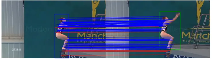
Figure 2.1: Optical Flow between two consecutive frames can be used as a ”voting” mechanism for matching Bonding Boxes. The blue lines are dense trajectories in common between the two

boxes, while the red lines are trajectory starting from the first box but not included in the second.

In this work we focus on extending the objectness property from still images to videos, to provide class agnostic spatio-temporal proposals for further video understanding tasks. Other works which deal with automatic tube proposals address this extension of objectness to the temporal domain. However, most of the state-of-the-art approaches have the same limitation: they need a lot of tubes (usually hundreds or thousands per video clip) to achieve a sufficiently high recall (10, 11) which makes these methods reliable to speed up the testing phase but not sufficiently precise to allow for weakly supervised or unsupervised training. Using two common benchmarks (UCF Sports and YouTube Objects) we will show that we are able to achieve high recall with few tubes. For instance, in UCF Sports we achieve more than 30% relative improvement with respect to the state-of-the-art when using only one tube (Fig. 2.4b). These results have been achieved by combining different ideas. First, we use Selective Search in order to produce an initial set of candidate BBs. Then we propose to use Dense Trajectories (37, 38) in order to match BBs in different frames and to discard static BBs. This method allows us to collect initial tubes that we calloptical flow tubesas they are based on the optical flow computed with Dense Trajectories. In order to avoid drifting (a common problem in all tracking algorithms), optical flow tubes are usually quite short and do not cover the

1

whole video clip. For this reason we propose using the optical flow tubes in order to collect positive samples of the moving objects and train tube-specific detectors. We highlight that no class labels or other human-provided information is used for training. Conversely, tube-specific object detectors are learned in atransductiveframework, i.e., we do not need these detectors to generalize to other videos, except the same video in which they have been trained. In fact, once trained, we run the detectors on the input videos in order to extract the final tubes (detection tubes). Using this strategy, we are able to extract BBs even in frames in which the object is static, while common tube-proposal approaches usually need movement in all the frames. To summarize, our contributions are:

• We use Dense Trajectories to robustly match BBs pre-selected by means of Selective Search.

• We use tube-specific,class agnosticdetectors, trained in a transductive learning frame-work, to extract the final tubes.

The code for the proposed approach is available2.

The rest of the chapter is organized as follows. In Sec. 2.2.2 we briefly review the literature and in Sec. 2.2.3 we introduce some useful notation which will be used in the other sections. In Sec.s 2.2.4 and 2.2.5 we present our method. Experimental results are shown in Sec. 2.2.6 and we conclude in Sec. 2.2.7.

2.2.2 Related Work

In (39), Prest et al. extract tubes from a video clip exploiting homogeneous clusters of dense point tracks. The tubes are then used to learn a detector, together with video-level-based labels and based on the assumption that there is one dominant moving object per video. It is worth noticing that, in the approach we propose, the detectors are class-agnostic classifiers which are learned for every optical flow tube and thenused to extract the final tubes. Conversely, in (39) the detectors are class-specific object detectors (fusing the segmentation phase with the final, unsupervised object classification phase). One drawback of this approach is that tubes are selected using inter-tube similarity, which is a fragile assumption when more than one moving object is present in the video clip and/or when a single object has a high variability of appearance.

Clustering dense tracks, obtained with optical flow, is a strategy adopted by many other authors. For instance in (40) point tracks are clustered using an affinity matrix based on the maximum translational difference between two tracks. Even if encouraging results can be obtained with this technique, articulated motion makes it hard to group tracks belonging to non-homogeneously moving objects. Optical flow is also used in (41), where objects are segmented using motion boundaries and then refined using a dynamic appearance model of the RGB foreground pixels. In (42) and in (43) optical flow and other appearance and saliency cues are used to extract coherent segments corresponding to moving objects.

In (10) the Selective Search (19) criteria for merging pixels in superpixels are extended into the time domain to obtain supervoxels. Supervoxels are used also in (11) with a hierarchical graph-based algorithm and in (44), where, instead of using heuristics, merging is performed using a classifier. In (45) motion boundaries are used in order to generate an initial set of moving object proposals, which is then ranked using a Convolutional Neural Network (CNN), trained using ground truth object BBs. It is worth noticing that both (44) and (45) aresupervised

methods, in which there is an important learning phase based on manually provided examples of ground truth objects and it is not clear what is the cross-dataset generalization capabilities of these systems (when tested on datasets different from the ones used for training), while our approach iscompletely unsupervised. A similar limitation holds in (46, 47), where a CNN is trained in order to regress multiple boxes likely containing objects. The idea behind (46, 47) is that static objectness can be learned using ground truth BBs contained in large datasets (Pascal and ILSVRC 2012). However, a dataset bias does exist (48), since the cross-dataset experiments presented by the authors show a drastic drop of performance of the net when trained with Pascal and tested on ILSVRC 2012 and a minor drop vice-versa.

2.2.3 Static Objectness and Notation

Given a video withTframes, we apply Selective Search (19) to each frameFtin order to extract

the set of box candidatesBt={bt1, ...btn}(we drop the superscripttwhen not necessary), and

bt

i = (ymini, xmini, ymaxi, xmaxi).

Note that we rely on Selective Search to modelstatic objectness. In other words, we do not manage pixel-level information, and we leverage on Selective Search for the pixel merging task in a single image. In fact this method is widely adopted and it has been proven to have a highrecall: for instance, withn= 2000, the probability of an object to be highly overlapping with anybt

using movement information in order to end up with a much smaller subset of boxes containing the moving objects of the video.

For simplicity, we also do not explicitly model the dynamics of the tracked boxes (which is difficult especially with ”random” movements of biological ”objects”). However, we use Intersection-over-Union (IoU) and Intersection-over-Min (IoM) in order to check spatial co-herence between boxes of different frames and in the same frame:

IoU(b1, b2) =A(b1∩b2)/A(b1∪b2), (2.1)

IoM(b1, b2) =A(b1∩b2)/min{A(b1), A(b2)}, (2.2)

where A(b) is the area of b. Both IoU and IoM are widely adopted metrics in the object detection literature (49, 50, 51, 52) to assess spatial coherence (IoU) and/or to merge small BBs in a larger rectangle (e.g., see the Non-Maxima-Suppression algorithm, NMS, used in (49, 52) and based on IoM).

Finally, we use Dense Trajectories (38) to extract dense trajectories of moving points. In (38) the authors use optical flow in order to track points over different frames. They also im-prove over (37) by estimating the camera motion and deleting those trajectories whose move-ment is similar to the camera motion. The final trajectories cluster over the actual moving objects most of the times (but unfortunately camera motion compensation is not able to delete all the noisy trajectories in the background). Trajectories are continuously created and termi-nated over the video frames and are usually very short (max 15 frames (37)), thus there are no trajectories spanning the whole video. Given two consecutive framesFtandFt+1, we define

the (camera motion compensated) optical flow betweenFtandFt+1as:

O(t, t+ 1) ={o1, ..., om}, (2.3)

whereoj = (pj, qj) is a local translational offset belonging to one of the active trajectories

between framesFtandFt+1,pj is the starting point (pj ∈ Ft) andqj the ending point (qj ∈

Ft+1).

2.2.4 Optical Flow Tubes

The first step of our pipeline consists in matching boxes inFtwith boxes inFt+1using optical

flow information and spatial coherence. GivenBtandBt+1, for eachbi ∈ Btandbj ∈ Bt+1

we define:

OV(i, j) :=IoU(bi, bj)≥0.5, (2.4)

where the threshold 0.5 is commonly adopted in object detection (e.g., in the Pascal and Ima-geNet detection tasks) to assess the spatial similarity of two BBs. Even if here the context is completely different (we useOV to prune BBs too far apart from each other in two different frames), we adopt the same threshold because it somehow guarantees that bi andbj can be

matched only when the difference in scale and/or aspect ratio is not that large. This constrains a (possibly articulated) movement of the object betweenFtandFt+1to produce a small

trans-lational difference and a moderate deformation. Ifn1 =|Bt|andn2 =|Bt+1|, thenOV is an

n1×n2Boolean matrix.

For eachbi, bj such thatOV(i, j) = true, we compute the optical flow-based matching

density betweenbiandbj, defined as:

D(i, j) := mij

A(bi) +A(bj)

, (2.5)

wheremij is the number of optical flow offsets inO(t, t+ 1)whose starting point is inbiand

ending point inbj. The intuitive idea behind Eq. (2.5) is straightforward. The nominator

repre-sents the number of "votes" that can be accumulated in matchingbiandbj, being each vote an

element inO(t, t+ 1). The denominator normalizes this number by the sum of the areas of the two BBs. This normalization is necessary because of noisy trajectories (e.g. trajectories laying on the background, despite camera motion compensation). In fact, maximizingmij without

area normalization leads to matchingbiwith thatbj inBt+1which is thelargestpossible, i.e.,

not a BB tight on the moving object but a BB usually including undesired background (e.g., see Fig. 2.1).

Using Eq. 2.5 we matchbiwithb∗j (and we writeMt(bi) =b∗j) such that:

b∗_j = max

bj∈Bt+1

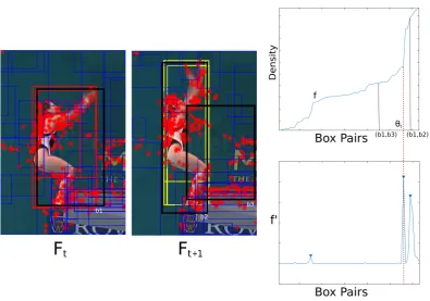
Figure 2.2: Adaptive threshold in matching density. Two consecutive frames with their initial

set of BBs. Both optical flow and BBs cluster around the moving object (left). In turn, clusters

correspond to plateaus inf, the sorted distribution ofD(right-top). The smoothed gradient offis used in order to detect peaks and to set the density threshold (right-bottom).

subject to:

D(i, j)_≥θt. (2.7)

In Eq. (2.7)θtis a threshold which is used to reduce the risk of drifting in tracking a BB.

Instead of using a fixed threshold, which is difficult to set, we adaptively computeθtfor every

pair of framesFtandFt+1, based on the observation that BBs produced by Selective Search

usually cluster around true objects and dense trajectories tend to cluster around moving objects due to the camera motion compensation process. Looking at Fig. 2.2 (left), BBsb1andb2, lying

on the moving object, also belong to two corresponding clusters of BBs, respectively in frame

Ft andFt+1 (depicted with red and yellow). The density value of those BB pairs belonging

Conversely, matchingb1 with a background BBb3, the corresponding density value is usually

drastically different. In Fig. 2.2 (right-top) we plot the value ofD, where the x-axis represents pairs of BBs sorted in ascending order with respect toD. Letf()be the sorted distribution of

D. Plateaus inf()correspond to pairs of BBs belonging to clusters inFtandFt+1, and these

clusters usually correspond to moving objects detected by Selective Search. We exploit this observation selectingθtas one of the steepest slopes inf. In Fig. 2.2 (right-bottom) we show

the (smoothed) gradient off, where peaks correspond to high variations inf before a plateau. We setθtto be the value offcorresponding to the median peak. Preliminary experiments with

θtequal to the last peak (higher density) gave slightly lower results.

Using Eq.s (2.4)-(2.7) we can compute single frame matchings Mt() for all the BBs in

Bt, whereMt(bi) is not defined (Mt(bi) = ∅) when there is nobj ∈ Bt+1 such that(bi, bj)

satisfies both constraints in Eq.s (2.4) and (2.7). We can then concatenate BBs in different frames forming a set ofchains CH = _{ch1, ch2, ...}, where a chainchis computed starting

from a given BBb0in framet(bo∈Bt) and:

ch= (b0, b1, ..., bi, bi+1, ..., bnc), (2.8) where:

bi+1=Mt+i(bi), (2.9)

Mt+nc(bnc) =∅. (2.10)

Chains are, on average, quite short (E(nc) ≈ 6in our experiments). For this reason we

further merge chains in optical flow tubes. We deal with the elements inCH as nodes in a graph, where an edge between two chainsch1, ch2 ∈CH is added when there is at least one

frame in common between ch1 andch2 such that the corresponding BBs in the two chains,

b1 ∈ ch1 andb2 ∈ ch2, satisfy: IoM(b1, b2) ≥ 0.5. Using IoM for measuring overlapping

(instead of IoU) has the advantage that small BBs lying on subparts of the object of interest are clustered (e.g., (49, 52)) Hence, connected components of this graph correspond to chains with a sufficient spatial overlap in at least one frame. We compute an optical flow tube (ot) for each of these connected components:

where eachri ∈ otis obtained by simply averaging the coordinates of those BBs b1, b2, ...

corresponding to the same frameFt (i.e., b1, b2, ... ∈ Bt) and respectively belonging to the

merged chainsch1, ch2, ...(i.e.,b1∈ch1,b2∈ch2, etc. ...).

The final optical flow tubes are relatively accurate. Still they only rely on two elements: the initial set of BBs provided by Selective Search and the matching pipeline described in this section, which is purely based on optical flow information. What is missing is a statistical model of the appearance of the tracked BBs, which can improve the result. We show in the next section how this model is computed.

2.2.5 Transductive learning

LetOT ={ot1, ot2, ...}be the set of optical flow tubes computed as described in the previous

section. For everyot∈OT we build a specialized classifier. We extract positive samples from the BBs inotand negative samples from other BBs in the video frames in whichotis defined and we train a linear SVM. The classifier obtained is then run on the whole video to obtain a new tube, that we call adetection tube.

This is a special case oftransductive learning, since the training samples are extracted, in anunsupervisedmanner, from the same video in which the classifier is tested. In other words, the aim of each classifier is to model the appearance of a tube and then use this model to refine the tube. We do not need that the classifier is able to generalize to other videos because it is only used for our tube extraction task.

The idea we propose is similar totracking by detectionapproaches, and it is exploited, for instance, in (53). The main difference of our approach with respect to (53) and other tracking by detection approaches is that our method is completely unsupervised, while in (53) a few positive BBs on the initial video frames need to be provided.

In more detail, given an optical flow tubeot = (r0, r1, ..., rno), we include all of its BBs in the positive set P. Moreover, if(Ft0, ..., Ftno) is the sequence of frames in which otis defined, we also include inPall those BBs which sufficiently overlap with one of the rectangles

r _∈ otin one of these frames, using the IoU criterion in Eq. (2.4). The negative set starts with an initial setN0 which is built including BBsbrandomly extracted in the first frameFt0

and such thatIoU(b, r0) ≤ 0.3. The threshold0.3 is widely adopted in the object detection

mining approach proposed in (50). Specifically, in a given frameFt∈(Ft0, ..., Ftno), givenP (which never changes) andNt, we train a classifierct= [wt, at]by minimizing:

wt, at= arg min

w,a

X

r∈P

max(0,1₋wφ(r)₋a) + (2.12)

X

r∈Nt

max(0,1 +wφ(r) +a) +λ||w||2 2,

whereφ(r) is a feature representing the BBr. Different kinds of features can be used. For instance, HOG features are quite fast to be extracted from a rectangular patch of an image. In our experiments we used CNN features:φ(r)is the 4096-dimensional feature vector extracted from the last fully-connected layer (F C7) of the ImageNet trained net described in (54). Note

that we donot perform fine tuning of the net’s parameters. In principle we could use all the sets of positivesP, extracted using all the optical flow tubes, in order to fine-tune the network before extracting our features. However, since the number of these tubes is small (on average, about 3 per video) and they are short, fine-tuning a network with millions of parameters (54) would probably lead to overfitting phenomena. Hence, we just use the net as a feature extractor, relying on the widely proven high discriminative skills of these features (55). Following (51) we also add some padding around eachr to include context. Finally, the value ofλ, which controls the influence of the regularization term, is chosen according to (51):λ= 10−4_{and the}

feature values are normalized as suggested in (51). Following a consolidated object detection pipeline and adopting the parameters suggested in (50, 51) allows us to avoid the necessity of tuning the parameters of our classifiers. We believe that this is of primary importance for the success of an unsupervised method because it does not force one to collect data to tune the parameters when the method is applied to a new domain.

Once trained,ctis tested on the BBs of the subsequent frames in whichotis defined, new

hard negatives are added and training is repeated (Eq. (2.12)). We refer to (50) for details on the hard negative mining procedure. The final classifier is given by the parameters computed in the last frame of the tube:c=ctno.

2.2.5.1 Detection Tubes

Once collected a set of classifiers C = {c1_{, ...,c}k_{}from a given video, the final part of our}

Figure 2.3:Flow chart of the proposed approach.

and a classifierci _{= [w}i_{, a}i_{]∈C, the highest scoring detection BBd}i

tofci inFtis obtained

maximizing:

di_t= arg max

b∈Bt

wiφ(b) +ai. (2.13)

Note that we use all the BBs inBtwhen ”testing” the classifier. We then build a detection

tubedti for each classifiercilinkingditover all theT frames of the video:

dti= (di1, ..., dit, ...diT). (2.14)

In this way we collect a setkdetection tubes, one per classifier. Note that the cardinality ofC,k, isnotfixed a priori, and it depends on the number of optical flow tubes constructed in the previous phase (see Sec. 2.2.4). In our experiments,kis usually very small (E(k)_≈3).

When many tubes are desired (e.g., to increase recall), we repeat training. More specifi-cally, wesplit a detection tubedt indt1_{, dt}2 _{using the criteria of the first stage (Sec. 2.2.4).}

Given two consecutive detections dt and dt+1 in dt, we split dt in dt1 = (d1, ..., dt) and

dt2 _{= (d}

t+1, ..., dT) when: IoU(dt, dt+1) < 0.5 orD(dt, dt+1) ≥ θt, where, with a slight

abuse of notation, D(dt, dt+1) is the match density defined in Eq. (2.5) and θt the adaptive

threshold pre-computed in the optical flow tube construction phase. After splitting the optical flow tubes, we use each tube to train a second set of classifiersC0 _{repeating the procedure} described in Sec. 2.2.5.

The final set of tubes for a given video is the set of the detection tubes obtained using all the detectors inC andC0. For a given videov, let DTv = {dt1, dt2, ...}be the set of all the

detection tubes obtained using all the classifiers inCandC0. In Fig 2.3 we show the flow chart of the whole procedure.

2.2.6 Experiments

2.2.6.1 Experimental Setup

DatasetsWe use for evaluation the UCF Sports dataset (56) and the YouTube Objects dataset (39). UCF Sports is composed of 150 videos of 10 sports (e.g., diving, running, golf, kicking, etc.). For evaluation we used the ground truth annotation provided in (44). Moreover, in order to allow a comparison with the results reported in (44), we adopted the same train/test split proposed in that article, where 100 videos are used for testing2. Note that in (44) the train split is used to train the proposedsupervisedmethod, while in ourunsupervisedapproach we only used this ”train” subset of 50 videos in the development stage to do all our design choices. We also do not have dataset-dependent parameters which need to be set (since all our parameter values are set using a consolidated object detection pipeline, see Sec.s 2.2.4-2.2.5), thus there is no training or parameter tuning phase in our approach, which makes the comparison with other supervised methods such as (44) disadvantageous for us since we do not exploit any dataset-specific information.

YouTube Objects is a large dataset composed of 1400 short shots obtained from videos col-lected on YouTube. As in the case of UCF Sports, many videos have large camera movement, illumination changes and cluttered backgrounds. However, the moving objects in this dataset usually occupy a larger portion of the frame, thus they are easier to detect. Differently from UCF Sports, in YouTube Objects there is only one annotated frame per shot but some frames are annotated with multiple objects. The dataset is split in a ”train’ and a ”test” subset. We used the ”test” shots to test our system (346 shots). Note that the ”train” shots are usually easier, thus testing on the whole dataset would probably get higher accuracy results.

MetricsFollowing (44) we use two metrics: mBAO and CorLoc. Both metrics are based on the Best Average Overlap (BAO) of a set of tube proposals with ground truth objects. In UCF Sports dataset there is only one moving object annotated per video (but the dataset contains some videos with more than one moving object, being only the predominant object provided of ground truth annotations). Using this assumption, for a given videovand a setDTv of tube

proposals forv, BAO is defined as follows (44):

BAO(v) = max

dt∈DTv 1

|Tv|

X

t∈Tv

IoU(dt, gt), (2.15)

2

The train/test split of the dataset and the annotations are provided at:

where|Tv|is the set of frames of videov with ground truth annotation,dtis the BB in tube

proposal dt at frame t, and gt is the ground truth at frame t. Note that in case of multiple

annotated objects per video (YouTube Objects dataset), Eq. (2.15) is applied separately to each object using the same set of proposalsTv (44). mBAO is the mean BAO across all the videos,

while CorLoc is the fraction of videos for which the BAO is greater or equal to 0.5.

2.2.6.2 Comparison with State of the Art

Number of tubes

1 10 100 1000

MBAO 0 10 20 30 40 50 60 70 Our method STODP [15] GBH [11] GBH-flow [11]

(a)mBAO computed over

the UCF Sport dataset.

Number of tubes

1 10 100 1000

50% CorLoc 0 10 20 30 40 50 60 70 80 Our method STODP [15] GBH [11] GBH-flow [11]

(b)CorLoc computed over the UCF Sport dataset.

Number of tubes

1 10 100 1000

50% CorLoc 10 20 30 40 50 60 70 80 90 100 Our method STODP-level 19 [15] STODP-level 15 [15] Prest [17] Papazoglou [16] Best from [3]

(c)CorLoc computed over the YouTube Objects dataset.

Figure 2.4:Quantitative results on UCF Sports and Youtube datasets

UCF Sports. In Fig.s 2.4a-2.4b we show the experimental results obtained on the ”test” part of UCF Sports dataset (100 videos). The methods we compare to are: (1) the Spatio-Temporal Object Detection Proposals (STODP) proposed in (44), (2) The Graph-Based Hier-archical segmentation proposed in (11) and its variant (2) GBH-Flow presented in (44). All the plotted results, except ours, have been obtained from (44).

YouTube Objects.Fig. 2.4c shows the results obtained with the YouTube Objects dataset. In this case we compare with two different parameter settings of STODP (we refer the reader to (44) for details), the unsupervised method proposed by Papazoglou et al. (41), the weakly supervised method of Prest et al. (39) and the result for the best tube among the proposals of the unsupervised method proposed by Brox and Malik (40). All the plotted results, except ours, have been obtained from (44) (mBAO is not provided by the other authors).

As Fig. 2.4c clearly shows, we outperform all the competitors, both the supervised and the unsupervised methods. The only approach which achieves a CorLoc value better than our system is (41), which only outputs a single proposal per shot. However, we obtain a CorLoc higher than (41) with only 4 proposals. Compared with Oneata et al. (44), which obtained 0.461when using 10 proposals, with the same number of tubes we obtain a CorLoc of0.596, a relative improvement of29%. Our largest value of CorLoc on this dataset is 0.927, obtained with 258 tubes, a recall much higher than any other published result.

2.2.6.3 Qualitative Results

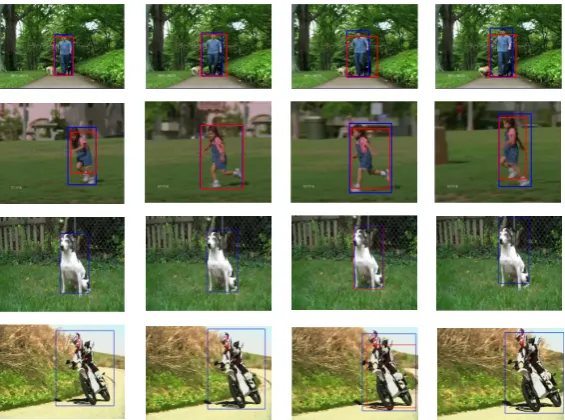
Figure 2.5:Some examples of detection tubes. In each row we show a tube taken from a different

video. 1-st and 2-nd row: UCF Sports dataset, 3-rd and 4-th row: YouTube Objects dataset. Red rectangles are BBs of the tube, while blue rectangles are ground truth annotations. Note that in

YouTube Objects, only one frame is provided with ground truth (3-rd column).

Figure 2.6: Some examples of errors of the proposed method. 1-st and 2-nd row: UCF Sports

dataset, 3-rd row: YouTube Objects dataset.

Youtube Objects images. Most of the times our system is able to accurately detect the moving object even when it stops for a while (e.g., the dog, which is still with respect to the background, despite there is camera movement), unlike most of the state-of-the-art methods which require movement in all the frames.

In Fig. 2.6 we show some incorrectly detected tubes. In the middle row the misalignment between the ground truth and the detections is probably due to the difference in speed of the upper part and the lower part of the person, which produced detectors only for the fastest part (the upper body). In the first row our system is actually able to accurately track most of the moving persons but, unfortunately, the UCF Sport dataset contains annotation for only one object (person) per video, penalizing the extraction of multiple-objects.

2.2.7 Conclusions

As a first step, we proposed a method for the extraction of tubes from videos based on a first pipeline in which optical flow obtained with Dense Trajectories is used for matching BBs and a second pipeline in which the initial tubes are used to collect positive training samples for training tube-specific detectors. The final tubes are given by the detections of the trained classifiers, used in a transductive framework. The method was evaluated on UCF Sports and YouTube Objects, showing state-of-the-art results.

2.3

Unsupervised Video Segmentation

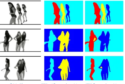
Video segmentation can be defined as partitioning a video into several disjoint spatio-temporal regions such that each region has consistent appearance and motion. In contrast to the method addressed in Section 2.2, the commonly accepted definition and benchmarks for this task as-sume that the segmentation is performed on a pixel level, with the high spatio-temporal seg-mentation accuracy that it implies. A high performance pixel-level spatio-temporal system mitigates the issues presented in the previous section.

2.3.1 Introduction

Among the existing video segmentation techniques, many successful ones benefit from map-ping the video elements onto a graph which pixels/superpixels are nodes and edge weights measure the similarity between nodes. Cutting or merging is then applied on this graph to generate the video segments. Most of the existing graph-based methods focus on (i) what fea-tures to extract from each node; (ii) how to define a precise similarity graph and (iii) how to cut/merge the nodes effectively.

Meaningful features are necessary for good video segmentation. Previous work has ex-tracted a variety of features (23, 26) from superpixels. To get the similarity graph, a graph topology is firstly designed according to the spatio-temporal neighborhood of the superpixels and the extracted features are used to weigh their edges. While standard similarity measures on the extracted features provide the basic way to calculate the similarity graph (25, 26), more recent work introduces learning a more precise similarity graph in either a supervised (27) or an unsupervised manner (57). While supervised video segmentation methods (23, 27) can gen-erally achieve better performance, the human annotation is time-consuming and the inherent video object hierarchy may be highly subjective. In contrast, a group of methods improve on cutting techniques (24, 25, 28, 29), which explicitly organize the image elements into math-ematically sound structures based on the optimization of the predefined cutting loss function. One representative criterion is the normalized cut (24). By minimizing a cutting cost objective function, the best segmentation can be obtained. This objective function is further proved to be equivalent to the generalized eigenvalue decomposition problem and a number of follow-ups

2

proposed efficient solutions for this problem (58). To reduce the computational cost, in (28, 29), fast partitioning methods that identify and remove between-cluster edges to form node clusters are proposed.

Graph cut methods provide well-defined relationships between the segments, but the prob-lem of finding a cut in an arbitrary graph may be NP-hard. More importantly, because the graph similarity learning (59, 60, 61, 62, 63, 64) and the graph cutting are conducted in two separated steps, the learned graph similarity matrix may not be the optimal one for cutting, leading to suboptimal results. To tackle this problem, in this paper we propose a novel video segmen-tation framework: Joint Graph Learning and Video Segmentation(JGLVS), which learns the similarity graph and segmentations simultaneously. To summarize, the main contributions of this paper are:

• Our unsupervised video segmentation framework learns the similarity graph and cutting structure simultaneously to achieve the optimal segmentation results. We derive a novel and efficient algorithm to solve this challenging problem.

• We utilized multiple cues of the superpixels and the weights of different cues are auto-matically learned. Furthermore, we calibrate the similarity of different superpixels based on their topology structures to make them comparable.

• The proposed JGLVS achieves up to 11% improvement over the state-of-the-art baselines on the largest public dataset VSB100, which validates the effectiveness and efficiency of our approach.

The remainder of this work is organized as follows. Section 2.3.2 discusses some related works. The details of JGLVS are introduced in section 2.3.3. Section 2.3.5 illustrates the experiments results and we draw a conclusion in section 2.3.6.

2.3.2 Related Work

The relevant state-of-the-art methods on video segmentation are reviewed in this section. The problem definitions for video segmentation have been diverse.

using group invariants. The actual grouping in these methods is done using spectral clustering. Differently, in (66), they formulate the segmentation of a video sequence based on point tra-jectories as a minimum cost multicut problem. Unlike the commonly used spectral clustering formulation, the minimum cost multicut formulation gives natural rise to optimize not only for a cluster assignment but also for the number of clusters while allowing for varying cluster sizes. Similarly, in (71), they utilize improved point trajectories to segment moving object in video by a graph-based segmentation method. And in (72), motion trajectory grouping in a setup similar to (68) is used to perform tracking. Although the grouping in (72) is computed using spectral clustering, repulsive weights computed from segmentation topology are used in the affinity matrix. In (65), they introduced minimal supervision, which is shown to be helpful to improve the performance of motion segmentations. In (73), they propose a framework to segment the objects in relative video shots, while discarding the irrelative video shots.

On the other hand, (26, 28, 29, 57) seek to construct full pixelwise segmentation, where every pixel (not only the moving objects) is assigned one of several labels. They can generally be divided into unsupervised and supervised methods.

A large body of literature exists on unsupervised video segmentation, with methods that leverage appearance (24, 30, 31, 74), motion (30, 75), or multiple cues (26, 28, 29, 57). Unsu-pervised supervoxel generation (26, 76) has been widely accepted as a valuable preprocessing step for various techniques, such as graph-based methods (24, 26, 28, 29), hierarchical meth-ods (24, 74, 77) and streaming methmeth-ods (28, 57, 74). Graph-based methmeth-ods map the video elements onto a graph in which pixels/superpixels are nodes, and edge weights measure the similarity between them. Galassoet al. (26) proposed a frame-based superpixel segmentation approach (VSS) by extending the ultra-metric contour map (78) to combine with motion-cues and appearance-based affinities for obtaining better video segmentation performance. To deal with the high computational costs of spectral techniques, Galassoet al.(28) proposed a spectral graph reduction (SGR) method for video segmentation. They assumed that all pixels within a superpixel are connected by must-link constraints, and then reduced the original graph to a relative small graph such that a density-normalized-cut was preserved. Yuet al.(29) proposed an efficient and robust video segmentation framework based on parametric graph partitioning, resulting in a fast and almost parameter free method. On the other hand, hierarchical video segmentation provides a rich multi-scale decomposition of a given video. Grundmannet al.

constructing a “region graph” over the obtained segmentation. Iteratively repeating this process over multiple levels results in a a tree of spatio-temporal segmentations. In order to process long videos, Xuet al.(74) proposed a streaming hierarchical video segmentation framework by integrating a graph-based hierarchical segmentation method with a data streaming algo-rithm (SHGB). This method leveraged ideas from data streams and enforced a Markovian as-sumption on the video stream to approximate full video segmentation. Liet al.(57) proposed a Sub-Optimal Low-rank Decomposition (SOLD) method, which defines a low-rank model based on very generic assumption that the intra-class supervoxels are drawn from one identical low rank feature subspace, and all supervoxels in a period lie on a union of multiple subspaces, which can be justified by natural statistic and observations of videos. In addition, this method adopts the Normalized-Cut (NCut) algorithm with a solved low-rank representation to segment a video into several spatio-temporal regions. To tackle the lack of a common dataset with suf-ficient annotation and the lack of an evaluation metric, a united video segmentation benchmark was provided by Galassoet al. (79) to effectively evaluate the over- and under-segmentation performance of video segmentation methods.

Supervised video segmentations (27, 80) can achieve better performance, but the human annotation is time-consuming and the inherent video object hierarchy may be highly subjective. In (80), they address the problem of integrating object reasoning with supervoxel labeling in multiclass semantic video segmentation. They first propose an object augmented dense CRF in spatio-temporal domain, which captures long-range dependency between supervoxels, and imposes consistency between object and supervoxel labels. Then, they develop an efficient mean field inference algorithm to jointly infer the supervoxel labels, object activations and their occlusion relations for a moderate number of object hypotheses. While in (27), they propose to combine features by means of a classifier, use calibrated classifier outputs as edge weights and define the graph topology by edge selection. Learning the topology provides larger performance gains and benefits efficiency due to a sparser structure of the constructed graph. On the other hand, lots of supervised image segmentations have been proposed (81). In (82), they propose a novel discriminative deep feature learning framework based on stacked autoencoders (SAE) to tackle the problem of weakly supervised semantic segmentation. In (81), they use CNN to train images most only with image-level labels and very few with pixel-level labels for semantic segmentation.

Videos

Features/Distances

Video Segmations Superpixels generation

on temporal sliding windows

lab cbs

sti

JGLVS

Similarity Graph S with K components

Figure 2.7:The overview of JGLVS. Superpixels are firstly generated from the overlapping sliding

windows, based on which the features and distances are computed. Then, JGLVS is applied to learn the similarity matrix and video segmentations.

obtaining a graph and finding a cut in it, we propose a joint graph learning and video seg-mentation method by assigning adaptive neighbors for each superpixel and imposing a rank constraint on the Laplacian matrix of the similarity graph, such that the learned graph has exactly K connected components, representing K segmentations.

2.3.3 Our Approach

In this section, we first introduce our JGLVS framework, and then elaborate on the details of each component.

2.3.3.1 The framework

In our JGLVS framework (see Fig. 2.7), we propose a novel perspective in solving the graph-based video segmentation problem. Our model makes use of superpixels instead of pixels for two reasons: a great decrease in the number of graph nodes that need to be processed, and an initial, accurate frame-level segmentation.

Firstly, in each temporal sliding window of the video, we extract N superpixels from

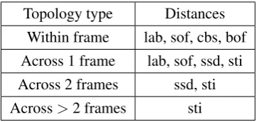
under-Topology type Distances Within frame lab, sof, cbs, bof Across 1 frame lab, sof, ssd, sti

Across 2 frames ssd, sti

Across>2 frames sti

Table 2.1:The corresponding distances for different topological structures

segmentation errors, while a large value ofN is computationally expensive. Then, for each superpixle, a set of features (e.g., appearance, motion and shape features) are extracted. Us-ing these features and the predefined topology structure, our JGLVS framework can learn a similarity graph of superpixels which has exactlyK connected components.

2.3.3.2 Feature extraction and graph topology construction

For each superpixel, we follow (26, 76) to extractLAB,boundary,motionandshapefeatures, and use them to calculate the distance between two superpixels. However, not all of the su-perpixels are connected. By allowing different edge connections between neighbors, different graph topologies are constructed. Following (24, 27), edges may connect neighbors: within frame(if two superpixels share a common part of their contour or are close by in the spatial domain of the frame);across 1 frame(connected by coordinate correspondences over time);

across 2 frames (connected by across-1 correspondences, further propagated over one more frame) andacross>2 frames(linked if overlapping with common long-term point trajecto-ries).

We refer to these four types of neighbours as different topological structures(1,2,3,4)and record the topological structure of each pair of superpixels in aN _×N matrixW. Based on these features and topological structures, we can have the following pairwise distances between superpixels: common boundary strength (cbs), LAB (lab), boundary optical flow (bof), super-pixel optical flow (sof), superpixel shape distance (ssd) and superpixel trajectory intersection (sti) (See Section 2.3.5 for details).

merge into one superpixel. These similar superpixels will be selected as the within frame most-likely-linked superpixels. For the case of across 1 or 2 frame, if two superpixels’ssddistance is less than a threshold, they will be selected as a pair of across 1 or 2 frame most-likely-linked su-perpixels. Similarly, if two superpixels’stidistance is less than a threshold in the case of across

>2 frame, they will be selected as a pair of across>2 frame most-likely-linked superpixels.

2.3.3.3 Joint graph learning and video segmentation

Let Dt = _{Dt_ij}N_i,j=1 denote the t-th distance matrix of a set of N superpixels, wheret _∈

{1, ..., T_}.Y=_{y₁,y₂, ...,y_N}is the average location information for the superpixels. The goal is to learn the similarity matrixSbetween superpixels by using different distances as well as existent spatial information, and that all the superpixels have exactKconnected components.

An optimal graphSshould be smooth on different features as well as on the spatial infor-mation distribution, which can be formulated as:

min

S,α g(Y,S) +µ

XT

t=1α

t_{h D}t_,S

+βr(S, α) (2.16)

whereg(Y,S)is the penalty function that measures the smoothness ofSon the spatial infor-mationYandh Dt,S

is the loss function that measures the smoothness ofSon the feature

Dt. r(S,ff)is a regularizer defined on the targetSandα. µandβ are balancing parameters, andfft_{determines the importance of each feature.}

The penalty functiong(F,S)should be defined in a way such that close superpixels have high similarity and vice versa. In this paper, we define it as follows:

g(Y,S) =X

ij

y_i−y_j

2

2sij (2.17)

wherey_i andy_j are the locations of the superpixelsxi andxj. Similarly,h Dt,S

is defined as:

h Dt,S

=X

ijd t

ijsij (2.18)

The regularizer termr(S, α)is defined as:

r(S, α) =kSk2F +γkαk 2

2 (2.19)

constraints: S _≥ 0, S1 = 1, α ≥ 0andαT_{1 = 1, where1 is a column vector with all1s.}

This is because that the similarity and weights should be positive, and the sum of similarity and weights is set to be 1.

We can then obtain the objective function for learning the optimal graph by replacing

g(Y,S),h Dt,Sandr(S, α)in (2.16) using (2.17), (2.18) and (2.19), as follows: min

S,α

P

ij

y_i−y_j

2

2sij+µ

P

tij

αt_dt ijsij

+β_kS_k2_F +βγ_kα_k2₂

s.t., S≥0,S1=1, α≥0, αT_{1= 1}

(2.20)

One limitation for this model is that it assumes that all the superpixels have the same types of distances, which conflicts with the video segmentation application where different topolo-gies have different distances. For example, if superpixels (i,k) are across>2frames neighbors and (i,j) are within frame neighbors, the similarity between (i,k) are determined bystibut the similarity between (i,j) are determined bylab, sof, cbsandbof. Their distances are not compa-rable to each other, and we need to calibrate them. Based on the topology typewij ∈[1,2,3,4]

of superpixelsiandj, we define a calibration function

cz(x) = (x−τz)/(maxz−τz), z∈[1,2,3,4], (2.21) whereτz _{is the threshold forz-th topology type determined by the mean distance of the set}

Mz. Then, the objective function becomes:

min

S,α

P

ij k

yi−yjk2₂sij +µP ij

cwij

P

t

αt_dt ij

sij

+βkSk2F +βγkαk 2 2

s.t., S≥0,S1=1, α≥0, αT_{1= 1}

(2.22)

Forcing the number of connected components to be exactly K seems like an impossible goal since this kind of structured constraint on the similarities is fundamental but also very difficult to handle. In this paper, we will propose a novel but very simple method to achieve this goal.

The matrix S _∈ RN×N obtained in the neighbor assignment can be seen as a similarity matrix of the graph with theN data points as the nodes. For a nonnegative similarity matrix

S, there is a Laplacian matrixLassociated with it. According to the definition of Laplacian matrix, for any values offi ∈RK×1,Lof a similarity matrixScan be calculated as:

X

ijkfi−fjk 2

2sij = 2tr F T_LF

whereF _∈ RN×K with thei-th row formed by fi, L = D− S

T

+S

2 is called the Laplacian

matrix in graph theory, the degree matrixD_∈RN×N is defined as a diagonal matrix where the

i-th diagonal element isP

j(sji+sij)/2. The Laplacian matrixLhas the following property. Theorem 1 The numberKof the eigenvalue0of the Laplacian matrixLis equal to the number of connected components in the graph with the similarity matrixSifSis nonnegative.

Theorem 1 indicates that if rank(L) = N −K, then the superpixels haveK connected components based on S. Motivated by Theorem 1, we add an additional constraintrank(L) =

N₋Kinto the (2.22). Thus, our new similarity graph learning model is to solve: min

S,α

P

ij

y_i−y_j

2

2sij +µ

P

ij cwij

P

t

αt_dt ij

sij

+βkSk2F +βγkαk 2 2

s.t.

S_≥0,S1=1, α_≥0, αT_{1= 1}

rank(L) =N ₋K

(2.24)

It is difficult to solve the problem (2.24). BecauseL =D−(ST +S)/2andDalso depends onS, the constraintrank(L) = N ₋K is not easy to tackle. In the next subsection, we will propose a novel and efficient algorithm to solve this challenging problem.

2.3.4 Iterative optimization

Suppose ei is thei-th smallest eigenvalue of L, we know ei ≥ 0 sinceL is positive

semi-definite. It can be seen that the problem (2.24) is equivalent to the following problem for a large enough value ofρ:

min

S,α

P

ij

y_i−y_j

2

2sij +µ

P

ij cwij

P

t

αt_dt ij

sij

+β_kS_k2_F +βγ_kα_k2₂+ 2ρPK

i=1

ei

s.t., S≥0,S1=1, α≥0, αT_{1= 1}

(2.25)

Whenρis set to a large enough value2,PK

i eiwill be imposed to be close to0, which results

inrank(L) =N −K. 2

According to the Ky Fan’s Theorem (83), we have:

K

X

i=1

ei = min

F∈RN×K,FTF=I

tr FTLF

(2.26)

Therefore, the problem (2.25) is further equivalent to the following problem:

min

S,F,α

P

ij

y_i−y<