Testing Ostrom: an Analysis of Water User Committees in Uganda

(1)

The University of San Francisco

USF Scholarship: a digital repository @ Gleeson Library |

Geschke Center

Master's Theses Theses, Dissertations, Capstones and Projects

Summer 8-29-2014

Mechanistic Studies of Salt Effects on Bimolecular

Electron-Transfer Reactions of Pentaamine

Ruthenium Pyridyl Complexes Studied by 19F

NMR Line-Broadening and T2 Spin-Echo

Techniques

Nicholas J. Magarian

[email protected]

Follow this and additional works at:https://repository.usfca.edu/thes

Part of theInorganic Chemistry Commons, and thePhysical Chemistry Commons

This Thesis is brought to you for free and open access by the Theses, Dissertations, Capstones and Projects at USF Scholarship: a digital repository @ Gleeson Library | Geschke Center. It has been accepted for inclusion in Master's Theses by an authorized administrator of USF Scholarship: a digital repository @ Gleeson Library | Geschke Center. For more information, please [email protected].

Recommended Citation

Magarian, Nicholas J., "Mechanistic Studies of Salt Effects on Bimolecular Electron-Transfer Reactions of Pentaamine Ruthenium Pyridyl Complexes Studied by 19F NMR Line-Broadening and T2 Spin-Echo Techniques" (2014).Master's Theses. 101.

(2)

Mechanistic Studies of Salt Effects on Bimolecular Electron-Transfer

Reactions of Pentaamine Ruthenium Pyridyl Complexes Studied by

19

_{F NMR Line-Broadening and T}

2

Spin-Echo Techniques

A Thesis Presented to the Faculty of the Department of Chemistry at the University of San Francisco

in partial fulfillment of the requirements for the Degree of Master of Science in Chemistry

Written by

Nicholas Magarian

Bachelor of Science in Chemistry

California Polytechnic State University, San Luis Obispo, California

(3)

Mechanistic Studies of Salt Effects on Bimolecular Electron-Transfer

Reactions of Pentaamine Ruthenium Pyridyl Complexes Studied by

19

_{F NMR Line-Broadening and T}

2

Spin-Echo Techniques

Thesis Written By Nicholas Magarian

This thesis is written under the guidance of the Faculty Advisory Committee, and approved by all its members, has been accepted in partial fulfillment of the

requirements for the degree of

Master of Science in Chemistry

at

The University of San Francisco

Thesis Committee

Jeff Curtis, Ph. D. Research Advisor

Tami Spector, Ph. D. Professor

William Melaugh, Ph. D. Professor

(4)

Acknowledgements

I would first like to acknowledge my advisor Dr. Jeff Curtis for his patience,

support, and guidance, as well as for providing me with skills I will carry with me

throughout my career. I would like to give a special thanks to Dr. William Melaugh

and Dr. Tami Spector for their advice and time in reviewing my work. I would also

like to thank the technical support staff: Jeff Oda, Andy Huang, Chad Schwietert, and

Angela Qin for all their assistance throughout my time at USF. I would also like to

thank the program assistant, Deidre Shymanski, as well as the USF chemistry

department staff. Finally, to my family and friends, thank all of you for listening and

(5)

iv

Table of Contents

Chapter 1 - An Overview of Electron-Transfer Reactions

1.1 Introduction ...1

1.2 Complementary Aspects Between Thermal and Optical ET ...2

1.2.1 Thermal ET ...2

1.2.2 Optical ET ...5

1.3 The Outer-Sphere Mechanistic Pathway for Activated ET ...7

1.4 The Reorganizational Energy Barrier, λ, Associated with ET ...11

1.4.1 The “inner-sphere” reorganizational energy, λin ...13

1.4.2 The “outer-sphere” (solvent) reorganzational energy, λout ...14

1.5 Potential Energy Surfaces ...16

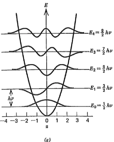
1.5.1 The harmonic oscillator approximation ...16

1.5.2 Potential energy surfaces in the “zero-order” diabatic limit ...21

1.5.3 Potential energy surfaces to first-order (adiabatic ET) ...24

1.5.4 The ET rate expression ...25

1.6 Quantum Super-Exchange Theory of HAB Modulation ...31

1.7 Debye-Hückel Theory and the Effects of Ionic Strength on Activity Coefficients ...34

(6)

v

Chapter 2 - Kinetic Studies of Salt Effects and Concentration Effects of

Reactants on Self-Exchange Reactions Monitored by 19F NMR Spectroscopy

2.1 Introduction ...61

2.1.1 Known effects of added simple salts on ET rates ...65

2.1.2 Known effects of added dicarboxylate salts on the rate of ET ...70

2.1.3 Known effects of added hexacyano complexes (K4M(CN)6,

where M= FeII, RuII, OsII) on the rate of ET ...75

2.2 Determination of Kinetic Rate Constants from NMR Line-Broadening

and T2 ...79

2.3 The T2 Spin-Echo Experiment ...90

2.4 Synthesis and Purification of Reactants and Salts ...98

2.4.1 Preparation of ruthenium(III)chloropentaaminedichloride,

[(NH3)5RuIIICl]Cl2...98

2.4.2 Recrystallization of ruthenium(III)chloropentaaminedichloride,

[(NH3)5RuIIICl]Cl2...99

2.4.3 Preparation of Zn/Hg amalgum ...99

2.4.4 Preparation of ruthenium(II)L-pentaamminehexafluorophosphate,

[(NH3)5RuII-L](PF6)2, where L= tfpm ...100

2.4.5 Acetone/Ether purification pentaammineruthenium(II)-L-

hexafluorophosphate, [(NH3)5RuII-L](PF6)2 where L= tfpm ...101

2.4.6 Preparation of pentaamineruthenium(II)-L-chloride,

[(NH3)5RuII-L]Cl2 where L = tfmp ...101

(7)

vi

2.4.7 Preparation of pentaamineruthenium(III)-L-chloride,

[(NH3)5RuIII-L]Cl3, where L = tfmp ...102

2.4.8 Preparation of disodium dicarboxylate salts, Na2-X, where X = muc, tere, 1,4-dcch, adip ...103

2.4.9 Preparation of potassium ruthenocyanide, K4RuII(CN)6 ...103

2.4.10 Preparation of potassium osminocyanide, K4OsII(CN)6 ...104

2.4.11 Recrystallization of potassium ferrocyanide, K4FeII(CN)6 ...104

2.4.12 Recrystallization of potassium hexacyano complexes, K4M(CN)6, where M = RuII, OsII ...105

2.5 Solution Preparation...106

2.5.1 Solution preparation of reactant solutions for NMR ET self-exchange measurements ...106

2.5.2 Solution preparation for added-salt NMR kinetic measurements ....107

2.6 NMR Instrument Set-Up and Experiment Execution ...108

2.6.1 Setting up the 19F NMR experiment ...108

2.6.2 NMR pulse calibration ...109

2.6.3 Setting up the 19F spin-lattice (longitudinal) relaxation, T1, experiment ...114

2.6.4 Setting up the 19F T2 spin-echo experiment ...120

2.6.5 NMR probe/sample temperature calibration ...124

2.7 Experimental Methodology used in Measuring Kinetic Salt Effects ...132

2.8 Sample Degassing ...133

(8)

vii

2.8.2 Degassing by vacuum ...134

2.8.3 Saturation with oxygen ...136

2.9 Methods for Assessing the Effects of Degassing on the 19F T2 Spin-Echo ET Kinetic Measured with added Sodium Muconate ...136

2.10 NMR Temperature Dependent Kinetic Experiments ...138

2.10.1 Line-broadening measurements ...138

2.10.2 19F T2 spin-echo measurements ...139

2.11 Validation of the 19F T2 Spin-Echo Experiment ...140

2.12 Reactant Concentration Effects on the Rate of ET (Self-Salting) ...146

2.13 Kinetic Salt Effects at Various (Constant) Reactant Concentrations ...151

2.14 Sodium Muconate Effects on the Rate of ET as Established by NMR ...173

2.15 Effect of Added Group VIII Metal Hexacyano Salts on the Rate of ET ...185

2.16 Temperature Dependent Kinetic Studies ...195

2.16.1 Reactant concentration effects on activation parameters ...198

2.16.2 The effects of added salts on activation parameters ...211

2.16.3 Effects of added Group VIIIb hexacyano salts on reaction (2-2) activationparameters ...231

2.17 Kinetic Modeling ...243

2.17.1 Application of our model to self-salting data ...254

2.17.2 Salt-specific kinetic modeling at 0.10 mM reactants ...259

(9)

viii

2.17.6 Kinetic modeling of added hexacyano’s at 0.10 mM reactants ...321

2.17.7 Kinetic modeling of added hexacyano’s at 5.00 mM reactants ...326

2.18 Discussion ...332

2.19 Conclusions ...347

(10)

ix

List of Figures

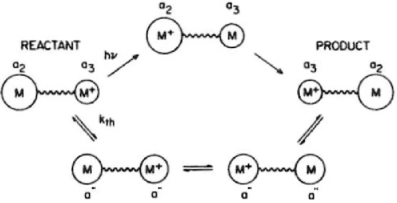
Figure 1.1 Optical and thermal ET mechanisms ...3

Figure 1.2 Harmonic osciallator and associated wavefunctions ...18

Figure 1.3 Potential energy surfaces showing non-adiabatic ET ...22

Figure 1.4 Potential energy surfaces showing adiabatic ET ...25

Figure 1.5 Surfaces and vibrational levels relevant to the three types of tunneling processes in the quantum non-adiabatic ET model ...30

Figure 1.6 The “electron-transfer” and “hole-transfer” quantum super-exchange mechanisms ...34

Figure 1.7 The collective charge-dipole behavior which results in the bulk observable Ds allowing for the medium to be treated as a “polarizable isotropic continuum” ...38

Figure 1.8 The first and second hydration spheres around the reactant ions forming the Debye-Hückel ion-atmosphere ...39

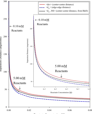
Figure 1.9 A simple cubic “lattice” model which can be used to calculate the effective center-center interreactant distance ...49

Figure 1.10 A representation of the interpenetrating crystal lattice structures ...51

(11)

x

Figure 2.1 A schematic of reaction (2-1), the “pseudo-self-exchange” reaction

between [(NH3)5RuII3-Fpy]2+ and [(NH3)5RuIIIpy]3+ ...61

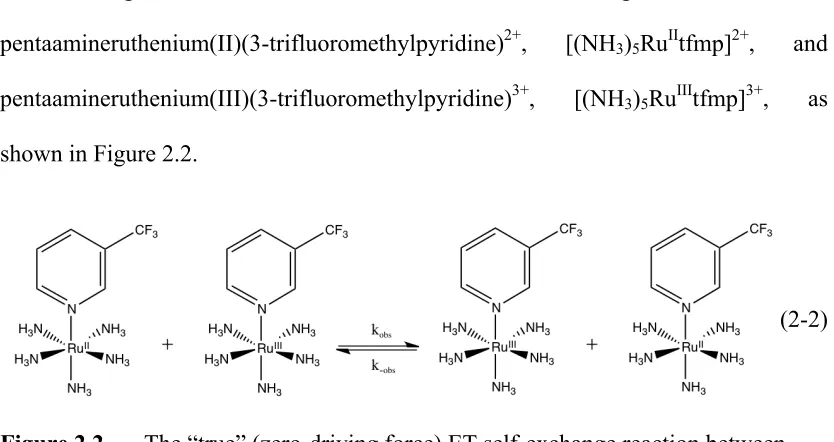
Figure 2.2 A schematic of reaction (2-2), the “true” (zero-driving force) ET

self-exchange reaction between [(NH3)5RuIItfmp]2+ and

[(NH3)5RuIIItfmp]3+ ...62

Figure 2.3 Effect of the halide salts on the rate of reaction (2-1) measured by

stopped-flow at an equimolar reactants concentration of 0.10 mM ...67

Figure 2.4 Effect of the halide salts on the rate of reaction (2-2) measured by

NMR line-broadening at an equimolar reactants concentration of

5.00 mM ...69

Figure 2.5 Effect of the dicarboxylate salts on the rate of reaction (2-1) measured

by stopped-flow at an equimolar reactants concentration of

0.10 mM ...72

Figure 2.6 Effect of the dicarboxylate salts on the rate of reaction (2-2) measured

by NMR line-broadening at an equimolar reactants concentration of

5.00 mM ...74

Figure 2.7 Effect of the hexacyano salts on the rate of reaction (2-1) measured

by stopped-flow at an equimolar reactants concentration of

(12)

xi

Figure 2.8 Effect of the hexacyano salts on the rate of reaction (2-2) measured

by NMR line-broadening at an equimolar reactants concentration of

5.00 mM ...78

Figure 2.9 A schematic illustration of how NMR peak resonances arise ...81

Figure 2.10 An illustration of how NMR line-shapes depend on exchange rate

processes as the magnitudes of  and T are varied ...87 ₂

Figure 2.11 The CPMG T2 spin-echo pulse sequence diagram ...94

Figure 2.12 The rotating frame depiction the net of magnetization vector and

Isochromat behaviors during execution of the T2 spin-echo pulse

sequence ...95

Figure 2.13 An illustration of a pw90 determination via peak intensity vs.

angular rotation plot out past pw360 ...111

Figure 2.14 A coarse pw90 calibration curve for the complex

[(NH3)5RuIItfmp]Cl2 in D2O at a concentration of 5.00 mM using

the 19F nucleus...113

Figure 2.15 A screenshot of the “Channels” sub-tab showing the correct

parameters for the 19F T1 inversion-recovery determination ...115

Figure 2.16 A screenshot of the “Acquisition” sub-tab showing the correct

parameters for the 19F T1 inversion-recovery determination ...116

Figure 2.17 A screenshot of the “Array Parameter” window for the 19F T1

inversion-recovery experiment on the [(NH3)5RuIItfmp]Cl2 complex

(13)

xii

Figure 2.18 The 19F T1 inversion-recovery pulse sequence displaying

parameters associated with the [(NH3)5RuIItfmp]Cl2 complex

in D2O at a concentration of 5.00 mM ...118

Figure 2.19 An example of the 19F T1 inversion-recovery curve corresponding to

the spin-lattice relaxation of the [(NH3)5RuIItfmp]Cl2 complex in D2O

at a concentration of 5.00 mM ...120

Figure 2.20 The 19F T2 spin-echo pulse sequence displaying the

parameters associated with the [(NH3)5RuIItfmp]Cl2 complex in D2O

at a concentration of 5.00 mM ...123

Figure 2.21 An example of The 19F T2 spin-echo decay curve of the

[(NH3)5RuIItfmp]Cl2 complex in D2O at a concentration of

5.00 mM ...124

Figure 2.22 The 1H NMR spectrum of the standard 100% methanol sample

displaying the chemical shift difference between the two peaks,

Δδ, arising from the -OH and -CH3 functional groups of

the methanol ...125

Figure 2.23 The temperature calibration curve obtained over the range of

263.15 K (-10°C) to 328.15 K (55°C) using the standard 100%

methanol sample ...128

Figure 2.24 The instrument readout temperature error as the increment

(TSample – TReadout) over the temperature range 263.15 K (-10°C) to

(14)

xiii

Figure 2.25 The measured logkexvs. GP behavior found for reaction (2-2) as

measured by the T2 spin-echo method and NMR line-broadening

data as well as for reaction (2-1) measured previously by

stopped-flow ...148

Figure 2.26 The effect of added KF, NaCl, and KBr on the measured kex for

reaction (2-2) at a reactants a concentration of 0.10 mM ...155

Figure 2.27 The effect of added Na2muc, Na2adip, Na2tere, Na2(1,4-dcch), KF,

and KBr on the kex for reaction (2-2) at a reactants concentration of

0.10 mM ...156

Figure 2.29 The effect of added Na2muc, Na2adip, KF, and KBr on the kex for

reaction (2-2) at a reactants concentration of 0.50 mM ...163

Figure 2.30 The effect of added KF, NaCl, KBr, and Na2muc on the measured kex

for reaction (2-2) at a reactants a concentration of 1.00 mM ...166

Figure 2.32 The effect of added Na2muc, Na2adip, KF, and KBr on the kex for

reaction (2-2) at a reactants concentration of 5.00 mM ...170

Figure 2.33 The effect of added Na2muc on the rate of ET for reaction (2-1) as

measured by stopped-flow6_{compared to the effect on the rate of}

reaction (2-2) found using the T2 spin-echo NMR method at the

(15)

xiv

Figure 2.34 The effect of sodium muconate on the rate of ET for reaction (2-2) as

measured by T2 at a reactants concentrations of 0.10 mM in D2O and

H2O ...178

Figure 2.35 Degassing and O2-saturation effects on the rate of reaction (2-2) in

D2O at a reactants concentration of 0.10 mM using raw logkex

values for the effects of air-saturation, vacuum degassing, Ar

degassing, and O2 saturation.. ...181

Figure 2.36 Degassing and O2-saturation effects on the rate of reaction (2-2) in

D2O at a reactants concentration of 0.10 mM using logkex values

normalized to the average logkex starting value for effects of air-

saturation, vacuum degassing, Ar degassing, and O2 saturation...182

Figure 2.37 The temporal decay of the measured logkex over a period of 25

minutes for reaction (2-2) at a reactants concentration of 5.00 mM

with the addition of K4FeII(CN)6 at 0.01 mM ...188

Figure 2.38 The stability of the measured logkex over a period of 25 minutes for

reaction (2-2) at a reactants concentration of 5.00 mM with the

addition of K4FeII(CN)6 at 0.39 mM ...189

Figure 2.39 The effect of added K4FeII(CN)6, K4OsII(CN)6, and K4RuII(CN)6 on

kex for reaction (2-2) at a reactants concentration of 5.00 mM along

(16)

xv

Figure 2.40 The effect of added K4FeII(CN)6, K4OsII(CN)6, and K4RuII(CN)6 on

kex for reaction (2-2) at a reactants concentration of 0.10 mM along

with previous results obtained via stopped-flow (reaction 2-1) by

Mehmood ...194

Figure 2.41 Erying plots of the data in Tables 2.21 and 2.22 at equimolar

reactants concentrations of 0.10 mM, 0.50 mM, 3.00 mM,

5.00 mM, 5.30 mM, 5.50 mM, 6.50 mM, and 8.00 mM ...204

Figure 2.42 The approximately linear relationship between ΔH≠vs. GP (reactant concentrations ranging from 0.10 mM to 8.00 mM) for reaction (2-2)

as taken from Table 2.24 ...207

Figure 2.43 The approximately linear relationship between ΔS≠vs. GP (reactant concentrations ranging from 0.10 mM to 8.00 mM) for reaction (2-2)

as taken from Table 2.24 ...208

Figure 2.44 ΔH≠vs.ΔS≠ for reaction (2-2) at reactant concentrations ranging from 0.10 mM to 8.00 mM showing evidence for enthalpy-entropy

compensation ...210

Figure 2.45 Temperature dependent normalized rate data for reaction (2-2) at

0.10 mM reactants with no added salt, added KF (1.80 mM), KBr

(1.80 mM), Na2muc (0.60 mM), and Na2adip (0.60 mM) ...214

Figure 2.46 Temperature dependent rate data for reactions (2-1) and (2-2)

observed via stopped-flow and T2 spin-echo, respectively, at

0.10 mM reactants with added KF (1.80 mM), Na2muc (0.60 mM),

(17)

xvi

Figure 2.47 Enthalpy-Entropy compensation at a 0.10 mM reactants in the

presence of KF, KBr, Na2Muc, and Na2Adip ( non-forcing

conditions, GP = 0.0494) for reaction (2-2) studied by NMR

compared with the entire halide series and dicarboxylate salts for

reaction (2-1) studied by stopped-flow ...220

Figure 2.48 Temperature dependent normalized rate data for reaction (2-2) at

0.10 mM reactants with no added salt (GP=0.0291), added KF

(6.00 mM), and KBr (6.00 mM) such that the total solution GP

was 0.0767 (“forcing conditions”) ...223

Figure 2.49 Enthalpy-Entropy compensation at 0.10 mM reactants in the

presence of KF and KBr (forcing conditions, [X-] = 0.006 M) for

reaction (2-2) studied by NMR compared with kinetic data for the

entire halide series obtained in studies of reaction (2-1) by

stopped-flow ...228

presence of the halides and dicarboxylate salts for reaction (2-2)

studied by NMR (red circles) compared with kinetic data for the

entire halide series and dicarboyxlate salts obtained in studies of

reaction (2-1) by stopped-flow6 (blue circles) at both non-forcing

(18)

xvii

Figure 2.51 Temperature dependent line-broadening data for reaction (2-2)

obtained at 5.00 mM reactants with no added salt (GP = 0.171),

and 3.9x10-4 M added K4FeII(CN)6, K4RuII(CN)6, and K4OsII(CN)6

such that the total solution GP = 0.181 compared with previous data

obtained by Qin ...234

presence of the hexacyano salts (at 3.9x10-4 M) for reaction (2-2)

compared with previous data obtained by Qin ...238

Figure 2.53 Temperature dependent rate data for reaction (2-2) at 0.10 mM

reactants with no added salt (black squares, GP = 0.0291), added

K4RuII(CN)6 (8x10-6 M, green circles), and K4OsII(CN)6

(8x10-6 M, yellow circles) making a total solution GP = 0.0295 ...241

Figure 2.54 Showing experimental dervived logkex values vs. GP compared

with calculated values of logkex theoretically predicted by both the

Debye-Hückle-Bronsted equation (1-38) and equation (2-36) ...255

Figure 2.55 Experimental data and kinetic modeling results for the self-salting

curve (reactants concentration 0.10 mM – 5.00 mM) ...258

Figure 2.56 Experimental data and kinetic modeling results at 0.10 mM

reactants with added KF (presumed crystallographic F- radius of

1.50 Å). Also shown are Sista and Mehmood’s stopped flow data

(19)

xviii

reactants with added KF now using the hydrated F- radius of

3.89 Å. Also shown are Sista and Mehmood’s stopped flow data

for added NaF and KF...267

reactants with added NaCl using the crystallographic Cl- radius

for of 1.90 Å compared with previous stopped-flow data

for added KCl ...268

reactants with added NaCl now using the hydrated Cl- radius

of 4.41 Å compared with previous stopped-flow data

for added KCl ...269

reactants with KBr using the crystallographic Br- radius

of 2.61 Å compared with previous stopped-flow data ...270

reactants with added KBr now using the hydrated Br- radius

of 4.08 Å compared with previous stopped-flow data ...271

reactants with added Na2muc using the crystallographic muc2-

(20)

xix

reactants with added Na2adip using the crystallographic adip2-

radius of 3.97 Å compared with previous stopped-flow data ...273

reactants with added Na2tere using the crystallographic tere2-

radius of 4.13 Å compared with previous stopped-flow data ...274

reactants with added Na2(1,4-dcch) using the crystallographic

dcch2- radius of 4.11 Å compared with previous

stopped-flow data ...275

reactants with added KF using the crystallographic F- radius of

1.50 Å ...287

reactants with added KF now using the hydrated F- radius of

3.89 Å ...288

of 1.90 Å ...289

reactants with added NaCl now using the hydrated Cl-_radius

(21)

xx

reactants with added KBr using the crystallographic Br- radius

of 2.61 Å ...291

of 4.08 Å ...292

radius of 3.86 Å ...293

radius of 3.97 Å ...294

reactants with added KF using the crystallographic F- radius of

1.50 Å ...300

reactants with added KF now using the hydrated F- radius

3.89 Å ...301

(22)

xxi

of 4.41 Å ...303

of 2.61 Å ...304

of 4.08 Å ...305

radius of 3.86 Å ...306

reactants with added KF now using the crystallographic F- radius

of 1.5 Å ...312

reactants with added KF now using the hydrated F- radius

of 3.89 Å ...313

(23)

xxii

of 4.41 Å ...315

of 2.61 Å ...316

of 4.08 Å ...317

radius of 3.86 Å ...318

of 3.97 Å ...319

reactants with added K4Fe(CN)6 using the crystallographic

Fe(CN)64- radius of 4.24 Å ...323

Figure 2.90 Experimental data and kinetic modeling results at 0.10 mM reactants

with added K4Os(CN)6 using the crystallographic Os(CN)64- radius

(24)

xxiii

Figure 2.91 Experimental data and kinetic modeling results at 0.10 mM reactants

With added K4Ru(CN)6 using crystallographic Ru(CN)64- radius

of 4.38 Å ...325

reactants with added K4Fe(CN)6 using the crystallographic

Fe(CN)64- radius of 4.24 Å ...329

reactants with added K4Os(CN)6 using the crystallographic

Os(CN)64- radius of 4.35 Å ...330

reactants with added K4Ru(CN)6 using crystallographic Ru(CN)64-

radius of 4.38 Å ...331

Figure 2.95 The ratios of kETX/kET arrived at for the halides studied at

as a function of the reactants concentration using crystallographic

radii (0.10 mM to 5.00 mM reactants) ...339

Figure 2.96 The ratios of kETX/kET arrived at for the dicarboxylate salts studied

as a function of the reactants concentration(0.10 mM to 5.00 mM

reactants) ...340

Figure 2.97 The ratios of kETX/kET arrived at for the halides studied at

as a function of the reactants concentration using both

crystallographic and hydrated radii ...342

Figure 2.98 The log of the kETX/kET ratios arrived at for the various

(25)

xxiv

List of Tables

Table 1.1 A list of center-center and edge-edge distances for

reaction (1-27) at various equimolar reactants concentrations,

compared with center-center distances proposed by Robinson and

Stokes ...54

Table 2.1 The structures, names, and abbreviations for the dicarboyxlate salts

used in this work ...64

Table 2.2 The structures, names, and abbreviations group VIII B hexacyano

salts used in this work ...65

Table 2.3 Comparison of T2 relaxation times and _1/2 values arrived at using

both T2 spin-echo measurement and experimental line-widths ...92

Table 2.4 Spectroscopic and electroanalytical characterization data for the

complexes used ...105

Table 2.5 Instrumental readout temperatures and the actual sample temperatures

calculated using equation (2-17) ...127

Table 2.6 The T2 value of the proton of the methyl group on the methanol in the

(26)

xxv

Table 2.7 The measured ET self-exchange rates obtained for reaction (2-2) at

different equilmolar reactant concentrations through the T2 spin-echo

method, T2, and the line-broadening method, Δν1/2 ...145

Table 2.8 Rates of reaction (2-2) at various concentrations of equimolar reactants

showing the “self-salting” rate increase ...147

Table 2.9 Previous rates obtained by stopped-flow at various concentrations of

equimolar reactants showing the self-salting acceleration of

reaction (2-1) ...147

Table 2.10 Self-salting slopes taken from Figure 2.25 for the various concentration

ranges of reactants ...149

Table 2.11 The effect of various added salts on kex for reaction (2-2) at a reactants

concentration of 0.10 mM ...153

Table 2.15 A summary of the measured early slopes for plots of logkexvs. GP for

reaction (2-2) due to added inert salts at the various reactant

concentrations investigated ...173

Table 2.16 The rates of ET for to reaction (2-2) at a reactants concentration of

(27)

xxvi

Table 2.17 The effects of various degassing methods on the rate of exchange for

reaction (2-2) at a reactants concentration of 0.10 mM with Na2muc

concentrations of 0 M and 0.004 M ...180

Table 2.18 Kinetic data showing time-related decay of kex over a period of 25

minutes in the presence of K4FeII(CN)6 at a concentration of 0.01 mM

for reaction (2-2) at an equimolar reactants concentration of

5.00 mM ...187

Table 2.19 Kinetic data showing stability of catalyzed kex over a period of 25

minutes in the presence of K4FeII(CN)6 at a concentration of 0.39 mM

for reaction (2-2) at an equimolar reactants concentration of

5.00 mM ...187

Table 2.20 The effect of added [K4MII(CN)6] on kex for reaction (2-2) at 5.00 mM

reactants as measured by line-broadening ...190

Table 2.21 The effect of added [K4MII(CN)6] on kex for reaction (2-2) at 0.10 mM

reactants as measured by T2 ...193

Table 2.22 Temperature dependent rate data obtained via T2 spin-echo at

0.10 mM, 0.50 mM, and 3.00 mM reactants ...201

Table 2.23 Temperature dependent rate data obtained via NMR line-broadening

at 5.00 mM, 5.30, mM, 5.50 mM, 6.50 mM, and 8.00 mM

reactants ...202

Table 2.24 The best-fit TST activation parameters, ΔH≠ and ΔS≠, for

(28)

xxvii

Table 2.25 Temperature dependent rate data at 0.10 mM reactants in the presence

of various added salts making a total GP = 0.0494 ...212

Table 2.26 The activation parameters, ΔH≠ and ΔS≠, for reaction (2-2) at 0.10 mM reactants in the presence of added electrolytes at

“non-forcing conditions” (constant solution GP = 0.0767,

except for the no-salt case) ...215

Table 2.27 The activation parameters, ΔH≠ and ΔS≠ derived from the regression lines in Figure 2.46 for reactions (2-1) and (2-2) at 0.10 mM reactants

in the presence of added salt at “non-forcing conditions” ...217

of various added salts making a total GP = 0.0767 (0.006 M salt). ...222

Table 2.29 The activation parameters, ΔH≠ and ΔS≠, for reaction (2-2) at 0.10 mM reactants in the presence of added electrolytes at “forcing

conditions” (constant solution GP = 0.0767, except for the

no-salt case) ...224

Table 2.30 The activation parameters, ΔH≠_and_Δ_S≠_{, for reactions (2-1) and (2-2)} at 0.10 mM reactants in the presence of added salt at “forcing”

conditions” (constant solution GP = 0.0767, except for the

no-salt case) ...224

of the three hexacyano salts making a total GP = 0.181

(3.9x10-4 M salt) compared with previously obtained values from

(29)

xxviii

Table 2.32 The activation parameters, ΔH≠ and ΔS≠, for reaction (2-2) at 0.10 mM reactants in the presence of added electrolytes at

3.9x10-4 M (constant solution GP = 0.181, except for the

no salt case) ...235

Table 2.33 The activation parameters, ΔH≠ and ΔS≠ derived from the

regression lines in Figure 2.51 for reaction (2-2) at 5.00 mM reactants

in the presence of added hexacyano salts (constant solution

GP = 0.0181, except for the no-salt case) ...235

Table 2.34 Temperature dependent rate data at 0.10 mM reactants in the

presence of K4Ru(CN)6 and K4Os(CN)6 making a total GP = 0.0295

(8x10-6 M salt) ...240

Table 2.35 The activation parameters, ΔH≠ and ΔS≠, for reaction (2-2) at 0.10 mM reactants in the presence of added electrolytes at added

hexacyano salts at a concentration of 8x10-6 M (constant solution

GP = 0.0295, except for no-salt) ...242

Table 2.36 The experimentaland calculated radii of the various added-salt and

reactant ions used in kinetic simulations ...252

Table 2.37 The calculated radii of various ion-pairs using values of bare radii listed

(30)

xxix

Table 2.38 Best-fit kET, kETX, and kETXX rate constants for reaction (2-2)

corresponding to first-order ET inside the presumed PC, PCX,

and PCXX reactive intermediates (based on iterative fitting of

the logkexvs. the self-salting curve over the reactants

concentration range of 0.10 mM to 5.00 mM) ...257

Table 2.39 Experimental and calculated rate constants for reaction (2-2) as a

function of GP arrived at using our three-channel model over a

reactants concentration range of 0.10 mM – 5.00 mM ...257

corresponding to first-order ET inside the presumed PC, PCX, and

PCXX reactive intermediates arrived at by iterative fitting of the

logkexvs. salt curves measured at 0.10 mM reactants for the halide

and dicarboxylate anions studied ...261

function of GP arrived at using our three-channel model at

0.10 mM reactants ...262

(31)

xxx

function of GP arrived at using our three-channel model for reaction

(2-2) at 0.50 mM reactants ...284

(2-2) at 1.00 mM reactants ...298

(32)

xxxi

logkexvs. salt curves measured at 0.10 mM reactants for the various

hexacyano salts studied ...321

Table 2.49 Experimental and calculated rate constants for reaction (2-2) with

various added hexacyano salts as a function of GP arrived at using

our three-channel model for reaction (2-2) at 0.10 mM reactants ...322

logkexvs. salt curves measured at 5.00 mM reactants for the various

hexacyano salts studied ...327

Table 2.51 Experimental and calculated rate constants for reaction (2-2) with

various added hexacyano salts as a function of GP arrived at using

our three-channel model for reaction (2-2) at 5.00 mM reactants ...328

Table 2.52 The ratios of kETX/kET arrived at for the F- and Br- anions at

0.10 mM and 5.00 mM reactants using both explicit integration

limit values and infinite integration limits ...336

Table 2.53 The computed kai and kdi values for the the F- and Br- anions at 0.10 mM

reactants with 0.0005 M added salt ...337

Table 2.54 The ratios of kETX/kET arrived at for the halides at the various

(33)

xxxii

Table 2.55 The ratios of kETX/kET found for the various hexacyano salts at

5.00 mM reactants as well as their associated redox

potentials (vs. SCE) ...344

(34)

Abstract

Kinetic salt effects on the bimolecular ET self-exchange reaction between

pentaamineruthenium(II)(3-trifluoromethylpyridine)2+, (NH3)5RuIItfmp2+, and

pentaamineruthenium(III)(3-trifluoromethylpyridine)3+, (NH3)5RuIIItfmp3+, have been

measured using both 19F NMR line-broadening and CPMG T2 spin-echo relaxation

techniques in H2O and D2O. Over the equimolar reactants concentration range of 0.10

mM – 8.00 mM there was a definite “self-salting” rate increase arising from the

increased solution ionic strengths due to the reactants and counterions themselves.

The magnitude of this effect diverged significantly, however, from predictions based

on the classical Debye-Huckle-Bronsted theory of kinetic salt effects. In agreement

with earlier stopped-flow work, addition of alkali-metal fluoride salts increased the

rate of ET between the like-charged redox reactants in good quantitative agreement

with the quantitative predictions of the Debye-Huckle-Bronsted theory of ion

atmosphere charge screening effects, but the other halides exhibited

progressively-increasing, non-linear upward deviations from theory in the order Cl- < Br- < I- .

Catalytic effects on the rate of ET from the addition of various dicarboxylate salts

were also found to deviate in a non-linear fashion from theory. In sharp contrast to

previous stopped-flow work wherein addition of the trans,trans-muconate dianion

showed a uniquely-large catalytic affect, NMR investigations established a complete

loss in catalytic efficacy for muconate. Numerous control experiments force us to

conclude that it is the presence of the magnetic field itself which quenches the

catalysis as probed by NMR. Similar investigations showed that additions of even

(35)

Ru) caused much larger ET catalytic effects than those seen with any of the added

halides or dicarboxylates. Consideration of the redox thermodynamics of the metal

centers involved supports an interpretation of the catalysis based on hole-transfer

quantum super-exchange mediation by virtual states corresponding to hole creation

on the bridging anions in presumed ternary ionic assemblies involved in the ET

(36)

1

Chapter 1

An Overview of Electron-Transfer Reactions

1.1 Introduction

Electron-transfer, ET, reactions have been widely studied over the past 60

years.1-3 The underlying physical chemistry of ET reactions holds relevance to

diverse areas of chemical reactivity including naturally-occurring biochemical and

application-related chemistry such as battery and fuel cell technology. Some

examples would include photosynthesis (the anabolic pathway which uses light

energy to drive the catalytic conversion of carbon dioxide into sugars), the electron

transport chain in human body (the metabolic pathway in the mitochondria which

contributes to produce the enzyme ATP), and photovoltaic devices which use light to

create electrical energy by exploiting the photo-physical and electron transport

properties of semiconductors.4-6

All “redox” reactions imply the existence of an ET elementary step at some

point in the mechanism. This is the point at which an electron (or some substantial

fraction of a unit electron charge) is transferred from donor (reductant) to acceptor

(oxidant). The work described in this thesis will involve a solution-phase sub-case of

these reactions known as “bimolecular self-exchange reactions” in which, for

example, two transition metal complexes in different oxidation states collide through

diffusive encounter and then undergo an ET event over some narrow range of

interreactant distance during the encounter.7, 8 Much of the work here will describe

(37)

2

water, as well as the possible role of specific anion catalysis due to enhanced

quantum “super-exchange” mediation between the donor and acceptor in proposed

ternary encounter assemblies (vide infra).9, 10

The theoretical model pertaining to the details of how ET reactions take place

was first established by Rudolph Marcus and Noel Hush beginning in 1956.11-14 This

model came to be known as the “Marcus-Hush theory.” It used a simplified model of

the reactant structural characteristics and a polarizable dielectric continuum

approximation of the surrounding solvent in order to arrive at the first quantitative

understanding of ET reaction rates. Rudolph Marcus won the noble prize in

chemistry for this model in 1992. The Marcus-Hush model of ET will be outlined

below as a part of our description of the reactions studied in this work.

1.2 Complementary Aspects Between Thermal and Optical ET

1.2.1 Thermal ET

Thermally-induced or “activated” ET can take place in both intramolecular

and intermolecular contexts. In the intermolecular (bimolecular) case, the donor, D,

and acceptor, A, reactant species first diffuse together and upon encounter form what

is known as the “precursor complex” (associated pair) as shown in Figure 1.1. In the

classical picture, the precursor complex reorganizes its nuclear coordinates through a

thermal activation barrier, ΔGth, to form a transition state configuration relevant to the

ET event. This transition state is located at, or near the intersection point of the

(38)

3

In the schematic illustration of the ET processes shown in Figure 1.1, a2 and a3

represent the average coordination sphere radii, assumed to be proportional to

metal-ligand bond lengths, of the two reactant complexes involved in the ET reaction. M

and M+ represent the reactants respective oxidation states, and a* represents the radii

of the thermally activated reactants in which a2 and a3 have “compressed” or

“expanded” respectively, such that the nuclear coordinates are equal at the

intermediate, transition state geometry (independent of electronic state). In this

representation, the reactants start in an already formed associated pair or “symmetric

binuclear encounter complex” (labeled REACTANT). From this starting point, ET

may occur through one of two pathways: thermal ET (lower pathway, represented by

kth) or optical ET (upper pathway, represented by hν, vide infra).

Figure 1.1 An illustration of optical (represented by “hν”, upper pathway) and

thermal (represented by “kth”, lower pathway) ET processes relevant to a symmetric

(39)

4

At the transition state geometry, the electron is then able to be transferred on a

rapid timescale (defined by a tunneling frequency, _el, vide infra), such that the

nuclear coordinates and momenta are unchanged during the electronic transition as

required by the Franck-Condon principle. The Franck-Condon principle comes from

the fact that the time scales of electronic density fluctuations (< 10-15_{sec), and}

presumably any transitions between allowed electronic wavefunctions, ψ_el, are much

faster than nuclear motion which occurs on the vibration/libration timescale of 10-13 -

10-11 sec. Therefore, it can be assumed that the nuclei remain “frozen” with respect to

their positions and momenta during an electronic transition.11, 15 The Franck-Condon

principle is also related to the Born-Oppenheimer approximation by which the

wavefunction for some molecular system is divided into two parts; the separated

electronic,ψ_el, and vibrational (or nuclear, χ_nu) wavefunctions. It is the probability

density overlap between nuclear wavefuntions of two different electronic states which

directly yields the quantity known as the Franck-Condon “factor”.16, 17 These are

most often discussed with respect to spectroscopic (“vertical”) transitions between

ground and excited electronic states, but they may be applied to thermally-induced

barrier crossings as well. In our case, the nuclear coordinates, which remain frozen

during the thermally-activated transition, would include both metal-ligand and all

other skeletal bond lengths, as well as solvent shell configurations which are

electrostatically coupled to the location of the probability density centroid of the

“exchanging” electron (corresponding to the difference at the transition state between

(40)

5

Once the electron is transferred within the encounter/precursor complex and

some degree of vibrational relaxation has begun, the resulting successor complex is

now considered to be “locked” in the products electronic configuration for at least

some number of vibrations which can then lead to full relaxation in the

thermally-equilibrated product state. This means that the bond lengths of the two complexes, as

well as the “solvent shell” around the products now re-adjust to the new electrostatic

field corresponding to the products electronic surface. The products then separate

and diffuse apart. In the bimolecular thermal ET case, it should be noted that the

displacement associated with nuclear relaxation from the activated

precursor/successor intermediate nuclear configuration (transition state geometry) to

the ET product state is about half of the total nuclear displacement corresponding to

going from fully equilibrated reactants to equilibrated products (vide infra).

1.2.2 Optical ET

The two reactants, donor and acceptor, can exist together in close proximity in

an electrostatically- disfavored “like-charged” encounter complex, a favored,

unlike-charged “mixed-valence” ion pair, or in a covalently-bound bridged binuclear

complex as shown in Figure 1.1 (where the wavy line represents the bridge). In some

cases, the bimolecular, non-bridged encounter (or “precursor”) complex is a stable

species, such as the known class of ion pairs of the composition

(NH3)5RuIIIL/MII(CN)6 where M = FeII, RuII, or OsII. These strongly-charged (+3)

and (-4) acceptor and donor ions are now electrostatically held in an overall (-1)

(41)

6

M~M+ as in Figure 1.1 or by a general associated donor-acceptor pair [D,A], can

then result in sudden ET from donor to acceptor, and this vertical or “optical” ET

transition necessarily occurs without any change in nuclear coordinates as required by

the Franck-Condon principle (vide supra). In covalently linked D-A mixed-valence

dimers as in Figure 1.1, the bridging group holds the two metal centers at a fixed

distance and typically modulates the quantum interaction between D and A (or “M”

and “M+”). Now both optical and thermal ET may occur just as in the case of an

associated bimolecular ion pair, but now there is no associative step to form the

precursor complex and spectroscopic study of the optical ET is facilitated.15

The “charge-transfer state” or “intervalence-transfer excited state” arrived at

upon vertical transition caused by photon absorption is necessarily created in a

vibrational excited state of the new electronic surface since nuclear positions are slow

to adjust to the new charge distribution. In the case of symmetrical mixed-valence

dimer systems where there is no driving force or “0-0” band energy, this

Franck-Condon state (or initially-populated vibrational excited state) is at an energy λ above

the ground state.15 The energy λ is known in the ET literature as the “nuclear

reorganizational energy” (vide infra).18_{The excited state thus formed can then relax}

to form the thermally-equilibrated products “redox isomer” of the former reactants

ground state, now described by the product’s electronic distribution [D+, A-] and with

nuclear coordinates corresponding to, and in equilibrium with, the new electronic

(42)

7

1.3 The Outer-Sphere Mechanistic Pathway for Activated ET

The “outer-sphere” mechanism of thermally induced ET has been shown to

underlie a large fraction of the ET reactions studied thus far.7-9, 19 In the work

described here, all the reactions studied were outer-sphere reactions. The key defining

feature of this mechanism is that no covalent bonds directly join the donor or acceptor

sites at any point along the ET reaction coordinate. Therefore, all quantum

interactions governing the rate of the elementary ET step are necessarily established

by relatively weak and fleeting Van der Waals interactions taking place between the

donor and acceptor species at contact during the lifetime of the encounter complex.

The outer-sphere mechanism can be divided into three identifiable steps as

represented by equations (1-1a) to (1-1c). The basic mechanistic scheme is shown

below, where A is the electron acceptor and D is the electron donor.

(1-1a)

(1-1b)

(1-1c)

In this work, the electron acceptor was the 4d5 (NH3)5RuIII

(3-trifluoromethylpyridine)3+ ion in aqueous solution and the donor (or reducing agent)

was the 4d6 (NH3)5RuII(3-trifluoromethylpyridine)2+ ion. Specifics of the reactants as

(43)

8

In the initial, associative step, the two reactants diffuse together to form the

encounter or precursor complex (also known as the reactants “ion pair”). In the

formation of [A, D], the primary coordination spheres of both complexes remain

unchanged. The association rate constant, ka, for formation of the precursor complex

has an upper bound at the maximum rate at which such reactants can diffuse through

the solvent. This is known as the “diffusion-controlled limit” (vide infra).20 In order

for the elementary ET event to occur, as shown in step (1-1b), both the primary ligand

sets (the “inner-spheres”) of the reactant ions and their solvation or “outer-sphere”

molecular environments must be activated to some intermediate transition-state

geometry such that ET may now occur without any change in energy (as required by

the Franck-Condon principle in the context of activated rate processes, see the lower

leg in Figure 1.1). This activation occurs as a result of stochastic thermal fluctuations

of the metal-ligand bond lengths and other nuclear coordinates of the respective

inner-coordination spheres along with simultaneous activation of the outer (solvent

shell) coordinates. Due to the smaller quantum level spacing’s of the low-frequency

solvent dipole librations involved, the rearrangement of the outer-sphere is generally

the slower process.21 After fluctuations take the system to the correct set of nuclear

coordinates, ET occurs via tunneling from D to A within the precursor complex and

creates the successor complex [D+, A-] as shown by step (1-1b). The successor

complex can then relax and diffuse apart into separated products or revert back to

(44)

9

An expression for the bimolecular ET rate constant, k , can be arrived at _ex

using a steady-state kinetic analysis of steps (1-1a) to (1-1c) based on the precursor

A]

[D, species as shown below,

' d ET d ET ET d a ex k k k k k k 1 k k   

 (1-2)20

here ka is the kinetically second-order association rate constant, k is the first-order d

rate of dissociation of [D,A] back to reactants, k_ET is the first-order rate of ET (see

equation (1-16)), k is the rate of dissociation of [D_d_' +, A-] to products and all other

variables have been previously defined. If k and _a k are much greater than _d k__ET,

then the reaction is “activation” controlled and k_a/k_d can be treated as an association

equilibrium constant, KA. Equation (1-2) is then inverted (to aid in algebraic

simplification20, 22-24) and upon employing the pre-equilibrium constant form of

d a/k

k , equation (1-2) then transforms into,

          ' d ET ET A a ex k k 1 k K 1 k 1 k 1 (1-3)

If the rate of dissociation of the successor complex, k , is also much larger than the _d_'

backwards rate of ET, k__ET, then k__ET/k_d_' is negligible and equation (1-3) reduces

(45)

10

Furthermore, if the rate of dissociation of [D, A] back to reactants, k , is much larger _d

than the forward rate of ET, k_ET, then equation (1-4) reduces to,

ET A ex K k

k  (1-5)

This equation describes the commonly-encountered “pre-equilibrium” kinetic limit25

and frequently applies in low-driving force bimolecular reactions between transition

metal complexes such as the ones used in this work. On the other hand, if k is _d

smaller than k_ET, then an important sub-case of equation (1-4) results,

a ex k

k  (1-6)

This represents the “diffusion-controlled” limit and we see that kex will not contain

any direct information about the rate of the elementary ET step.25 For all the

reactions studied in this work, the driving force was zero and the

formation/dissociation rates of the precursor complex are known to be fast compared

to the rate of ET, therefore equation (1-5) can be rigorously applied.19, 24

The association equilibrium constant, K_A, in equation (1-5) depends on the

relative magnitudes of k and _a k since K_d A=ka/kd. The factors governing k and a k d

include, among other things, the sizes of the diffusing reactant species and their

charge types. In all cases when the charge product of the reactants is not equal to

zero, the magnitudes of ka and kd will depend on the ionic strength, µ, of the reactant

solution. This is the underlying basis of the simplest type of “kinetic salt effect” and

the studies to be reported in this thesis will address this behavior in depth. We will

(46)

11

theories of this rate effect in the context of our NMR-based kinetic rate

measurements.

1.4 The Reorganizational Energy Barrier, λ, Associated with ET

For optical ET in a symmetric system (vide supra), the reorganizational

energy, λ, is a “pure” Franck-Condon energy (where symmetric refers to

thermodynamically symmetrical cases where the relaxed [D,A] and [D ,A-]

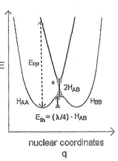
electronic states are energetically indistinguishable). In the case of transition metal

complexes, the experimental λ or “Eop” (as seen later in Figure 1.3) will arise both

from redox-state dependent structural shifts in the primary coordination sphere

(ligand set) and in the secondary/tertiary coordination spheres (or first and second

“hydration” shells) surrounding the reactant ions. Frequently it is assumed that the

total nuclear reorganizational energy, λ, can be apportioned into separate

“inner-sphere”, λ_in, and “outer-sphere”, λ_out, reorganizational energy contributions as

described below,

out in λ

λ

λ  (1-7)19, 23

where λ_Owould presumably capture all reorganization exterior to the ligand sphere.

The Gibbs activation free energy for the thermal ET process, __G*_{, is the}

energy required to reach transition state geometry through which reactants must pass

on their way to products. This energy has been shown by Marcus and Hush26-28 to be

(47)

12 2 r * λ G Δ 1 4 λ G _       

  (1-8)19, 22, 23

in the limit of linear solvent response to field fluctuations and strictly harmonic

free-energy surfaces.25, 29 Here Δ_rGis the driving force (if any) for reaction (equivalent

to the “standard reaction Gibb’s free energy change” or ΔE1/2 as measured

electrochemically). Equation (1-8) follows from the assumption of parabolic

(harmonic) potential/free-energy surfaces as defining the shape of the reaction

coordinate (with negligible departure due to resonance interactions) and in the limit of

negligibly small changes in the harmonic oscillator force constants (of all relevant

modes) upon going from [D,A] to [D ,A-]_.12, 26, 30_{The activation free energy can}

also be apportioned into inner- and outer-sphere components by applying equation

(1-7) to equation (1-8) and thus,

* out *

in

* _G _G

G  

 (1-9)

where *

in

G

 is the inner-sphere (skeletal) part of the Gibbs activation energy and

* out

G

 is the (presumably separable) outer-sphere (solvent) part. For ET

self-exchange reactions such as the ones to be discussed here, the [D,A] and [D ,A-]

ground state species are thermodynamically indistinguishable, therefore _Δ_G

r is

necessarily zero and equation (1-8) simplifies to,

4

(48)

13

1.4.1 The “inner-sphere” reorganizational energy, λin

In the case of ET between transition metal complexes, the “inner-sphere”

reorganizational energy, λ_in, can sometimes be treated in an especially simple way if

the reactant complexes contain identical small (or even mono-atomic) ligands which

then carry the bulk λ_in simply in the metal-ligand equilibrium bond distance changes

attending ET at each metal center. In such cases, λ_in can be expressed as,

) ( 2 ) d ( n 2 1 2 2 1 f f f f in _   

 (1-11)22

where n is the number of identical ligands coordinated to one of the reactant metals

(typically six), f₁ and f₂ are the symmetric stretching force constants for these

modes in the two different redox states at the metal center and d_ is the difference

between the equilibrium metal-ligand bond distances in the two different redox states

(as typically measured on separated reactant ions by crystallography). This

expression for the inner-sphere reorganization energy is a highly simplified model in

which the reactants are treated as two roughly spherical complexes with only one

specific force constant being ascribed to each reactant ion. A more realistic portrayal

of the inner-sphere reorganization energy encompasses the summation over all

intramolecular vibrations of each complex involved in the reaction which change

upon ET. In this more general approach, λ_in is described by,



 



i

i i in f ( d )2

2 1

(49)

14

where f_i = 2 f₁ f₂/( f₁+ f₂) and is the “reduced” force constant for the ith

inner-sphere vibration, and (d_)_i is the difference in the equilibrium metal-ligand bond

distances in the two oxidation states.

1.4.2 The “outer-sphere” (solvent) reorganzational energy, λout

The energy required to reorganize the medium outside of the primary

coordination spheres of the reactant ions is defined as the “outer-sphere”

reorganziational energy, λ_out. It is related to the change in solvation due to solvent

dipole electrostriction, orientation, libration, and other effects which contribute to the

overall λ for reaction.31 Generally, the reactant with the higher charge (the species

“A” in our notation thus far but soon to be specified as “RuIII”) is more strongly

solvated by the polar solvent molecules than its partner in the encounter complex, and

this leads to significantly different degrees of polarization of the solvent medium

exterior to the primary ligand sphere around A.

In the early model developed by Marcus and Hush, the medium outside of the

inner-coordination sphere was treated as a “dielectric continuum” with two

identifiable parts of the total polarization response assumed separable on the basis of

their respective timescales. The rapid, smaller portion of the response was ascribed to

the electronic polarizability of the molecules of the medium, and the slow, larger

portion to the vibration-libration-orientation polarization of the molecular dipoles of

the medium.23 They used the fact that the rapid electronic polarizability of the

(50)

15

realization was that this “optical-frequency” electronic polarizability of the medium

remains in equilbrium with the electrostatic change accompanying an ET event, while

the slow vibration-orientaition polarization of the medium has to fluctuate/adjust to a

non-equilibrium value appropriate to the “averaged” charge distribution of the

activated complex prior to a thermally-activated ET event. This is the constraint

which governs whether the electronic ET transition is “allowed” within the

zero-Franck-Condon energy or “isoenergetic” requirement for the elementary ET step.12, 32

The free-energy change necessary to produce the non-equilibrium polarization of the

solvent appropriate to the transition state when the reactants are treated as spheres

was then independently derived by Marcus and Hush as,

                 s 2 2 1 2 out D 1 n 1 d 1 r 2 1 r 2 1 ) (

λ e (1-13)12, 23, 26, 27

where e is the amount of charge transferred in the reaction, r₁ and r₂ are the radii

of the two reactant complexes, d is the distance between the centers of the two

reactants, n is the refractive index (which upon squaring gives the “optical” dielectric

constant, D ), and _op D is the “static” dielectric constant of the medium (which _s

describes the ability of any solvent or other condensed medium to screen electric

fields at low frequency). In our case n2 is 5.533 and D is 78.5 at 298 K for water _s

(negligibly different at 298 K for D2O) . Equation (1-13) is rigorously valid only if,

) r (r

d ₁ ₂ (1-14)

which implies that the “contacting spheres” idea is actually outside the range of