Surfing the Index of Consumer Sentiment: Identifying Statistically Significant Monthly and Yearly Changes

211

Surfing the Index of Consumer Sentiment:

Identifying Statistically Significant

Monthly and Yearly Changes

Paul R. Yarnold, Ph.D.

Published monthly by the Survey Research Center of the University of Michigan, the Index of Consumer Sentiment (ICS) is widely followed, and one of its factors (the Index of Consumer Expectations) is used in the Leading Indicator Composite Index published by the US Depart-ment of Commerce, Bureau of Economic Analysis.1 Using household telephone interviews the ICS provides an empirical measure of near-term consumer attitudes on business climate, and personal finance and spending.2 Variation in ICS influences price and volume in currency, bond, and equity markets in the US and in markets globally.3 The practice of releasing monthly ICS values five minutes to two seconds earlier for elite customers via high-speed communication channels was recently suspended because it provided unfair trading advantages. This article investigates the trajectory of the ICS over the most recent three-years, evaluating the statistical significance of month-over-month and year-over-year changes. These analyses define a longitudinal series of class variables which may be modeled temporally using time-lagged single- (UniODA) and multiple- (CTA) attribute ODA methods.

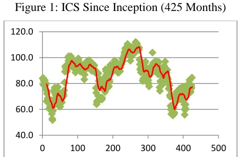
Figure 1 is an illustration of the raw ICS series since inception January 1, 1978, through May 1, 2013 (a total of 425 sequential months). The one-year moving average, shown in red, has been beneath the index value—set to equal 100 in 1966, over most of the series. An index value is used to initiate the series (the starting value is arbitrary), but does not address variability in the series. In Figure 1 (and Figure 2) the 100th ICS value occurs on April 1, 1986; the 200th on Au-gust 1, 1994; the 300th on December 1, 2002; and the 400th on April 1, 2011.

Figure 1: ICS Since Inception (425 Months)

40.0 60.0 80.0 100.0 120.0

212 Because this is a longitudinal series the

data are ipsatively standardized.4,5 The formula for ipsative and normative standardization is: zi=(Xi – Mean)/SD, where zi is the z-score for

the ith observation in the series, and Xiis the raw

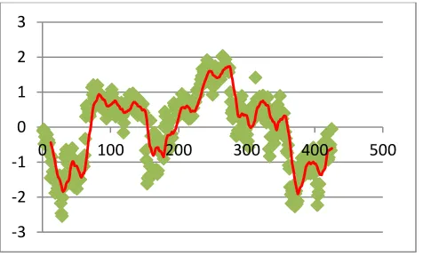
score for the ith observation. In normative stand-ardization Mean and SD are computed based on a sample of observations assessed at a single point in time, whereas in ipsative standardiza-tion Mean and SD are computed based on a sin-gle observation assessed on multiple points in time.6,7 The ipsative z-score indicates the mag-nitude of the ith observation (score) relative to all of the observations (scores) in the series. For the ICS series, Mean=85.2 and SD=13.2. Figure 2 presents the ipsatively standardized ICS series and 12-month moving average, which as seen closely resembles the raw data ICS series viewed across time (Figure 1).

Figure 2: Ipsatively Standardized ICS Since Inception (425 Months)

Despite their similar appearances, the ipsative series is more informative than the raw data series, because the former takes the vari-ance between observations into consideration, whereas the latter does not account for variabil-ity. For example, Figure 2 reveals that the moving average has been above the mean value of the ICS assessed twice since inception, once between days 65 and 150 of the series, and again between days 200 and 360 of the series.

While a historical analysis of the entire series is of course interesting, the present study focuses on more recent trajectory—the past three years are considered. For the 36-month ICS series, Mean=72.6 and SD=6.5. Figure 3 presents a scatter plot of the ipsative ICS series over the most recent 36 months, and Figure 4 presents the same information with a line plot: both illustrate the 12-month moving average.

Figure 3: Scatter Plot of Ipsative ICS Score: Most Recent 36 Months

Figure 4: Line Plot of Ipsative ICS Score: Most Recent 36 Months

Evaluating Year-Over-Year Changes

In the first exploration of the recent ipsative ICS series, UniODA8 is used to assess each of 13 year-over-year comparisons that exist for data in Figure 3. The analysis is called a forward-stepping little jiffy with a bin width of

-3 -2 -1 0 1 2 3

0 100 200 300 400 500

-3 -2 -1 0 1 2 3

0 10 20 30 40

-3 -2 -1 0 1 2 3

213 24 months: the first half (more dated) of the

ipsative ICS scores in each analysis are statisti-cally compared with the second (more recent) ipsative ICS values.9 The results of these anal-yses are summarized in Table 1: changes indi-cated as UP were statistically significant at the generalized criterion; changes indicated in red

were significant at the experimentwise criterion.

Table 1: Summary of UniODA Analysis of 13 Year-Over-Year Changes in Ipsative ICS Score

Year Ending

Change in

Annual zICS ESS ESP

May 2013 Up 58.3 70.6

April 2013 Up 58.3 70.6

March 2013 Up 66.7 75.0

February 2013 Up 75.0 80.0

January 2013 Up 75.0 80.0

December 2012 Up 75.0 80.0

November 2012 Up 58.3 70.6

October 2012 None 50.0 51.1 September 2012 None 41.7 42.0 August 2012 None 33.3 33.3

July 2012 None 33.3 44.4

June 2012 None 41.7 63.2

May 2012 None 41.7 63.2

As seen the ipsative ICS series did not have a statistically significant (p<0.05) year-over-year change from May through October of 2012, and during this period the accuracy of the UniODA model (indexed by ESS) was in the moderate range with the exception of October— which exactly met the criterion for a relatively strong effect.8 In November of 2012 the first year-over-year increase in ipsative ICS score in the series occurred (a relatively strong effect), but it was statistically significant only at the generalized criterion. In the following three months, December of 2012 through February of 2013, statistically significant increases occurred (p<0.05, experimentwise criterion), and all three models exactly met the criterion for a very

strong effect.8 Finally, the most recent three months continue to show sustained, relatively strong, statistically significant year-over-year increases in ipsative ICS score, but only when considered at the generalized criterion.

The little jiffy analysis just performed treated all of the year-over-year comparisons as being of equal importance, in the sense that the Sidak Bonderroni-type multiple comparisons criterion that was used to assess experimentwise statistical significance8 was not a sequentially-rejective procedure, but instead was computed based on all the tests of statistical hypotheses conducted. However, it is also possible to focus the analysis on the earliest part of the series (and use a forward-stepping little jiffy), on the most recent part of the series (and use a back-ward-stepping little jiffy), or on any specific location within the series (and use a forward- and/or backward-stepping little jiffy), by selecting the theoretical perspective and corre-sponding little-jiffy analytic approach that focuses statistical power on the specific com-parisons which are of primary interest to the researcher.9,10

214 Evaluating Month-Over-Month Changes

While the year-over-year changes in the ipsative CSI series are of interest to longer-term investors, short-term traders focus on more re-cent and more granular time horizons. For ex-ample, were the CSI updated every hour using a different random set of respondents, then hourly changes in the index would be of greatest inter-est to short-term traders (if the present study had been an analysis of the temporal trajectory of an individual investment instrument which is traded in real-time—such as a common stock, bond, or commodity, then a variety of time- and/or volume-based binning strategies could be used to define series for analyses conceptually consistent with series presented herein).

UniODA has been successfully used to analyze data for small samples, but comparing one month versus another month statistically is not possible using ODA methods.11 Instead, sta-tistical methods have been developed on the basis of classical test theory7 which are used for analyzing data from a single-case “N-of-1” se-ries involving a relatively small number of ob-servations. Designs which may be analyzed via this method involve a single observation (series or subject) assessed on multiple variables at a single point in time; measured on a single varia-ble that is assessed at multiple points in time; or measured on multiple attributes assessed at multiple points in time.12-14

In the N-of-1 classical test theory-based methodology, the ipsative z-score for the ith ob-servation (i.e., time, testing or measurement pe-riod) is subtracted from the ipsative z-score for the following i+1th observation: if the difference is positive then the more recent (i+1th) meas-urement was greater than the less recent (ith) measurement; if the difference is negative then the opposite is true; and if the difference is zero then the two measurements were identical. The absolute value of the difference between the two ipsative z-scores is compared against a critical difference (CD) score, which is a function of the lag-1 autocorrelation coefficient7,14 [ACF(1)] for

the data in the series; the number of inter-score comparisons which are being conducted (J); and the z-score corresponding to the desired experi-mentwise Type I error (p) level, taking into con-sideration if analyses are one- or two-tailed (for one-tailed p<0.05, z= 1.64; for two-tailed p<0.05, z=1.96).15 CD is computed as CD=z(J[1-ACF(1)])½.

In the present application ACF(1)=0.742 (p<0.0001), and a total of 35 month-over-month two-tailed comparisons are to be evaluated. Thus CD=1.96*(35*(1-0.742))½=5.89. The CD score is massive due to the large number of tests of statistical hypotheses which are conducted (35). None of the month-to-month absolute dif-ferences in ipsative CSI score were as large as the CD score, indicating the absence of any statistically significant effects at the experi-mentwise criterion.

If one instead used the generalized “per-comparison” criterion, the value 1 is used in the formula for CD rather than 35 (indicating one test of a statistical hypothesis), and CD=1.96* (1*(1-0.742))½=0.996. Presently, six of the month-over-month differences were as large or were larger than this CD score, indicating the presence of a statistically reliable month-over-month change at the generalized criterion. The six significant month-over-month changes which occurred are given in Table 2.

Table 2: Month-Over-Month Differences in Ipsative ICS Score with Generalized p<0.05

Month i Month i+1 zi+1 – zi

1 (6/1/2010) 2 (7/1/2010) -1.27 9 (2/1/2011) 10 (3/1/2011) -1.55 13 (6/1/2011) 14 (7/1/2011) -1.21 14 (7/1/2011) 15 (8/1/2011) -1.22 30 (11/1/2012) 31 (12/1/2012) -1.52 35 (4/1/2013) 36 (5/1/2013) 1.25

215 significant month-over-month changes are read-ily seen. The five significant monthly declines occurred after months 1, 9, 13, 14 and 29. And, the only statistically significant rise in the ip-sative ICS score over this series occurred in the most recent measurement, after week 35.

Conducting Inferential Statistical Analysis of Factors Affecting Statistically Reliable

Temporal Changes in the Series

Findings of analyses conducted within series as done herein are of paramount interest to some people, yet in a sense these findings re-flect the beginning of the analytic enterprise. If the subject of the investigation—here the ICS score—never changed across time then it would be a constant and statistical analysis would be impossible. However sometimes the series moves significantly up or down over time, whether compared in longer (year-over-year) or shorter (month-over-month) time perspective. In Table 1, for example, when the series increases it may be dummy-coded as 1, and when the series does not change it may be dummy-coded as a 0. In this manner, any sequential analysis such as reported herein defines a serial class variable. Factors (attributes) may be used to dis-criminate between these 0’s and 1’s, using UniODA8 or it’s BIG DATA software equiva-lent MegaODA16,17 to analyze univariate rela-tionships, and CTA18 to analyze multivariate relationships. For example, potential attributes which could be evaluated as possible predictors of ipsative ICS scores at time i might include the most recent ipsative scores at time i or time i-1 for unemployment rate, political turmoil affecting financial matters, threat of war, Federal Reserve Board activity, 30-year interest rates, and so forth.

References

1

http://research.stlouisfed.org/fred2/series/UMC SENT/

2

Howrey EP (2001). The predictive power of the Index of Consumer Sentiment. Brookings Pa-pers on Economic Activity, 1, 175-216.

3

Golinelli R, Parigi G (2004). Consumer senti-ment and economic activity: A cross country comparison. Journal of Business Cycle Meas-urement and Analysis, 1, 147-172.

4

Yarnold PR, Soltysik RC (2013). Ipsative transformations are essential in the analysis of serial data. Optimal Data Analysis, 2, 94-97.

5

Yarnold PR (2013). Ascertaining an individual patient’s symptom dominance hierarchy: Analy-sis of raw longitudinal data induces Simpson’s Paradox. Optimal Data Analysis, 2, 159-171.

6

Yarnold PR, Feinglass J, Martin GJ, McCarthy WJ (1999). Comparing three pre-processing strategies for longitudinal data for individual patients: An example in functional outcomes research. Evaluation in the Health Professions, 22, 254-277.

7

Yarnold PR. Statistical analysis for single-case designs. In: FB Bryant, L Heath, E Posavac, J Edwards, E Henderson, Y Suarez-Balcazar, S Tindale (Eds.), Social Psychological Applica-tions to Social Issues, Volume 2: Methodologi-cal Issues in Applied Social Research. New York, NY: Plenum, 1992, 177-197.

8_{Yarnold PR, Soltysik RC (2005). Optimal data} analysis: Guidebook with software for Windows. Washington, D.C.: APA Books.

9

Yarnold PR (2013). Statistically significant increases in crude mortality rate of North Da-kota counties occurring after massive environ-mental usage of toxic chemicals and biocides began there in1998: An optimal static statistical map. Optimal Data Analysis, 2, 98-105.

10

an-216 nual crude mortality rate most recently began

increasing in McLean County, North Dakota. Optimal Data Analysis, 2, 143-147.

11

Yarnold PR (2013). UniODA and small sam-ples. Optimal Data Analysis, 2, 71.

12

Yarnold PR (1982). On comparing interscale difference scores within a profile. Educational and Psychological Measurement, 42, 1037-1045.

13

Yarnold PR (1988). Classical test theory methods for repeated-measures N=1 research designs. Educational and Psychological Meas-urement, 48, 913-919.

14

Mueser KT, Yarnold PR, Foy DW (1991). Statistical analysis for single-case designs: Eval-uating outcomes of imaginal exposure treatment of chronic PTSD. Behavior Modification, 15, 134-155.

15

An excellent z-score calculator is available at: http://www.measuringusability.com/pcalcz.php

16

Soltysik RC, Yarnold PR (2013). MegaODA large sample and BIG DATA time trials: Sepa-rating the chaff. Optimal Data Analysis, 2, 194-197.

17

Soltysik RC, Yarnold PR (2013). MegaODA large sample and BIG DATA time trials: Har-vesting the Wheat. Optimal Data Analysis, 2, 202-205.

18

Soltysik RC, Yarnold PR (2010). Automated CTA software: Fundamental concepts and con-trol commands. Optimal Data Analysis, 1, 144-160.