Journal of Industrial Engineering and Management Studies
Vol. 3, No. 2, pp. 17-32 www.jiems.icms.ac.ir
Improving the performance of financial forecasting using different
combination architectures of ARIMA and ANN models
Z. Hajirahimi1,*, M. Khashei1
Abstract
Despite several individual forecasting models that have been proposed in the literature, accurate forecasting is yet one of the major challenging problems facing decision makers in various fields, especially financial markets. This is the main reason that numerous researchers have been devoted to develop strategies to improve forecasting accuracy. One of the most well established and widely used solutions is hybrid methodologies that combine linear statistical and nonlinear intelligent models. The main idea of these methods is based on this fact that real time series often contain complex patterns. So single models are inadequate to model and process all kinds of existing relationships in the data, comprehensively. In this paper, the auto regressive integrated moving average (ARIMA) and artificial neural networks (ANNs), which respectively are the most important linear statistical and nonlinear intelligent models, are selected to construct a set of hybrid models. In this way, three combination architectures of the ARIMA and ANN models are presented in order to lift their limitations and improve forecasting accuracy in financial markets. Empirical results of forecasting the benchmark data sets including the opening of the Dow Jones Industrial Average Index (DJIAI), closing of the Shenzhen Integrated Index (SZII) and closing of standard and poor’s (S&P 500) indicates that hybrid models can generate superior results in comparison with both ARIMA and ANN models in forecasting stock prices.
Keywords: Combination Architecture, Hybrid Model, Artificial Neural Networks (ANNs),
Auto-regressive Integrated Moving Average (ARIMA), Forecasting Stock Price.
1. Introduction
because the underlying process cannot easily be determined. The motivation of using hybrid models comes from this assumption that either one single model cannot identify the true data generation process or single models may not be totally sufficient to identify all the characteristics of the data.
In the literature of time series forecasting, several linear classical approaches have been proposed. Autoregressive integrated moving average (ARIMA) models are one of the most important and widely used linear time series models. The popularity of the ARIMA model comes from its statistical features as well as the well-known Box-Jenkins (1976) methodology in the model building process. In addition, ARIMA models can implement various exponential smoothing models. Although the ARIMA model has advantages of accurate forecasting over a short period and ease of implementation, its main limitation is the pre-assumed linear form of the model. Artificial neural networks (ANNs) are one of the most important models among nonlinear intelligent models. The major advantage of neural networks is their flexible nonlinear modeling capacity. In artificial neural networks, no longer need to specify the form of the particular model. Moreover, the model is adaptively formed based on the features presented from the data. Because of the capacity of these models in nonlinear modeling, they have been frequently used in several studies for building hybrid models. Of course, it must be noted that although both ARIMA and ANN models can respectively achieved successes in their own linear or nonlinear domains, none of them is a universal approach that can be generally applied in all circumstances. The approximation of the ARIMA to model the complex nonlinear problems may be inadequate. Moreover, using ANNs to model linear problems have yielded mixed results. Hence, it is not wise to apply ANNs blindly to any type of data.
Hybrid ARIMA/ANN models can be divided into three main architectures. In the first and second classes of hybrid ARIMA/ANN models, a time series is considered to be composed of a linear and nonlinear components. While in third category, a combined forecasting is calculated based on a linear combination of each forecasting model result. In this paper, in order to improve forecasting accuracy in financial markets, three combination architectures of ARIMA and ANN models are presented. To evaluate performance of hybrid models and their improvements against individual models, three benchmark data sets of financial markets are elected. The rest of this paper is organized as follows: in section 2, the literature of hybrid models is briefly reviewed. In the section 3, basic concepts and modeling procedures of ARIMA and ANN models for time series forecasting is introduced. In section 4, the three combination methodologies of ARIMA and ANN models are descripted. The description of used benchmark data set and obtained results of three hybrid models are presented in section 5. In section 6, the performance of models in forecasting benchmark data sets of stock prices, including the Dow Jones Industrial Average Index (DJIAI), closing of the Shenzhen Integrated Index (SZII) and closing of standard and poor’s (S&P 500) is compared together. Section 7 contains the concluding remarks.
2. Literature review
combining fuzzy systems and ANNs model for forecasting Tehran stock index. Kristjanpoller &Minutolo (2015) presented a hybrid model, including ANN and GARCH models for forecasting gold price. Xiong et al. (2017)proposed a hybrid modeling framework combining interval Holt’s exponential smoothing method and multi-output support vector regression (MSVR) for time series forecasting. Yuan et al. (2017) proposed a hybrid autoregressive fractionally integrated moving average (ARFIMA) and least square support vector machine (LSSVM) model to forecast short-term wind power.
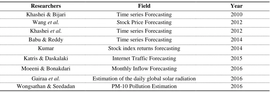
In recent years, several hybrid models incorporating ARIMA and ANN models presented in the literature of time series forecasting in order to take special advantages of these models in linear and nonlinear modeling respectively and overcoming their limitations. Zeng et al. (2008) proposed a hybrid ARIMA/ANN model to forecast traffic flow. Aladage et al. (2009) constructed a hybrid model incorporating Elman's recurrent neural networks and ARIMA models. Areekul et al. (2010) used the combination of ARIMA and multilayer perceptrons for short-term price forecasting. Shafie-khah (2011) proposed a hybrid model based on the ARIMA and the radial basis function neural network (RBFNs) and used it to forecast electricity price. The literature of hybrid models incorporating ARIMA and ANN models are summarized in Table 1.
Although in past two decades, various attempts have been made to use hybrid models in different fields, all of this studied have been focused on the improving accuracy of forecasting by one hybrid combination method. Thus, in this paper firstly the combination architecture of individual models such as ARIMA and ANN models is categorized in three main classes and then proving this issue that combining different models are often yield of the superiority in forecasting performance in stock price forecasting.
3. The Autoregressive Integrated Moving Average and Artificial Neural
Networks Models
In this section, basic concepts and modeling procedures of autoregressive integrated moving average (ARIMA) and artificial neural networks (ANNs) for time series forecasting is briefly introduced.
3.1.Autoregressive Integrated Moving Average (ARIMA) Models
In the autoregressive integrated moving average (ARIMA) models, the future value of the variable is assumed to be a linear function of past values and error terms.
t t 1 t 1 p t p t 1 t 1 q t q
y u φ y ... φ y ε θ ε ... θ ε (1)
where, ytis the actual value at time t,εt is the white noise which assumed to be independently
and identically distributed with a mean of zero and constant variance of σ2. p and q are the
integer numbers of autoregressive and moving average terms in ARIMA model,
i
φ ( i 1,2 ,...., p ) and θ ( j 1, 2 ,....,q )i are the model parameters to be estimated. The Box-Jenkines methodology always includes three iterative steps of model identification, parameter estimation and diagnostic checking.
3.2. Artificial neural networks (ANNs)
parallel processing of the information from the data. No prior assumption of the model form is required in the model building process. Instead, the network model is largely determined by the characteristics of the data. Single hidden layer feed forward network (also known as multilayer perceptrons) is the most widely used model form for time series modeling and forecasting. In this paper, this type of neural network is used for all nonlinear modeling. The relationship between the output ( yt ) and the inputs ( yt 1 ,...., yt p ) in multilayer perceptrons has the following
mathematical representation (khashei and Bijari, (2010)).
q p
t 0 j 0 , j i , j t i t
j 1 i 1
y w w .g [w w .y ]
(2)where, wi , j( i 0 ,1...., p , j 1 , 2 ,....,qand w ( jj 0 ,1 , 2...,q ) are model parameters often called connection weights; p is the number of input nodes; and q is the number of hidden nodes.
Hence, the multilayer perceptron model presented in Eq. (2), in fact, performs a nonlinear functional mapping from past observations to the future valueyt, i.e.
t t 1 t 2 t p t
y f ( y , y ,...., y ) (3)
Where, w is a vector of all parameters and f is a function determined by the network structure and connection weights. Thus, the neural networks are equivalent to a nonlinear autoregressive model. The process of choosing parameters in different layers is described as follows:
Input layer phase: For the time series problems, a MLP is fitted with past lagged value of actual
data (yt 1 ,..., yt p ) as an input vector. Therefore, input layer is composed of p nodes that are
connected to the hidden layer.
Hidden layer phase: The hidden layer is an interface between input and output layers. The MLPs model which are designed in this paper have a single hidden layer with q nodes. In this step, one of the important tasks is determining the type of activation function (g) which is identifying the relationship between input and output layer. Neural networks support a wide range of activation function such as linear, quadratic, tanh and logistic. The logistic function is often used as the hidden layer transfer function that are shown in Eq. (4).
1 g ( x )
1 exp( x )
(4)
Output layer phase: In this step, by selecting an activation transfer function and the appropriate number of nodes, the output of neural network is used to predict the future values of time series. In this paper output layer of designed neural networks contains one node because the one –step-ahead forecasting is considered. Also, the linear function as a non-linear activation function is introduced for the output layer. The formula of relationship between input and output layer is presented in Eq. (2).
4. Three Architecture of Hybrid Autoregressive Integrated Moving Average
(ARIMA) and Artificial Neural Network (ANN)
In the literature of time series forecasting, several hybrid models are proposed. Hybrid methodologies that combine linear and nonlinear models together are one the most popular solution for capturing different aspects of the underlying patterns in data and improving forecasting accuracy. Thus, in this paper, three architectures of hybrid ARIMA/ANN models are presented in the next section.
Table 1. The literature of ARIMA/ANN hybrid model
4.1 Combination Architecture-1
In the first stage of combination architecture-1, the ARIMA model is used to capture the linear component. Let et denote the residual of the ARIMA model at time t, then:
t t ˆt
e y L (5)
where, the ˆLt is the forecasting value at time t which is obtained by ARIMA model. Then in the
second stage, by modeling residuals using ANN, nonlinear relationships can be discovered. With
n input nodes, the ANN model for the residuals will be:
t t 1 t 2 t n t ˆt ˆt t 1 t 2 t n
e f ( e ,e ,...,e ) N e f ( e ,e ,...,e ) (6)
where, f is a nonlinear function determined by the ANN model, Nˆt is the forecasting value at time t which is obtained by ANN model and εt is the random error. The framework of
combination architecture-1 is displayed in Fig. (1). Note that if the model f is an inappropriate
one, the error term is not necessarily random. Therefore, the correct identification is critical. In this way, the combined forecast will be as follows:
t ˆt ˆt
ˆy L N (7)
Year Field
Researchers
2010 Time series Forecasting
Khashei & Bijari
2012 Stock Price Forecasting
Wang et al.
2012 Time series Forecasting
Khashei et al.
2014 Time series Forecasting
Babu & Reddy
2014 Stock index returns forecasting
Kumar
2015 Internet Traffic Forecasting
Katris & Daskalaki
2016 Monthly Inflow Forecasting
Moeeni & Bonakdari
2016 Estimation of the daily global solar radiation
Gairaa et al.
2016 PM-10 Pollution Estimation
4.2. Combination Architecture-2
The combination architecture-2 also has two main stages. In the first stage, ANN model is used in order to model the nonlinear part of time series. Let etdenote the residual of ANN model at
time t, then:
t t ˆt
e y N (8)
where, ˆNt is the forecasting value at time t which is obtained by ANN model. Then ARIMA model is used to model residuals of the ANN model in order to analyze the linear patters. In this way, the ARIMA model with m lags for the residuals will be:
t t 1 t 2 t m t ˆt ˆt t 1 t 2 t m
ef ( e ,e ,...,e ) L e f ( e ,e ,...,e ) (9)
where, f is a linear function determined by the ARIMA, t
ˆL is the forecasting value for time t
from the ARIMA model on the residual data, and tis the random error. The framework of MLP-ARIMA model is displayed in Fig. (2). In this way, the combined forecast will be as follows:
t ˆt ˆt
ˆy LN
(10)
Time series
ARIMA
Predicted
value ANN
t
ˆL Nˆt
Integrated prediction
t
e
Figure1. the framework of combination architecture -1
Time series
ANN
Predicted
value ARIMA
t
ˆ N
Integrated prediction
t
e
t
ˆL
4.3. Combination Architecture-3
In this method, the ARIMA and ANN models are employed to analyze the linear and nonlinear components in the data simultaneously and then two forecasting results are obtained. By multiplying optimal weight coefficients of two forecasting results and adding them up, the final forecasting can be obtained by Eq.(11). Where f ( iit 1 , 2 ,..., m ) are the forecasting results that
are obtained from i-th forecasting model at time t, m are the number of individual model and wi
is the weight coefficient for the i-th forecasting method.
m
t i it
i
ˆ
ˆy w f
1
(11)
The forecasting error are computed from Eq. (12).
m m m m
t t t i t i it i t it i it i 1 i 1 i 1 i 1
ˆ ˆ
ˆ
e y y w y w f w ( y f ) w e
(12)By using ARIMA and ANN models Eq. (13) can be rewrite as follow
t 1ˆt 2 ˆt
ˆy w L w N (13)
Whereˆyt , ˆLt and Nˆt are the forecasting value of hybrid, ARIMA and ANN models respectively. Moreover the weights are allocated to each model are estimated from ordinary least squares method and computed from Eq. (14) and (15). The framework of combination architecture -3 is displayed in Fig. (3).
n n n n
2
t t t t t t t
t 1 t 1 t 1 t 1
1 n n n
2 2 2
t t t t
t 1 t 1 t 1
ˆ ˆ ˆ ˆ ˆ
N L y L N N y
W
ˆ ˆ ˆ ˆ
L N ( L N )
(14)n n n n
2
t t t t t t
t 1 t 1 t 1 t 1
2 n n n
2 2 2
t t t t
t 1 t 1 t 1
ˆ ˆ ˆ ˆ ˆ
L N y L N L y
W
ˆ ˆ ˆ ˆ
L N ( L N )
(15) Time series ANN Predicted value ARIMA Integrated prediction Predicted value t ˆN ˆLt
5
.
Appling three Architectures of Hybrid ARIMA/ANN Models for Stock Price
Forecasting
In this section, three abovementioned hybrid models are applied for stock price forecasting. The benchmark data sets including the opening of the Dow Jones Industrial Average Index (DJIAI), closing of the Shenzhen Integrated Index (SZII) and closing of standard and poor’s (S&P 500) are chosen for this purpose. The description of data sets, the procedure of hybrid models and designed models for forecasting benchmark data sets are briefly presented in the next subsections
5.1. Dow Jones Industrial Average Index (DJIAI) data set
The Dow Jones Industrial Average Index data set contains stock opening prices from the January 1991 to the December 2010 and totally has 240 monthly values. The plot of the DJIAI data set is show in the Figure 4. The first 180 values (about 75% of the sample) are used as training sample and the remaining 60 values are applied as test sample.
Figure4. the monthly DJIAI stock opening prices from January 1991 to December 2010
2000 3500 5000 6500 8000 9500 11000 12500 14000
0 25 50 75 100 125 150 175 200 225
5.1.1. The architecture -1
Stage I: (Linear modeling): In the first stage of the combination architecture-1, by using Eviews
software, the best-fitted model is ARIMA 1 , 2 ,0
.Stage II: (Nonlinear modeling): In order to analyze the obtained residuals from the previous stage
and based on the concepts of ANN models, in MATLAB software, the best fitted model composed of five inputs, three hidden and one output neurons (in abbreviated form N( 5 ,3 ,1 )), is designed.
Stage III: (Combination): In the last stage, obtained results from stage I and II are combined together.
The estimated values of the combination architecture-1 against actual values for all data are plotted in Figure 5.
5.1.2. The architecture-2
Stage I: (Nonlinear modeling): In the first stage of the architecture-2, in order to capture nonlinear
patterns of time series a multilayer perceptron with three inputs, three hidden and one output neurons (in abbreviated form N( 3 ,3 ,1 )), is designed.
Stage II: (Linear modeling): In the second stage of the architecture-2 hybrid model, obtained
residuals from previous stage are treated as the linear model. Thus, considering lags of the ANN residuals as input variables of the ARIMA model, the best fitted model is ARIMA 3 ,0 ,3
.Stage III: (Combination): In the last stage, obtained results from stage I and II are combined together.
The estimated values of the combination architecture-2 against actual values for all data are plotted in Figure 6.
5.1.3. The architecture-3
Stage I: (linear and nonlinear modeling) Due to the basic concepts of ARIMA and ANN models in
forecasting, the best fitted ARIMA and ANN models that are designed in Eviews and MATLAB
software respectively are ARIMA 1 , 2 ,0
and one layer neural network composed of three inputs, three hidden and one output neurons (in abbreviated form (N( 3 ,3 ,1 )). It should be noted that different network structures are examined to compare MLPs performance and the best architecture are selected which presented the best forecasting accuracy with the test data.Stage II: (initializing weights) In this step the optimum weights of predicted value that are obtained
from previous stage, are determined. Two weights are estimated by linear regression model with OLS approach in Eviews software.
Stage III: (final forecasting) By multiplying two optimal weight coefficients to obtain forecasts from
Figure5.Estimated values of the combination architecture-1 for DJIAI
Figure6.Estimated values of the combination architecture-2 for DJIAI
2000 3500 5000 6500 8000 9500 11000 12500 14000
5 30 55 80 105 130 155 180 205 230
Actual Value Estimated Value
2000 3500 5000 6500 8000 9500 11000 12500 14000
5 30 55 80 105 130 155 180 205 230
Actual Value Estimated Value
2000 4000 6000 8000 10000 12000 14000
5 30 55 80 105 130 155 180 205 230
5.2. Closing of the Shenzhen Integrated Index (SZII) data set
The Shenzhen Integrated Index (SZII) data set covers from January 1993 to December 2010 and totally has 216 monthly observations. The plot of this data set is shown in Fig. (8). The first 168 data are used as training sample and the remaining 48 data are applied as test data set.
Figure8 .The monthly SZII stock closing prices from January 1993 to December 2010.
5.2.1. The architecture -1
According to the modeling procedure of architecture combination-1, for linear modeling, by using
reviews software, the best fitted model is an ARIMA (1,0,0). Then in nonlinear modeling, the neural network composed of four inputs, four hidden and one output neuron, is designed. The estimated values of the combination architecture-2 against actual values for all data are plotted in Fig. (9).
4.2.1. The architecture -2
In a similar fashion, for nonlinear modeling, a neural network with three inputs, two hidden and one output neuron is designed. Then in the second stage, the best fitted model is an ARIMA (2,0,2) for capturing linear patterns in residuals. The estimated values of the combination architecture-2 against actual values for all data are plotted in Fig. (10)
4.2.1. The architecture -3
Due to the basic concepts of ARIMA and MLP models and according to the modeling procedure of architecture combination-3, the best fitted ARIMA and ANN models are ARIMA (1,0,0) and one layer neural network composed of three inputs, two hidden and one output neuron. Then optimal weights are calculated based on the OLS approach in Eviews software. The estimated values of the combination architecture-3 against actual values for forecasting SZII data set are plotted in Fig. (11).
0 3000 6000 9000 12000 15000 18000 21000 24000
1 26 51 76 101 126 151 176 201
Figure9.Estimated values of the combination architecture-1for SZII
Figure10.Estimated values of the combination architecture-2 for SZII
Figure11.Estimated values of the combination architecture-3 for SZII
5.3. Closing of standard and poor’s (S&P 500) data set
The Standard and Poor’s 500 (S&P 500) index data set includes 2349 daily closing stock price from
0 3000 6000 9000 12000 15000 18000
5 30 55 80 105 130 155 180 205
Actual Value Estimated Value
0 3000 6000 9000 12000 15000 18000
5 30 55 80 105 130 155 180 205
Actual Value Estimated Value
0 3000 6000 9000 12000 15000 18000
5 30 55 80 105 130 155 180 205
5.3.1. The architecture -1
In the first stage, the best linear ARIMA model is (1,0,0) and for nonlinear modeling in the second stage the neural network with three inputs, five hidden and one output neurons are designed. The estimated values of the combination architecture-1 against actual values in forecasting S&P 500 data set are plotted in Fig. (13).
Figure13. Estimated values of the combination architecture-1 for S&P500
5.3.2. The architecture -2
In the S&P 500 data set forecasting with architecture-2, similar to previous sections, the best fitted neural network is N( 3 ,3 ,1 ) and then in linear modeling the best linear model is found to be
ARIMA( 3 ,0 ,3 ).The estimated values of the combination architecture-2 against actual values for S&P 500 forecasting data set are plotted in Fig. (14).
Figure14. Estimated values of the combination architecture-2 for S&P500
700 900 1100 1300 1500
8 263 518 773 1028 1283 1538 1793 2048 2303
Actual Value Estimated Value
700 900 1100 1300 1500
2 257 512 767 1022 1277 1532 1787 2042 2297
5.3.3. The architecture -3
Similar to previous sections, for capturing linear and nonlinear patters in the data of S&P 500 simultaneously, the ARIMA( 1 ,0 ,0 ) and the neural network with three inputs, three hidden and one output neurons are designed. The optimum weights are obtained by OLS method. The estimated values of the combination architecture-2 against actual values of the forecasting SZII data set are plotted in Fig. (15).
Figure15. Estimated values of the combination architecture-3 for S&P500
6. Comparison of forecasting results
In this section, the predictive capabilities of three hybrid models are compared with their components −multilayer perceptrons and autoregressive integrated moving average− in three benchmark data sets. Two performance indicators, including mean absolute error (MAE), mean square error (MSE), which are computed from the following equations, are employed in order to compare forecasting performance of hybrid models and their components.
N
i i 1 1
MAE e
N
)16)
2N
i i 1 1
MSE e
N
)17)Forecasting results of hybrid models and their components for the DJIAI, SZII and S&P500 stock indexes in train and test data sets are summarized in Table (2) to (4) respectively. The numerical results of forecasting three benchmark data sets show that applying three hybrid models can improve
700 950 1200 1450 1700 1950
5 260 515 770 1025 1280 1535 1790 2045 2300
14.98% over than ARIMA model in the test data set. Moreover, the average improvement of three hybrid models in comparison with ANN model is 4.11% and 11.29% in MAE and MSE term and in comparison with ARIMA model is 4.89% and 17.63% of the test data set for forecasting DJII respectively.
Table 2. The performance of models for DJIAI in train and test data set
Models MAE MSE MAPE (%) SSE
train test Train test train test train test
ARIMA 245.69 369.84 119876 239015 3.19 3.56 21457866 14340936
ANN 231.23 366.80 107496 221930 3.01 3.04 19026914 13315798
Architecture -1 227.75 351.76 103822 204104.8 2.09 3.03 18272782 12246287
Architecture -2 229.49 358.41 105562 183310 2.09 3.03 18578914 10998646
Architecture -3 231.03 344.99 107447 203208 3.03 3/03 19018260 12192486
Table 3. The performance of models for SZII in train and test data set
Models MAE MSE MAPE (%) SSE
train test train test train test train test
ARIMA 224.45 1166.17 99255 2221776 7.30 10.26 16575670 106645281
ANN 215.38 1102.33 94577 1974479 7.08 9.08 15605205 94775037
Architecture -1 212.39 1083.88 91955 1915716 7.02 9.05 15080623 91954350
Architecture -2 210.91 1064.91 86221 1915422 7.02 10.01 14140258 91940270
Architecture -3 215.05 1074.87 94573 1928479 7.09 9.06 15604548 92566989
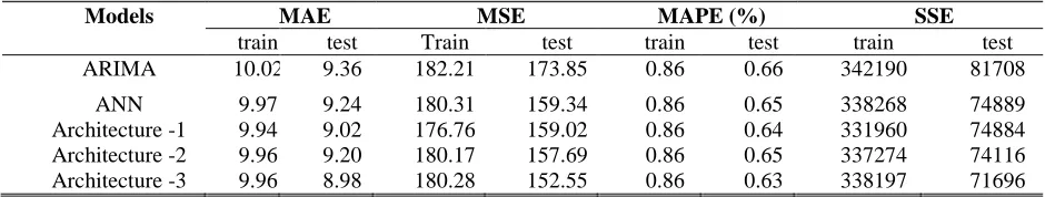
Table 4. The performance of models for S&P500 in train and test data set
Models MAE MSE MAPE (%) SSE
train test Train test train test train test
ARIMA 10.02 9.36 182.21 173.85 0.86 0.66 342190 81708
ANN 9.97 9.24 180.31 159.34 0.86 0.65 338268 74889
Architecture -1 9.94 9.02 176.76 159.02 0.86 0.64 331960 74884
Architecture -2 9.96 9.20 180.17 157.69 0.86 0.65 337274 74116
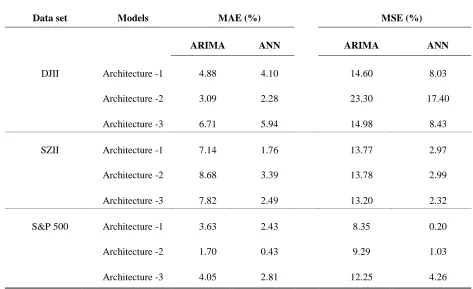
Table 5. The percentage improvement of the hybrid models in comparison with ARIMA and ANN models
Data set Models MAE (%) MSE (%)
ARIMA ANN ARIMA ANN
DJII Architecture -1 4.88 4.10 14.60 8.03
Architecture -2 3.09 2.28 23.30 17.40
Architecture -3 6.71 5.94 14.98 8.43
SZII Architecture -1 7.14 1.76 13.77 2.97
Architecture -2 8.68 3.39 13.78 2.99
Architecture -3 7.82 2.49 13.20 2.32
S&P 500 Architecture -1 3.63 2.43 8.35 0.20
Architecture -2 1.70 0.43 9.29 1.03
7. Conclusion
Time series forecasting has drawn overwhelming attention in variety areas, especially financial markets. Forecasting accuracy is one of the most important factors in choosing a right forecasting model and play a main role in many decision making processes. Despite numerous individual models available in the literature of time series forecasting, accurate forecasting is still one of the most challenging issues facing decision makers and investors. It is demonstrated in the literature that combining different models is an effective strategy to generate superior results in comparison with individual models and improve accuracy of forecasting.
In this paper, three combination architectures of ARIMA and ANN models, which are the most important and widely used linear and nonlinear forecasting models; respectively, are presented in order to improve forecasting accuracy, overcome the drawbacks of ARIMA and ANN models, and obtain forecasting results in financial markets that are more reliable. Empirical results with three benchmark data sets, elected from international stock markets, including Dow Jones Industrial Average Index (DJIAI),Shenzhen Integrated Index (SZII) and standard and poor’s (S&P 500) indicate that all aforementioned hybrid models produce outstanding results than their components. The average improvements yielded over than ARIMA and ANN models in terms of MSE in the test data set for DJIAI are 17. 63% and 11.29%, for SZII are 13.58% and 2.76% and for S&P500 are 9.96% and 1.83%, respectively. Thus, combining different models is an effective way in order to obtain more accurate results for financial time series forecasting.
Future research can aim at combining other forecasting tools, like SVM and GARCH models, in evaluating the ability of the proposed hybrid models. Besides, for situations under incomplete data conditions, fuzzy forecasting methods can be used in order to construct hybrid architectures. Another direction is to examine more weighting approaches such as genetic or differential evolutionary (DE) algorithms to find optimum weights in architecture combination-3. The future work also involves extending three combination architectures for three or more individual models. Besides, the proposed hybrid models can be tested in different areas such as engineering sciences for producing more accurate forecasting results.
Reference
Aladag, C., Egrioglu, E and Kadilar,C., 2009“ Forecasting nonlinear time series with a hybrid methodology”, Applied Mathematics Lettres, Vol.22, PP.1467-1470.
Areekul, P., Senjyu, T., Toyama, H and Yona, A.,2010, “Notice of violation of IEEE publication principles a hybrid ARIMA and neural network model for short-term price forecasting in deregulated market”, IEEE Transactions on Power Systems, Vol.25 ,PP.524-530.
Babu, C.Narendra.,Reddy, B.Eswara.,2012 “A moving- average filter based hybrid ARIMA-ANN model for forecasting time series data”, Applied Soft Computing, Vol.27, PP.27-38.
Bates, J.M., Granger, C.W.J., 1969, “The combination of forecasts”, Journal of the Operational Research Society, Vol.20, No.4, PP.46-451.
Box ,P., Jenkins, G.M.,1976, Time Series Analysis: Forecasting and Control, Holden-day Inc., San Francisco, CA.
Ebrahimpour, R., Nikoo,H.,Masoudnia,S., Yousefi,M.R and Ghaemi, M.S., 2011, “Mixture of MLP-experts for trend forecasting of time series: A case study of the Tehran stock exchange”, International Journal of Forecasting,Vol. 27, No.3, PP.804-816.,
Gairaa, K.,Khallaf,A.,Messlem,Y and Chellali.,F.,2016 “Estimation of the daily global solar radiation based on Box–Jenkins and ANN models: A combined approach”, Renewable and Sustainable Energy Reviews, Vol.57, PP.238-248.
Katris, CH., Daskalaki, S., 2015, “Comparing forecasting approaches for Internet traffic”, Expert Systems with Applications, No. 42, PP. 8172–8183.
Khashei, M. Bijari, M.,2012, “Hybridization of the probabilistic neural networks with feed-forward neural networks for forecastin”, Computers & Industrial Engineering, PP.1277-1288.
Khashei, M., Bijari, M., 2011 “A novel hybridization of artificial neural networks and ARIMA models for time series forecasting”, Applied Soft Computing, Vol.11, PP.2664–2675.
Khashei, M., Bijari, M.,2010, “An artificial neural network (p, d ,q) model for timeseries forecasting”, Expert Systems with Applications,Vol. 37, PP.479–489.
Khashei, M., Hejazi, S.R and Bijari, M.,2008, “A new hybrid artificial neural networks and fuzzy regression model for time series forecasting”,Fuzzy Sets and Systems, Vol.159, No.7, PP.769-786.
Kristjanpoller, W., M.C. Minutolo.,2015, “Gold price volatility: A forecasting approach using the Artificial Neural Network–GARCH model”, Expert Systems with Applications,Vol.42, No.20, PP.7245-7251.
Kumar, M., Thenmozhi, M.,2014, “Forecasting stock index returns using ARIMA-SVM, ARIMA-ANN, and ARIMA-random forest hybrid models”, International Journal of Banking, Accounting and Finance, Vol.5, No.3, PP.284-300.
Moeeni, H., Bonakdari, H., 2016, “Forecasting monthly inflow with extreme seasonal variation using the hybrid SARIMA-ANN model”, Stoch Environ Res Risk Assess.
Pai, P-F., W-C, Hong. 2005, “Support vector machines with simulated annealing algorithms in electricity load forecasting”, EnergyConversion and Management, Vol.46, No.17, PP.2669-2688.
Pham, H.T., Yang, B.-S., 2010 “Estimation and forecasting of machine health condition using ARMA/GARCH model”, Mechanical Systems and Signal Processing, Vol.24, No.2, PP.546-558.
Reid, D.J., 1968, combining three estimates of gross domestic product, Economica, PP.431-444.
Shafie-khah, M., Moghaddam, M. P. and Sheikh-El-Eslami, M. K.,2011, “Price forecasting of day-ahead electricity markets using a hybrid forecast method”, Energy Conversion and Management,Vol.52, PP.2165-2169.
Wang, J.-J., Wang,J-Z., Zhang,Z-G and Guo, SH-P., 2012, “Stock index forecasting based on a hybrid model”, Omega, Vol.40, No.6, PP.766-758.
Wongsathan, R., Seedadan, I., 2016, “A hybrid ARIMA and Neural Networks model for PM-10 pollution estimation: The case of Chiang Mai city moat area”,Procedia Computer Science, No, PP. 86 273 – 276. Xiong,T., Li,Ch and Bao., Y., 2017, “Interval-valuedtimeseriesforecastingusinganovelhybrid HoltI and MSVR model”, Economic Modelling, Vol. 60, PP. 11–23.
Yuan, X., Tan, Q., Lei, X., Yuan, Y., and Wu , X.,2017, “Wind power prediction using hybrid autoregressive fractionally integrated moving average and least square support vector machine”, Energy, NO.129, PP. 122-137.