A review on low‑dimensional physics‑based
models of systemic arteries: application
to estimation of central aortic pressure
Shuran Zhou
1, Lisheng Xu
1,2*, Liling Hao
1, Hanguang Xiao
3, Yang Yao
1, Lin Qi
1and Yudong Yao
1,2Introduction
Cardiovascular diseases have become a dominant factor of mortality all over the world [1]. Nearly 17.5 million people die of cardiovascular disease [2] and billions of dollars are spent every year on related healthcare [3]. Nowadays, cardiovascular research has become an important topic and been paid significant attention by researchers. Cardi-ovascular system is a complex circulatory system consisting of the heart, arteries and veins [4]. In recent years, due to the significant improvements in computer technol-ogy, modeling based on physical principles has become a powerful tool to simulate the
Abstract
The physiological processes and mechanisms of an arterial system are complex and subtle. Physics-based models have been proven to be a very useful tool to simulate actual physiological behavior of the arteries. The current physics-based models include high-dimensional models (2D and 3D models) and low-dimensional models (0D, 1D and tube-load models). High-dimensional models can describe the local hemody-namic information of arteries in detail. With regard to an exact model of the whole arterial system, a high-dimensional model is computationally impracticable since the complex geometry, viscosity or elastic properties and complex vectorial output need to be provided. For low-dimensional models, the structure, centerline and viscosity or elastic properties only need to be provided. Therefore, low-dimensional modeling with lower computational costs might be a more applicable approach to represent hemo-dynamic properties of the entire arterial system and these three types of low-dimen-sional models have been extensively used in the study of cardiovascular dynamics. In recent decades, application of physics-based models to estimate central aortic pressure has attracted increasing interest. However, to our best knowledge, there has been few review paper about reconstruction of central aortic pressure using these physics-based models. In this paper, three types of low-dimensional physical models (0D, 1D and tube-load models) of systemic arteries are reviewed, the application of three types of models on estimation of central aortic pressure is taken as an example to discuss their advantages and disadvantages, and the proper choice of models for specific researches and applications are advised.
Keywords: Physics-based model, Systemic arteries, Central aortic pressure, 0D model, 1D model, Tube-load model
Open Access
© The Author(s) 2019. This article is distributed under the terms of the Creative Commons Attribution 4.0 International License (http://creat iveco mmons .org/licen ses/by/4.0/), which permits unrestricted use, distribution, and reproduction in any medium, provided you give appropriate credit to the original author(s) and the source, provide a link to the Creative Commons license, and indicate if changes were made. The Creative Commons Public Domain Dedication waiver (http://creat iveco mmons .org/publi cdoma in/zero/1.0/) applies to the data made available in this article, unless otherwise stated.
REVIEW
*Correspondence: [email protected] 1 Sino-Dutch Biomedical and Information Engineering School, Northeastern University, Shenyang 110819, China
hemodynamic properties of cardiovascular system and has been playing an increasingly important role in the diagnosis of cardiovascular diseases and the development of medi-cal devices [5–7].
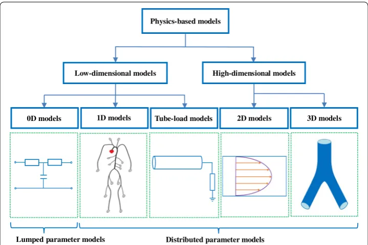
Current physics-based models can be divided into two categories, high-dimensional
models and low-dimensional models as shown in Fig. 1. High-dimensional models
including 2D models and 3D models can give detailed descriptions of the local flow field of the blood. These models describe the complex hemodynamic phenomenon of a specific region in the cardiovascular system. 2D models are generally used to describe changes of the radial blood flow velocity in an axisymmetric tube [8, 9]. 3D models are usually applied to simulate the fluid-structure interaction between the vascular walls and blood [10, 11]. To establish a 3D model of the entire arterial tree, the complex geometri-cal and mechanigeometri-cal information needs to be provided, which results in the enormous computational complexity, so that it cannot be readily implemented in practice. Conse-quently, high dimensional models can generally be used to simulate local hemodynamics of specific arterial sites, instead of the whole arterial tree.
In contrast to high-dimensional models, low-dimensional models with small computa-tional costs can readily reproduce the pulse wave propagation phenomenon and realize patient-specific modeling. Thus, the low-dimensional modeling can be an effective way to describe the hemodynamic properties of the entire arterial tree in practical applica-tions. At present, the available low-dimensional models mainly consist of 0D models, 1D models and tube-load models. 0D models, also called lumped parameter models, can describe global properties of the arterial system. The lumped parameter models are characterized by their pulse waveforms as a function of time only. The most well-known lumped parameter model is the Windkessel model [12], which includes mono-compart-ment models and multi-compartmono-compart-ment models [13, 14]. 1D models and tube-load mod-els are distributed parameter modmod-els, which can represent distributed properties of the
3D models 2D models
Lumped parameter models Distributed parameter models High-dimensional models Low-dimensional models
Physics-based models
0D models 1D models Tube-load models
arterial system. In the latter two types of models, their pulse waveforms depend on both time and space. In the distributed parameter models, 1D model based on the simpli-fied Navier–Stokes equation is commonly used to reproduce pressure and flow at any position in the entire arterial tree [15–19]. The Windkessel model is computationally simple but less accurate. On the other hand, 1D model can represent the wave propaga-tion phenomenon accurately but need a relatively large amount of computapropaga-tion. Tak-ing advantage of both Windkessel models (simplicity) and 1D models (accuracy), some researchers developed tube-load models [20, 21]. Tube-load models can monitor mul-tiple arterial hemodynamic parameters such as pulse transit time, arterial compliance, pulse wave velocity, and so on.
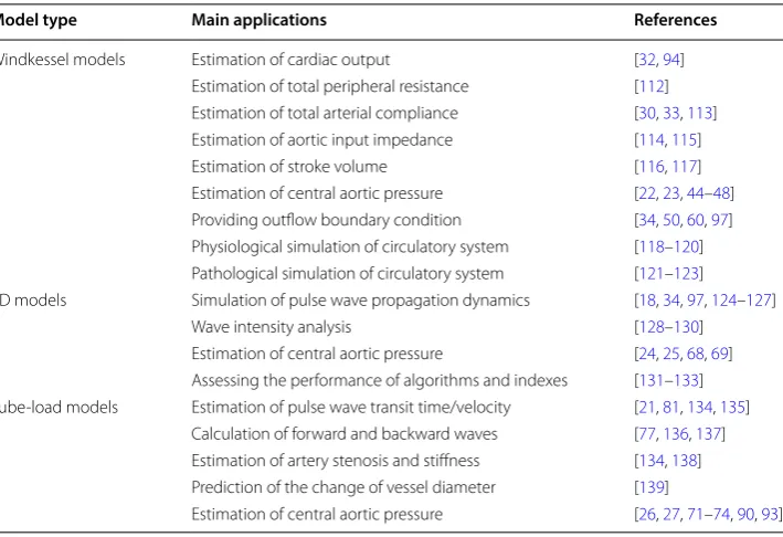
So far, these three types of low-dimensional models have been extensively used in the study of cardiovascular dynamics as shown in Table 1. Especially, applying phys-ics-based models to estimate central aortic pressure has been paid much attention in recent decades [22–27]. However, to our best knowledge, there has been few review paper about the reconstruction of central aortic pressure using these physics-based models. Additionally, estimating central aortic pressure is a common application of these three types of models, which contributes to compare their advantages and dis-advantages fully. Thus, this paper is to review three types of low-dimensional physics-based models (0D models, 1D models and tube-load models) of the arterial system and take the application of estimating central aortic pressure as an example to com-pare their advantages and disadvantages. To begin with, the theories and applications of Windkessel models including mono-compartment and multi-compartment models are described. Then, the theories and applications of two types of distributed parame-ter models, namely 1D models and tube-load models, are elaborated. Next, the advan-tages and disadvanadvan-tages of these three models are discussed. Finally, future challenges and final conclusion are presented.
Table 1 Main applications of Windkessel models, 1D models and tube-load models
Model type Main applications References
Windkessel models Estimation of cardiac output [32, 94]
Estimation of total peripheral resistance [112]
Estimation of total arterial compliance [30, 33, 113]
Estimation of aortic input impedance [114, 115]
Estimation of stroke volume [116, 117]
Estimation of central aortic pressure [22, 23, 44–48] Providing outflow boundary condition [34, 50, 60, 97] Physiological simulation of circulatory system [118–120] Pathological simulation of circulatory system [121–123] 1D models Simulation of pulse wave propagation dynamics [18, 34, 97, 124–127]
Wave intensity analysis [128–130]
Estimation of central aortic pressure [24, 25, 68, 69] Assessing the performance of algorithms and indexes [131–133] Tube-load models Estimation of pulse wave transit time/velocity [21, 81, 134, 135]
Calculation of forward and backward waves [77, 136, 137] Estimation of artery stenosis and stiffness [134, 138]
Prediction of the change of vessel diameter [139]
0D models
In 0D models (lumped parameter models), the Windkessel theory is applied to the modeling of the arterial system [12, 28, 29]. Windkessel models are divided into two classes: mono-compartment models and multi-compartment models. Theories and applications of two categories of models are elaborated in this part, respectively. Fur-thermore, the comparison of different Windkessel models is made in Table 2.
Model descriptions Mono‑compartment models
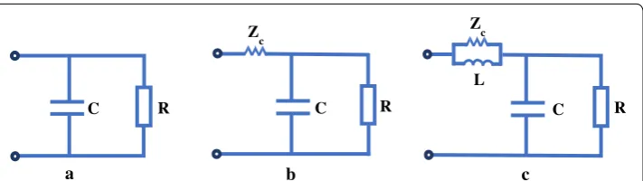
The mono-compartment model is a combination of inductance, compliance and resistance. According to the number of elements included, current mono-compart-ment models are classified into four main types: two-elemono-compart-ment, three-elemono-compart-ment, four-element and complex mono-compartment Windkessel models.
a. Two‑element Windkessel model The two-element Windkessel model is the simplest
mono-compartment model presented by Frank [12], which is made up of a resistor
(R) and a capacitor (C) as shown in Fig. 2a. In this model, the resistor describes the resistance of small peripheral vessels and the capacitor describes the distensibility of large arteries. The two-element Windkessel model simply describes the pressure decay of the aorta in diastole. This model cannot signify the high frequency effects because there is merely a time constant in the model. Owing to its simplicity, this model can be
Table 2 Comparison of different Windkessel models
Model type Mono-compartment model Multi-compartment
model Two-element model Three-element
model Four-element model
Strengths The model structure is
simplest The model can describe high fre-quency effects
The model can represent all the fre-quency effects well
The model can rep-resent pulse wave propagation Weaknesses The model cannot
represent high frequency effects
There is small error at
low frequency Parameter estimation is difficult The model structure is more intricate
The model cannot describe pulse wave propagation
a
C L
c
R Zc
R C
b Zc
R C
used in clinical practice readily such as total arterial compliance estimation [30] and blood pressure estimation [31].
b. Three‑element Windkessel model Adding a characteristic impedance ( Zc ) to the
two-element Windkessel model, the three-element Windkessel model is formed as shown in Fig. 2b [15]. The characteristic impedance is equal to oscillatory pressure divided by oscillatory flow. Although it is found that a resistance numerically equals approximately a characteristic impedance, the characteristic impedance is different from the resistance. The characteristic impedance is merely used to signify oscillatory phenomena. Owing to the inclusion of the characteristic impedance, this model can simulate high frequency effects. Simultaneously, the introduction of the characteristic impedance also results in some errors at the low frequency. In contrast with the two-element Windkessel model, the three-two-element Windkessel model can have a higher accuracy. Therefore, the three-element Windkessel model has been extensively used in theoretical research [32–34].
c. Four‑element Windkessel model Taking the inertance of blood flow into consideration on the basis of the three-element Windkessel model, Stergiopulos et al. [35] proposed a four-element Windkessel model as shown in Fig. 2c. Due to the addition of the inertance, this model can represent middle frequency effects. In other words, the four-element Windkessel model can simulate all frequency effects. It has been validated that the four-element model can give a better description of the impedance characteristics [36]. Some nonlinear regression analysis methods are applied to the estimation of the four-element model parameters. Compared with the two-element and three-element Windkessel mod-els, it is more difficult to identify the model parameters of the four-element Windkessel model. Consequently, only a few researchers make use of this model [23, 37, 38].
d. Complex mono‑compartment models For the sake of the further improvement of the arterial model, a few researchers developed more complex Windkessel models in which more resistive, inductive and capacitive components were introduced [39, 40]. By including more resistive and inductive elements, the laminar oscillatory flow impedance can be simulated. Owing to the high complexity of these models, there has been no further development by other investigators.
Multi‑compartment models
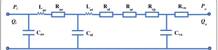
Regardless of spatial information, the mono-compartment model regards all arteries as a single block. In order to represent the distribution of flow and pressure, some multi-compartment models which were composed of a series of mono-multi-compartment mod-els were established. Figure 3 is an example of a simple multi-compartment model of the systemic arteries [42]. Every mono-compartment model is a combination of resist-ance (R), inertresist-ance (L) and compliresist-ance (C). At present, there are four typical compart-mental configurations in the multi-compartment model: T, and inverted L element,
respectively [13]. The corresponding compartmental configuration should be chosen appropriately according to the characteristics of the particular arteries. Since the multi-compartment model represents position information roughly but in general does not signify the nonlinear convective acceleration term of 1D model, this model is usually seen as the first order discretization of the one-dimensional linear model [43].
Applications
Mono-compartment models are simplified descriptions of an arterial system, simulating physiological properties of the arterial vessels with a few parameters. Multi-compart-ment models construct a full arterial network by connecting several mono-compart-ment models, describing particular information of different vessel compartmono-compart-ments. Due to the simplicity of mono-compartment and multi-compartment models, merely a few researchers used them to reconstruct central aortic pressure.
In Windkessel models, proximal flow or peripheral pressure measurements were fre-quently used as inflow condition. Many researchers chose aortic flow as model input [22, 44, 45]. Flow at other positions was selected as model input, such as carotid flow [46], left ventricle flow [23] and mitral valve mean flow [47]. Few researchers chose brachial and radial pressure as model input [48]. For model parameter acquisition, the majority of researchers calculated model parameters by population averaging [22, 23, 44–46, 48] and only a small number of researchers adopted partially individualized model param-eters [47].
Mono-compartment models are more commonly applied to the estimation of central aortic pressure than multi-compartment models. For example, the pressure waveform in the aorta was reconstructed by Stergiopulos et al. [44] and Struijk et al. [45] using a two-element Windkessel model. Cai et al. [22], Zala et al. [46] and Vennin et al. [22] employed a three-element Windkessel model to calculate central aortic pressure. A four-element Windkessel model was adopted by Her et al. [23] to reproduce the patient’s
Pi Po
Cao
Rvn
Cvn Cat
Lao
Qi Qo
Lat Rat Rar Rcp Rao
aortic pressure waveform undergoing counter-pulsation control by ventricular assist devices. Revie et al. [47] used a six-chamber lumped parameter model consisting of left ventricle and right ventricle, aorta, pulmonary artery, pulmonary vena cava and pul-monary vein to monitor aortic pressure changes. It was verified in clinical data [22, 23, 47] that Windkessel models can describe the general shape of pressure waveform in the ascending aorta, however, it is difficult to show the details of pressure waveform such as dicrotic notch features. Therefore, Windkessel models have limited accuracy for the esti-mation of central aortic pressure.
1D models
1D models are distributed parameter models. Theory and application of 1D models are described in this part, respectively. 1D models mainly focus on methods that solve one-dimensional equations and boundary conditions (including inflow, bifurcation and out-flow conditions).
Model descriptions Model derivations
The one-dimensional arterial flow theory was proposed by some researchers [16, 17]. Euler [49] first established a 1D model using the one-dimensional theory. Although assumptions of the model are simple, it laid foundations for further studies. Reymond et al. [50] extended the existing 1D model to a more detailed model consisting of the foot and hand circulation. Moreover, the ventricular-arterial coupling model was developed and 1D model of the circulation was validated. 1D models are commonly used to rep-resent pulse wave propagation phenomena of large arteries [29]. In the 1D model, the blood is assumed to be an incompressible Newton fluid and the vessel is an axisymmet-ric cylindaxisymmet-rical tube. The 1D model is governed by two equations [51]. A continuity equa-tion (see Eq. 1) and a momentum equation (see Eq. 2) both together describe the motion of the blood flow and the vessel wall. The formulas are as follows
where x is the distance along the vessel, t is time, q is the blood flow rate, p is the blood pressure, A is the cross-sectional area, r is the vessel radius, ρ is the blood density and µ is the viscosity.
Solving methods
For solving 1D Navier–Stokes equations, there are two types of methods including time domain and frequency domain methods. The time domain method can solve linear or nonlinear equations and frequency domain method can only solve linear equations.
a. Time domain method Generally, Navier–Stokes equations of 1D models are nonlin-ear, which are solved in the time domain using numerical methods. At present, there are
(1)
∂q
∂x+
∂A
∂t =0.
(2)
∂q
∂t +
4
3 ∂qA2
∂x = − A
ρ ∂p
∂x−
8µ
many numerical methods for solving the partial differential equations. Each method has its scope of application. The method of characteristics, finite difference method, finite volume method, finite element method and spectral method are frequently used to solve 1D pulse propagation equations.
The method of characteristics is a basic method of solving the partial differential equa-tions. The essence of this method is the integral along the characteristic line of the par-tial differenpar-tial equations to simplify the form of equations. The characteristic method has a clear physical meaning and a wide application scope. As for solving the differential equations of three independent variables, the method of characteristic can be very com-plicated, and there are still some problems to be solved. The governing equations can be solved by taking use of the method of characteristics [52–54].
The finite difference method is a numerical method for solving complex partial differ-ential equations by approximating the derivatives with finite differences. While the prin-ciple of the finite difference method is simple, it can give the corresponding difference equation for any complex partial differential equation. Difference equations can only be considered as mathematical approximations of differential equations. This method has been used by a number of researchers. For instance, Olufsen et al. applied the two-step Lax–Wendroff method to solving the continuity and momentum equations [18, 19].
A finite volume method is developed on the basis of the finite difference method. To begin with, the calculated region is divided into a series of control volumes and there is a control volume at the surrounding of each grid point. Then each control volume is integrated and a set of discrete equations are obtained. Finally, the discrete equations need to be solved. The finite volume method is suitable for the computation of fluid. This method has a high computing speed and low requirements for the grid, but its precision is limited. To solve the differential equations, the finite volume method is often used [55, 56].
The finite element method uses the variational principle to minimize the error func-tion. The advantage of the finite element method is that this method can simulate complex curve or surface boundary accurately. Furthermore, the division of the grid is arbitrary and it can design the general program easily. Nevertheless, the finite element method cannot give a reasonable physical explanation and some errors in the calculation are still difficult to improve. Recently, some investigators used the finite element method to solve the differential equations [57–59].
The spectral method is a class of computing techniques of using an orthogonal func-tion or intrinsic funcfunc-tion as an approximate funcfunc-tion to solve certain differential equa-tions. The superiorities of the spectral method are to obtain a higher precision using fewer grid points. The poor stability and high complexity in the treatment of boundary conditions are the major weaknesses of this method. The spectral method has been uti-lized to solve the one-dimensional pulse wave propagation equations by a few research-ers [60, 61].
propagation theory, linear 1D Navier–Stokes equations (see Eqs. 3, 4) in hemodynamics are converted into electrical transmission line equations (see Eqs. 5, 6) in the circuit [62]. The subsequent work is that we can employ methods of solving electric circuit to solve 1D Navier–Stokes equations. A transmission line equivalent circuit of an arterial segment is represented as shown in Fig. 4.
where U is the voltage, I is the current, R= πr8µ4 is the resistance, L= ρ A=
ρ
πr2 is the inductance, C= dAdp = 32πEhr2 is the capacitance, E is the Young’s modulus, and h is the arterial wall thickness. G is the conductance, describing blood flow leakage, which is usually neglected. The electrical circuit is comprised of resistive, inductive and capaci-tive elements. The values of these elements are calculated from mechanical and geomet-ric parameters in the arterial tree.
Boundary conditions
For 1D pulse wave propagation equations, boundary conditions, commonly including inflow, bifurcation and outflow boundary conditions, need to be determined.
a. Inflow conditions The flow waveform measured in vivo at ascending aorta or aortic root serves as the inflow condition using a magnetic resonance imaging or ultrasound equip-ment. Alternatively, a flow function derived from a simple model of the heart can serve as the inflow condition. The function is periodic which is mainly determined by the cardiac period and the cardiac output parameters [18].
(3)
−∂q ∂x =
dA dp
∂p ∂t =0.
(4)
−∂p∂x = ρA∂q∂t + πr8µ2q.
(5)
−∂I
∂x = UG+C
∂U ∂t .
(6)
−∂∂Ux = IR+L∂I
∂t.
(7)
q(0,t)= CO t τ2e
−t2
2τ2, 0≤t<T.
a
C L
R
Z input
b G
Source Transmission line Load
Zc
ZL
where CO denotes the cardiac output, τ denotes the time for cardiac output to reach its maximum and T denotes the cardiac period.
The other inflow condition is that the left ventricle of the heart is coupled to 1D arterial tree model. Two main heart models are developed to represent the rela-tionship between the ventricular pressure and volume. The time-varying elastance model is that the heart is seen as an elastance varying with time [63]. This left ven-tricular model indicates the instantaneous change of pressure and volume in left ventricle.
where E is the elastance, P is the instantaneous pressure of left ventricle, V is the instan-taneous volume of left ventricle and V0 is the volume intercept of the end-systolic line.
The one-fiber model is another heart model in which the heart is described as a rotationally-symmetric cylindrical or spherical cavity [64]. The left-ventricular pump function is reflected by wall tissue function. It is assumed that fiber stress and strain are homogeneously distributed in the thick wall. The ratio of the fiber stress ( τf ) to the pressure of the left ventricle ( Plv ) is closely related to the ratio of the wall volume ( Vw ) and the cavity volume ( Vlv).
b. Bifurcation conditions In arterial networks, vessel branching is another impor-tant sort of boundary condition. At the bifurcation, the principle of pressure and flow continuity was applied [32, 55, 59, 65]. It is assumed that all bifurcations are situated at a point and the effect of the bifurcation angles is ignored. Without any blood leak-age, according to the conservation of mass, the outlet flow of a parent vessel is equal to the sum of the inlet flow of two daughter vessels at the bifurcation (see Eq. 11). Considering the continuity of pressure, the pressure of a parent vessel and the pres-sure of each daughter vessel are identical at the bifurcation (see Eq. 12). In reality, there exist energy losses at the bifurcations. Generally, the energy loss at a bifurcation is quite small and they are often neglected. For the bifurcation at the aortic arch, how-ever, large energy losses are brought about. Because it has a nearly right-angled turn and a high velocity of blood at this bifurcation, remarkable vortices are produced. In order to represent the loss at the aortic arch bifurcation, a loss coefficient K is intro-duced [19] (see Eq. 13).
where u¯x denotes the average axial velocity and ρ denotes the density. The subscripts pa and d indicate the parent and the daughter vessel, respectively.
(8)
q(0,t+jT)= q(0,t), j=1, 2, 3,. . .
(9)
E(t)= P(t) V(t)−V0
.
(10)
Plv τf =
1 3ln
1+ Vw
Vlv
.
(11)
qpa= qd1+qd2.
(12) ppa= pd1=pd2.
(13) pdi= ppa+
ρ 2((u¯x)
2
pa−(u¯x)2di)−
Kdi 2 (u¯x)
2
c. Outflow conditions The simplest outflow boundary condition is that the terminal of vessel is seen as a pure resistive load [18]. Nevertheless, a precise peripheral resistance value is not easy to be determined. Assuming a constant relation between pressure and flow, pressure and flow are in phase, actually, which is not physiologically reasonable for large arteries. The pure resistance model is merely suitable for small arteries. To over-come the weaknesses, a phase-shift between pressure and flow should be applied to the downstream boundary. The terminal impedance for the pure resistance is as follows.
where ZL(w) denotes the terminal impedance of large arteries and RT denotes the peripheral resistance.
The distal network of truncated vessel is represented as the terminal impedance which is modeled by a three-element Windkessel model [66]. The three-element Windkessel model is made up of a resistance R1 in series with a parallel combination of a capacitor CT and another resistance R2 . This model cannot represent the wave propagation effects. The frequency dependent impedance of Windkessel model is given by
The relation between pressure and flow at the truncated arteries is given by the following differential equation.
In recent years, the structured-tree model presented by Olufsen [67] has become a pop-ular outflow boundary condition. Compared with the resistance and Windkessel model, the structured-tree model can simulate the impedances of small arteries more accu-rately. At the terminal branches of the truncated arterial tree, a structured-tree model, which is based on linear one-dimensional Navier–Stokes equations, provides a dynamic boundary condition for large arteries. The model can describe the phase lag between pressure and flow and the high frequency oscillations. Meanwhile, it can also represent the wave propagation effects of arterial system. According to the convolution theorem, the outflo w boundary condition is obtained by
The root impedance is computed from the relationship between pressure and flow as follow
where g =cC , c denotes the wave propagation velocity, ZL(w) denotes the root imped-ance, namely, the terminal impedance of large arteries, Z(L, w) denotes the terminal impedance of small arteries, L denotes the vessel length and w denotes the angular frequency.
(14) ZL(w)=RT
(15) ZL(w)=
R1+R2+iwCTR1R2
1+iwCTR2
.
(16) ∂p
∂t =R1 ∂q ∂t −
p
R2CT +
q(R1+R2)
R2CT
.
(17) p(x,t)= 1
T
T/2
−T/2
z(x,t−τ )q(x,τ )dτ.
(18)
ZL(w)=
ig−1
sin(wL/c)+Z(L,w)cos(wL/c)
Applications
1D models can simulate pressure and flow waveforms at any point of the arterial net-work according to their distributed properties. Since 1D models include too many vascular parameters, they haven’t been extensively used to reconstruct central aortic pressure up to now. By limiting the number of personalized parameters, 1D models may have a great potential for estimation of central aortic pressure in clinical practice.
For 1D models, aortic flow waveform is the most common inflow condition [24,
68]. Few researchers used peripheral pressure measurement (e.g. brachial pressure or radial pressure) as model input [25, 69]. The aortic flow waveform can be measured by ultrasound equipment, however, it is not accurate. Meanwhile, it is very expensive to obtain aortic flow waveforms by MRI equipment. The pressure waveforms of good stability can readily be recorded using peripheral pressure sensors such as applana-tion tonometry. Generally, vascular geometric parameters of 1D models are meas-ured by MRI or CT equipment, which is costly and complex. Many researchers used population averages for these geometric parameters. Nevertheless, Harana et al. [24] measured aortic geometry parameters including ascending aorta, descending aorta and three supra-aortic branches using MRI equipment. Meanwhile, pulse wave veloc-ity (PWV) and vascular resistance and compliance parameters for each subject were calculated from measured data. Remaining blood flow parameters such as density and viscosity were assumed to be constants.
In recent years, 1D models with different degrees of complexity have been utilized by several researchers to reconstruct central aortic pressure. For example, Bárdossy et al. [69] presented a “backward” calculation method to derive central aortic pressure waveform in a 1D model comprising 50-segment arteries. A personalized transfer function between aorta and radial was established by Jiang et al. [24] to estimate cen-tral aortic pressure based on 1D model including 55 large arteries and 28 small arter-ies. Khalifé et al. [68] estimated absolute pressure in the aorta by combining a reduced 1D model including an ascending aorta branch and a descending aorta branch with MRI. A non-invasive personalized estimation method of central aortic pressure was developed by Harana et al. [24] using a 1D aortic blood flow model. Owing to the complexity of 1D models, the details of pressure waveform can be described easily [24]. If all vascular geometric parameters are measured by noninvasive equipments, 1D models can provide accurate estimation of central aortic pressure.
Tube-load models
Tube-load models are distributed parameter models. Theory and application of tube-load models are described in this part, respectively. Tube-tube-load models mainly focus on various tube models based on different assumptions.
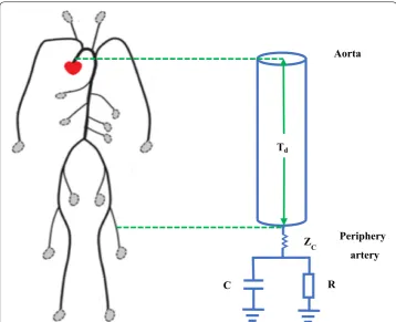
Model descriptions
and the load signifies the wave refection site in the arterial terminal. The formulas are as follows.
where L denotes the large artery inertance, C denotes the large artery compliance, d denotes length of tube, Td denotes the time delay, Zc denotes the characteristic imped-ance, ZL denotes the terminal impedance, Ŵ denotes the wave reflection coefficient, P (19) Td =
√ LC
(20) Zc=
L/C
(21)
Ŵ(jw)= ZL(jw)−Zc
ZL(jw)+Zc
(22) P(x,jw)= Pf(0,jw)ejwTdx/d+Pb(0,jw)e−jwTdx/d
(23) Q(x,jw)= 1
Zc(Pf(0,jw)e jwTdx/d
+Pb(0,jw)e−jwTdx/d)
(24) Pp(jw)=
jw+ RC1 +2Z1 cC
ejwTd+ 1
2ZcCe
−jwTd
jw+RC1 + Z1 cC
Pc(jw)
Periphery artery
R ZC
Aorta
C
Td
denotes the pressure, Q denotes the flow. In addition, the subscripts f, b, c and p are for the forward and backward wave, aorta and peripheral artery, respectively.
For tube-load models, there are three main types of loads, including pure resistance, generic pole-zero, three-element Windkessel models. The pure resistance load is a high simplification of small arterial vessels, accounting for the peripheral resistance [26, 71]. The greatest advantage of this kind of load is simplicity and its disadvantage is that there is a big difference from the real vascular structure. The generic pole-zero models as a ter-minal impedance can change the order of system flexibly [72]. However, the weakness of the model is that model parameters do not have physiological significance. The most fre-quently used load is the three-element Windkessel model, which consists of a character-istic impedance, a resistance and a compliance [73, 74]. Although the Windkessel model fails to provide the detailed anatomical and mechanical information of arterial network, it can describe the lumped properties of terminal arterial vessels well.
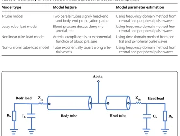
Based on different assumptions, tube-load models have been developed into T-tube, lossy tube-load, nonlinear tube-load and non-uniform tube-load models, which are summarized in Table 3. In comparison with the simplest tube-load model, these models have a higher accuracy in hemodynamic simulation.
T‑tube model
The T-tube model is a frequently-used tube-load model, in which there are two tubes with two terminal loads as shown in Fig. 6 [75, 76]. While the tubes signify head-end and body-end travel paths, the loads represent head-end and body-end reflection sites,
Table 3 Summary of tube-load models based on different assumptions
Model type Model feature Model parameter estimation
T-tube model Two parallel tubes signify head-end
and body-end propagation paths Using frequency domain method from central and peripheral pulse waves Lossy tube-load model Blood pressure decays along the
arterial tree Using frequency domain method from central and peripheral pulse waves Nonlinear tube-load model Arterial compliance is an exponential
function of blood pressure Using time domain method from cen-tral and peripheral pulse waves Non-uniform tube-load model Tube exponentially tapers along
arte-rial vessels Using frequency domain method from central and peripheral pulse waves
Aorta
Rh Ch Zch
Rb Cb
Zcb Head load
Body load
Body tube Head tube
respectively. The advantages of the T-tube model are that it is a simple model and that it can indicate main features of pressure and flow waveforms in the large blood vessels. However, it cannot represent the wave reflection intensely depending on frequency.
Lossy tube‑load model
Tube-load models mentioned above are based on lossless tube-load models. The lossless tube-load model is a kind of ideal and simple model. In some situations, ignoring the loss of tube can bring large errors [77–80]. For example, for reconstructing the central aortic pressure waveform from peripheral pressure waveforms, it is generally assumed that the mean pressure is same at any position. In fact, the blood pressure loss is large along the arterial tree in pathophysiologic conditions or postoperative period. In order to improve the accuracy of tube-load models, Abdollahzade et al. [20] proposed the lossy tube-load model of arterial tree in humans as shown in Fig. 7. Compared with lossless tube-load models, lossy tube-load models have smaller errors and larger efficacy.
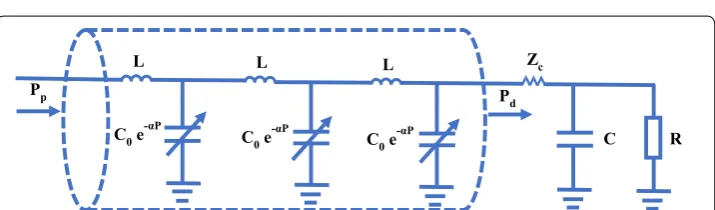
Nonlinear tube‑load model
Previously, tube-load models were regarded as linear models. In recent years, Gao et al. [81, 82] has developed a nonlinear tube-load model based on the exponential relation-ship between blood pressure and compliance as shown in Fig. 8. In the nonlinear tube-load model, arterial compliance is no longer a constant but a function of blood pressure.
R C
Zc
Pi Po
Pfi(t)
Pbi=e-γ(s)loPbo(t)
Pfo=e-γ(s)loPfi(t)
Pbo (t)
Aorta Periphery
Fig. 7 The lossy tube-load model. P the blood pressure, γ the wave propagation constant, l0 the length of the tube, R the peripheral resistance, C the load compliance, Zc the characteristic impedance; subscripts i and o are for the inlet and outlet of the tube, respectively
C0 e -αP
R C
C0 e-αP C0 e
-αP
Pd
Zc
L L L
Pp
In contrast with the linear tube-load model, the nonlinear tube-load model has a higher accuracy in estimating pulse transit time [21].
Non‑uniform tube‑load model
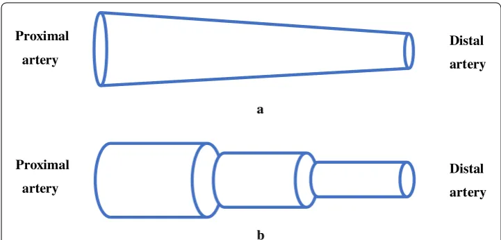
The electrical transmission line theory is applied to mathematical modeling of arterial vessels. It is generally assumed that the transmission line model is a uniform tube with a terminal load. Taylor [83] explored the wave propagation properties of a non-uniform transmission line, since the uniform tube is too simple to reflect the real characteristics of the arteries. Subsequently, Einav et al. [84] proposed an exponentially tapered trans-mission line model of the arterial system, in which the geometrical properties and wall elasticity of the tube exponentially tapered along the length of arterial vessels. At pre-sent, there are two methods to describe the taper effects of a non-uniform tube. One method is that the inductance and capacitance of the tube change with the position exponentially as shown in Fig. 9a [85–87]. Another method is that an artery is separated into several smaller segments and each segment is viewed as a uniform tube as shown in Fig. 9b [88, 89].
Applications
Tube-load models include tubes and loads, describing wave propagation and refection phenomenon with only a few parameters. Combining the advantages of Windkessel models (simplicity) and 1D models (accuracy), tube-load models have become an attrac-tive tool for the reconstruction of central aortic pressure waveform.
For tube-load models, inflow conditions are obtained from one or two measured peripheral pressure waveforms. A radial [71, 73, 74], brachial [26] or femoral [72] pres-sure meapres-surement is commonly used as model input. Moreover, some researchers [27, 90–92] chose two measured peripheral pressure waveforms as inflow conditions such as radial and femoral arteries. Because intravascular and extravascular pressure at radial artery is very close, the radial pressure waveform can be accurately recorded using an applanation tonometry. The brachial cuff-based measurement is a very convenient
b a Proximal
artery
Distal artery Proximal
artery
Distal artery
Fig. 9 The non-uniform tube-load model. a A non-uniform tube tapering with the position exponentially; b
approach for obtaining brachial pressure, especially suitable for longer term outpatient monitoring of central aortic pressure or potential general hospital ward usage.
Single tube or T-tube models with different loads are used to described the relation between central and peripheral pressures. For example, Swamy et al. [72] employed a single tube with a generic pole-zero load to establish an adaptive transfer function between aortic and femoral pressures. A single tube model with a resistance load was applied by Gao et al. [71] and Natarajan et al. [26] to the estimation of central aortic pressure. Individualized transfer functions were built by Sugimachi et al. [73] and Hahn et al. [74] using a single tube model with a three element Windkessel load. Ghasemi et al. [27, 90], Lee [91] and Kim et al. [92] utilized a T-tube model with a three-element Windkessel load, to reconstruct central aortic pressure from two measured peripheral pressure.
In order to acquire an adaptive or individualized transfer function, most researchers measured the pulse transit time for each subject through some noninvasive approaches and calculated the remaining parameters by population averaging [26, 27, 71–74, 92, 93]. Blind system identification is another method of estimating model parameters, which can reconstruct the central aortic pressure waveform from two distinct peripheral pres-sure waveforms [90, 91]. The blind system identification method can obtain fully indi-vidualized parameters. The weakness of this method is that it is inconvenient to measure multiple distinct peripheral pressure waveforms in clinical practice. To examine the performance of individualization, Hahn [93] made a comparative study on the estima-tion of central pressure among a fully individualized, two partially individualized and a fully generalized transfer functions based on tube-load models. The 9 swine experiment results showed that the fully individualized transfer function had higher accuracy than two partially individualized functions and the fully nonindividualized transfer function. Since in the tube-load model, only one parameter, the pulse transit time, could be readily individualized, tube-load models had moderate accuracy for estimation of central aortic pressure.
Discussions and conclusions Comparisons of three types of models
In this paper, recent progresses of Windkessel, 1D and tube-load models in the arterial system are reviewed. Windkessel models are developed into increasingly complicated and detailed structures and a variety of Windkessel models are established [39, 94]. 1D models including more arterial segments and coupling the heart have been set up in recent years [29, 50]. Tube-load models with various types of tubes based on different assumptions are investigated [77, 81, 83].
by a set of ordinary differential equations, this model is simpler than the distributed parameter model built by a set of partial differential equations. The model is fit for calcu-lating hemodynamic parameters and simucalcu-lating the whole circulatory system.
1D models and tube-load models are distributed parameter models which signify the distributed properties along the arterial vessels. 1D models can accurately predict flow and pressure in the entire arterial tree and the model parameters can truly reflect the physiological properties of arterial vessels [49]. A 1D model is determined by a set of partial differential equations with a lot of parameters. It is very difficult to determine a large number of parameters using system identification methods. The majority of geo-metrical and mechanical parameters can be directly measured by MRI, CT or Doppler ultrasound equipment. The rest of the parameters are approximated or seen as constants such as the thickness of arterial wall and width of boundary layer. The 1D model is an appropriate approach to study pulse wave propagation phenomenon in arterial system.
Tube-load models are a parallel connection of multiple tubes with parametric loads, which is a simplified 1D model. The tube indicates the path of pulse wave propagation and the load indicates the effective reflection point [75, 76]. The transit time of pressure and flow waves is described by the time delay constant parameter of the model. Tube-load models can represent the relationship between central and peripheral arteries with a few parameters. Once proximal and distal waveforms of the arterial tree are obtained, the parameters of tube-load models can be determined by system identification tech-niques. In comparison with 1D model, tube-load model has a lower computation cost. Meanwhile, the shortage of the tube-load model is that it is less accurate than 1D model. Tube-load models are suitable for investigating wave propagation and reflection.
Future challenges
Although a variety of physics-based models have been developed, there still exist a number of challenging problems to be solved. Multi-scale modeling, coupling of vari-ous systems and patient-specific modeling are very significant research subjects at present.
Multi‑scale modeling
A model of each scale has its scope of application [29, 97, 98]. Low-dimensional mod-els have low computational cost but poor accuracy, which is applicable to represent the global properties of the arterial networks. Nevertheless, high-dimensional models can offer high accuracy simulation but with greater complexity. They are commonly used to describe the local properties of arterial vessels in detail. Therefore, coupling models of various different scales can combine the advantages of different dimen-sional models [43, 99, 100]. Multi-scale modeling of arterial vessels can be a powerful tool for providing potential applications in clinical practice.
Coupling of various systems
There exist a variety of biological systems such as the nervous system and the respira-tory system in human body which run simultaneously and interactively. The effects of other biological systems are usually ignored in physical modeling of cardiovascular system. As a matter of fact, the nervous system has a significant impact on cardio-vascular system [101]. For example, as the blood pressure changes, to avoid dysfunc-tions, the sympathetic nerves and the parasympathetic nerves are usually motivated
Table 4 Comparison of Windkessel, 1D and tube-load models
Model type Windkessel models 1D models Tube-load models
Model structure Including capacitors,
resis-tors and inductance Dividing the arterial tree into many small seg-ments
Consisting of multiple tubes with terminal loads
Model parameters Few A lot Few
Easy to estimate Difficult to estimate Easy to estimate
Complexity Low High Moderate
Accuracy Low High Moderate
Simulate wave propaga-tion and reflecpropaga-tion phenomenon
No Yes Yes
Inflow condition Aortic flow function Aortic flow or pressure
waveforms Aortic pressure waveforms
Aortic pressure waveforms Aortic flow function Heart model
Outflow condition Venous pressure Pure resistance Windkessel model
Windkessel model Generic pole-zero model
Structured-tree model Pressure Pressure
Geometrical and
mechani-cal properties None Vessel diameter, length, thickness, elasticity and blood viscosity
to regulate cardiovascular response [101]. Smith et al. [102] proposed a modified cardiovascular model by including a minimal autonomic nervous system activation model. This modified model can simulate various cardiovascular diseases such as hypovolemic shock septic shock, cardiogenic shock, pericardial tamponade and pul-monary embolism.
Due to the fact that both the respiratory system and the cardiovascular system located in the thoracic cavity, the cardiovascular system can be influenced by the respiratory system strongly [103]. For example, an integrated model of the cardiopulmonary sys-tem was present by Albanese et al. [104], which included cardiovascular circulation, respiratory mechanics, gas exchange and neural control mechanisms. The physiological parameters in normal and pathological conditions were simulated and the interactions between the cardiovascular and respiratory systems were explained. Trenhago et al. [105] proposed a refined coupled model of the cardiovascular and respiratory systems, consisting of 19 compartments, in which the respiratory system was extended to include a complex system for gas exchange and transport. The advantage of the refined model is that it enables to simulate situations in which existing models cannot predict mimic and it helps us to understand complex mechanisms better. For modeling of cardiovascular system, the respiratory effects should be considered. In comparison with previous car-diovascular model, a modified carcar-diovascular model integrating neurological and res-piratory components has better accuracy. Hence, combining the nervous system and the respiratory system with the cardiovascular system might be a good way to improve the accuracy of models.
Patient‑specific modeling
Patient-specific models can provide opportunities for improving accuracy [106–108]. The patient-specific parameters can be obtained from imaging techniques such as mag-netic resonance imaging, computed tomography and ultrasound. A properly personal-ized model can predict physiological or pathological status more accurately [109, 110]. The personalized modeling in the arterial system can play an increasingly key role in the development of medical instruments.
have too many parameters, it is actually impossible to measure all parameters, however, human body size parameters are available easily. A statistical analysis has shown that the blood vessel sizes have close correlation with sex, age, height, and weight of a subject [111]. Furthermore, Young’s modulus representing vascular stiffness has a strong cor-relation with age. It might be possible to build cor-relationships between geometrical and mechanical parameters of 1D models and body size parameters of the subject. The geo-metrical and mechanical parameters can be firstly employed by population averages and then the average parameters can be calibrated with body size parameters. Combining with the two methods above, a modified 1D model may be the best choice for estimating central aortic pressure.
Conclusion
In conclusion, different physics-based models in cardiovascular system have differ-ent traits and the selection of models mainly depends on the aim of modeling includ-ing complexity and accuracy required. By discussinclud-ing the advantages and disadvantages of various physics-based models, this review contributes to a better understanding of physiological mechanism in the arterial system and provides effective guidance on low-dimensional physics-based modeling.
Authors’ contributions
SZ performed the literature review and drafted the manuscript; LX conceived the study and provided the theory of mathematical modeling; LH, HX and YaY checked the manuscript; LQ and YuY gave suggestions and revised the manu-script. All authors read and approved the final manumanu-script.
Author details
1 Sino-Dutch Biomedical and Information Engineering School, Northeastern University, Shenyang 110819, China. 2 Neusoft Research of Intelligent Healthcare Technology, Co. Ltd., Shenyang 110167, China. 3 Chongqing Key Labora-tory of Modern Photoelectric Detection Technology and Instrument, School of Optoelectronic Information, Chongqing University of Technology, Chongqing 400054, China.
Competing interests
The authors declare that they have no competing interests. Availability of data and materials
Not applicable. Consent for publication
All authors consent for the publication of this manuscript. Ethics approval and consent to participate
Not applicable. Funding
National Natural Science Foundation of China (Nos. 61773110, 61374015, 61202258 and 61701099); Fundamental Research Funds for the Central Universities (N161904002 and N172008008); Open Program of Neusoft Research of Intel-ligent Healthcare Technology (NRIHTOP1801).
Publisher’s Note
Springer Nature remains neutral with regard to jurisdictional claims in published maps and institutional affiliations. Received: 1 November 2018 Accepted: 26 March 2019
References
1. Nejad SE, Carey JP, Mcmurtry MS, Hahn J-O. Model-based cardiovascular disease diagnosis: a preliminary in-silico study. Biomech Model Mechanobiol. 2016;16(2):549–60.
3. Weintraub WS, Daniels SR, Burke LE, Franklin BA Jr, Hayman LL, Lloyd-Jones D, Pandey DK, Sanchez EJ, Schram AP. Value of primordial and primary prevention for cardiovascular disease: a policy statement from the american heart association. Circulation. 2011;124(8):967–90.
4. Quarteroni A, Formaggia L. Mathematical modelling and numerical simulation of the cardiovascular system. Handb Numer Anal. 2004;12:7–9.
5. Quarteroni A, Manzoni A, Vergara C. The cardiovascular system: mathematical modelling, numerical algorithms and clinical applications. Acta Numer. 2017;26:365–590.
6. Capoccia M, Marconi S, Singh SA, Pisanelli DM, De CL. Simulation as a preoperative planning approach in advanced heart failure patients. a retrospective clinical analysis. Biomed Eng Online. 2018;17(1):52–72. 7. Tang D, Li ZY, Gijsen F, Giddens DP. Cardiovascular diseases and vulnerable plaques: data, modeling, predictions
and clinical applications. Biomed Eng Online. 2015;14(1):1–7.
8. Ghigo AR, Fullana JM, Lagree PY, Ghigo AR, Fullana JM, Lagree PY, Ghigo AR, Fullana JM, Lagree PY. A 2D nonlinear multiring model for blood flow in large elastic arteries. J Comput Phys. 2016;350:136–65.
9. Boujena S, Kafi O, El Khatib N. A 2D mathematical model of blood flow and its interactions in an atherosclerotic artery. Math Model Nat Phenom. 2014;09(6):46–68.
10. Lopezperez A, Sebastian R, Ferrero JM. Three-dimensional cardiac computational modelling: methods, features and applications. Biomed Eng Online. 2015;14(1):35–65.
11. Xie X, Zheng M, Wen D, Li Y, Xie S. A new CFD based non-invasive method for functional diagnosis of coronary stenosis. Biomed Eng Online. 2018;17(1):36–48.
12. Frank O. Grundform des arteriellen pulses. Z Biol. 1899;37:483–526.
13. Shi Y, Lawford P, Hose R. Review of zero-D and 1-D models of blood flow in the cardiovascular system. Biomed Eng Online. 2011;10(1):33–70.
14. Malatos S, Raptis A, Xenos M. Advances in low-dimensional mathematical modeling of the human cardiovascular system. J Hypertens Manag. 2016;2(2):1–10.
15. Westerhof N, Bosman F, De Vries CJ, Noordergraaf A. Analog studies of the human systemic arterial tree. J Bio-mech. 1969;2(2):121–43.
16. Lambert Wallace J. Fluid flow in a nonrigid tube. PhD thesis, Purdue University, Mechanical Engineering Depart-ment. 1956.
17. Hughes TJR, Lubliner J. On the one-dimensional theory of blood flow in the larger vessels. Math Biosci. 1973;18(1):161–70.
18. Olufsen MS. Modeling the arterial system with reference to an anesthesia simulator. PhD thesis, Roskilde Univer-sity, Mathematics Department. 1998.
19. Olufsen MS, Peskin CS, Kim WY, Pedersen EM, Nadim A, Larsen J. Numerical simulation and experimental validation of blood flow in arteries with structured-tree outflow conditions. Ann Biomed Eng. 2000;28(11):1281–99. 20. Abdollahzade M, Kim CS, Fazeli N, Finegan BA, Sean MM, Hahn J-O. Data-driven lossy tube-load modeling of
arte-rial tree: in-human study. J Biomech Eng. 2014;136(10):101011–7.
21. Gao M, Cheng H, Sung S, Chen C, Olivier NB, Mukkamala R. Estimation of pulse transit time as a function of blood pressure using a nonlinear arterial tube-load model. IEEE Trans Biomed Eng. 2017;64(7):1524–34.
22. Vennin S, Li Y, Willemet M, Fok H, Gu H, Charlton P, Alastruey J, Chowienczyk P. Identifying hemodynamic determi-nants of pulse pressure. Hypertension. 2017;70(5):1176–82.
23. Her K, Kim JY, Lim KM, Choi SW. Windkessel model of hemodynamic state supported by a pulsatile ventricular assist device in premature ventricle contraction. Biomed Eng Online. 2018;17(1):18–30.
24. Harana MJ. Non-invasive, MRI-based calculation of the aortic blood pressure waveform by 0-dimensional flow modelling: development and testing using in silico and in vivo data. Master’s thesis, King’s college London, Department of Biomedical Engineering. 2017.
25. Jiang S, Zhiqiang, Wang F, Wu J-K. A personalized-model-based central aortic pressure estimation method. J Biomech. 2016;49(16):4098–106.
26. Natarajan K, Cheng H-M, Liu J, Gao M, Sung S-H, Chen C-H, Hahn J-O, Mukkamala R. Central blood pressure moni-toring via a standard automatic arm cuff. Sci Rep. 2017;7(1):14441–52.
27. Ghasemi Z, Lee JC, Kim C-S, Cheng H-M, Sung S-H, Chen C-H, Mukkamala R, Hahn J-O. Estimation of cardiovascu-lar risk predictors from non-invasively measured diametric pulse volume waveforms via multiple measurement information fusion. Sci Rep. 2018;8(1):10433–43.
28. Westerhof N, Lankhaar JW, Westerhof BE. The arterial Windkessel. Med Biol Eng Comput. 2009;47(2):131–41. 29. Liu H, Liang F, Wong J, Fujiwara T, Ye W, Tsubota KI, Sugawara M. Multi-scale modeling of hemodynamics in the
cardiovascular system. Acta Mech Sin. 2015;31(4):446–64.
30. Liu Z, Brin KP, Yin FC. Estimation of total arterial compliance: an improved method and evaluation of current meth-ods. Am J Physiol. 1986;251(2):588–600.
31. Lee J, Sohn JJ, Park J, Yang SM, Lee S, Kim HC. Novel blood pressure and pulse pressure estimation based on pulse transit time and stroke volume approximation. Biomed Eng Online. 2018;17(1):81–100.
32. Wesseling KH, Jansen JR, Settels JJ, Schreuder JJ. Computation of aortic flow from pressure in humans using a nonlinear, three-element model. J Appl Physiol. 1993;74(5):2566–73.
33. Laskey WK, Parker HG, Ferrari VA, Kussmaul WG, Noordergraaf A. Estimation of total systemic arterial compliance in humans. J Appl Physiol. 1990;69(1):112–9.
34. Stergiopulos N, Young DF, Rogge TR. Computer simulation of arterial flow with applications to arterial and aortic stenoses. J Biomech. 1992;25(12):1477–88.
35. Stergiopulos N, Westerhof BE, Westerhof N. Total arterial inertance as the fourth element of the Windkessel model. Am J Physiol. 1999;276(1 Pt 2):81–8.
36. Deswysen B, Charlier AA, Gevers M. Quantitative evaluation of the systemic arterial bed by parameter estimation of a simple model. Med Biol Eng Comput. 1980;18(2):153–6.
38. Segers P, Georgakopoulos D, Afanasyeva M, Champion HC, Judge DP, Millar HD, Verdonck P, Kass DA, Stergiopu-los N, Westerhof N. Conductance catheter-based assessment of arterial input impedance, arterial function, and ventricular-vascular interaction in mice. Am J Physiol Heart Circ Physiol. 2005;288(3):1157–64.
39. Jager GN, Westerhof N, Noordergraaf A. Oscillatory flow impedance in electrical analog of arterial system: repre-sentation of sleeve effect and non-newtonian properties of blood. Circ Res. 1965;16(2):121–33.
40. Avanzolini G, Barbini P, Cappello A, Cevenini G, Moller D, Pohl V, Sikora T. Electrical analogs for monitoring vascular properties in artificial heart studies. IEEE Trans Biomed Eng. 1989;36(4):462–70.
41. Frasch HF, Kresh JY, Noordergraaf A. Two-port analysis of microcirculation: an extension of Windkessel. Am J Physiol. 1996;270(2):376–85.
42. Shi Y, Lawford PV, Hose DR. Numerical modeling of hemodynamics with pulsatile impeller pump support. Ann Biomed Eng. 2010;38(8):2621–34.
43. Quarteroni A, Veneziani A, Vergara C. Geometric multiscale modeling of the cardiovascular system, between theory and practice. Comput Meth Appl Mech Eng. 2016;302:193–252.
44. Stergiopulos N, Westerhof N. Role of total arterial compliance and peripheral resistance in the determination of systolic and diastolic aortic pressure. Pathologie Biologie. 1999;47(6):641–7.
45. Struijk PC, Mathews VJ, Loupas T, Stewart PA, Clark EB, Steegers EAP, Wladimiroff JW. Blood pressure estimation in the human fetal descending aorta. Ultrasound Obstet Gynecol. 2008;32(5):673–81.
46. Zala D. Arterial flow based transfer function and ascending aorta pressure waveform estimation. Master’s thesis, The State University of New Jersey, The Graduate School of Biomedical Science. 2017.
47. Revie JA, Stevenson D, Chase JG, Pretty CJ, Lambermont BC, Ghuysen A, Kolh P, Shaw Geoffrey M, Desaive T. Evaluation of a model-based hemodynamic monitoring method in a porcine study of septic shock. Comput Math Method Med. 2013;2013:1–17.
48. Cai Y, Ma C, Zhang P, Liu J. A novel method to reconstruct central aortic pressure signal using dual-peripheral pres-sure waves. In: IEEE international conference on information science & technology; 2014. p. 565–8.
49. Euler L. Principia pro motu sanguinis per arterias determinando. J Biol Phys. 1775;2(1):814–23.
50. Reymond P, Merenda F, Perren F, Rufenacht D, Stergiopulos N. Validation of a one-dimensional model of the systemic arterial tree. Am J Physiol Heart Circ Physiol. 2009;297(1):208–22.
51. Saito M, Ikenaga Y, Matsukawa M, Watanabe Y, Asada T, Lagreee P-Y. One-dimensional model for propagation of a pressure wave in a model of the human arterial network: comparison of theoretical and experimental results. J Biomech Eng. 2011;133(12):121005–13.
52. Parker KH, Jones CJH. Forward and backward running waves in the arteries: analysis using the method of charac-teristics. J Biol Phys. 1990;112(3):322–6.
53. Wang JJ, O’Brien AB, Shrive NG, Parker KH, Tyberg JV. Time-domain representation of ventricular-arterial coupling as a Windkessel and wave system. Am J Physiol Heart Circ Physiol. 2003;284(4):1358–68.
54. Wang JPK. Wave propagation in a model of the arterial circulation. J Biomech. 2004;37(4):457–70.
55. Brook BS, Falle SAEG, Pedley TJ. Numerical solutions for unsteady gravity-driven flows in collapsible tubes: evolu-tion and roll-wave instability of a steady state. J Fluid Mech. 1999;396(396):223–56.
56. Brook BS, Pedley TJ. A model for time-dependent flow in (giraffe jugular) veins: uniform tube properties. J Bio-mech. 2002;35(1):95–107.
57. Porenta G, Young DF, Rogge TR. A finite-element model of blood flow in arteries including taper, branches, and obstructions. J Biomech Eng. 1986;108(2):161–7.
58. Formaggia L, Gerbeau J-F, Nobile F, Quarteroni A. On the coupling of 3D and 1D navier-stokes equations for flow problems in compliant vessels. Comput Meth Appl Mech Eng. 2001;191(6–7):561–82.
59. Wan J, Steele B, Spicer SA, Strohband S, Feijoo G, Hughes TJR, Taylor CA. A one-dimensional finite element method for simulation-based medical planning for cardiovascular disease. J Biomech Eng. 2002;5(3):195–206.
60. Sherwin SJ, Franke V, Peireo J, Parker K. One-dimensional modelling of a vascular network in space-time variables. J Eng Math. 2003;47(3–4):217–50.
61. Bessems D, Giannopapa CG, Rutten MCM, Vosse FNVD. Experimental validation of a time-domain-based wave propagation model of blood flow in viscoelastic vessels. J Biomech. 2008;41(2):284–91.
62. John LR. Forward electrical transmission line model of the human arterial system. Med Biol Eng Comput. 2004;42(3):312–21.
63. Sunagawa K, Sagawa K. Models of ventricular contraction based on time-varying elastance. Crit Rev Biomed Eng. 1982;7(3):193–228.
64. Cox LG, Loerakker S, Rutten MC, de Mol BA, van de Vosse F. A mathematical model to evaluate control strategies for mechanical circulatory support. Artif Organs. 2009;33(8):593–603.
65. Lighthill J. Mathematical biofluiddynamics. Comput Methods Appl Mech Eng. 1975;386(4):1–3.
66. Vosse FNVD, Stergiopulos N. Pulse wave propagation in the arterial tree. Annu Rev Fluid Mech. 2011;43(1):467–99. 67. Olufsen MS. Structured tree outflow condition for blood flow in larger systemic arteries. Am J Physiol. 1999;276(1
Pt 2):257–68.
68. Khalife M, Decoene A, Caetano F, Rochefort L, Durand E, Rodriguez D. Estimating absolute aortic pressure using mri and a one-dimensional model. J Biomech. 2014;47(13):3390–9.
69. Bardossy G, Halesz G. A “backward” calculation method for the estimation of central aortic pressure wave in a 1D arterial model network. Comput Fluids. 2013;73:134–44.
70. Zhang G, Hahn J-O, Mukkamala R. Tube-load model parameter estimation for monitoring arterial hemodynamics. Front Physiol. 2011;2:72–89.
71. Gao M, Rose William C, Fetics B, Kass DA, Chen C-H, Mukkamala R. A simple adaptive transfer function for deriving the central blood pressure waveform from a radial blood pressure waveform. Sci Rep. 2016;6(1):33230–8. 72. Swamy G, Xu D, Olivier NB, Mukkamala R. An adaptive transfer function for deriving the aortic pressure waveform
from a peripheral artery pressure waveform. Am J Physiol Heart Circ Physiol. 2009;297(5):1956–63.
74. Hahn J-O, Reisner AT, Jaffer FA, Harry H. Subject-specific estimation of central aortic blood pressure using an individual-ized transfer function: a preliminary feasibility study. IEEE Trans Inform Technol Biomed. 2011;16(2):212–20.
75. Campbell KB, Burattini R, Bell DL, Kirkpatrick RD, Knowlen GG. Time-domain formulation of asymmetric T-tube model of arterial system. Am J Physiol. 1990;258(6 Pt 2):1761–74.
76. Burattini R, Campbell KB. Modified asymmetric T-tube model to infer arterial wave reflection at the aortic root. IEEE Trans Biomed Eng. 2002;36(8):805–14.
77. Gravlee GP, Brauer SD, O’Rourke MF, Avolio AP. A comparison of brachial, femoral, and aortic intra-arterial pressures before and after cardiopulmonary bypass. Anaesth Intensive Care. 1989;17(3):305–11.
78. Nakayama R, Goto T, Kukita I, Sakata R. Sustained effects of plasma norepinephrine levels on femoral–radial pressure gradient after cardiopulmonary bypass. J Anesth. 1993;7(1):8–15.
79. Pauca AL, Wallenhaupt SL, Kon ND, Tucker WY. Does radial artery pressure accurately reflect aortic pressure? Chest. 1992;102(4):1193–8.
80. Young DF, Cholvin NR, Roth AC. Pressure drop across artificially induced stenoses in the femoral arteries of dogs. Circ Res. 1975;36(6):735–43.
81. Gao M, Mukkamala R. Perturbationless calibration of pulse transit time to blood pressure. Conf Proc IEEE Eng Med Biol Soc. 2012;2012(2012):232–5.
82. Hughes DJ, Babbs CF, Geddes LA, Bourland JD. Measurements of Young’s modulus of elasticity of the canine aorta with ultrasound. Ultrason Imaging. 1979;1(4):356–67.
83. Taylor MG. Wave-travel in a non-uniform transmission line, in relation to pulses in arteries. Phys Med Biol. 1965;10(4):539–50.
84. Einav S, Aharoni S, Manoach M. Exponentially tapered transmission line model of the arterial system. IEEE Trans Biomed Eng. 1988;35(5):333–9.
85. Chang KC, Tseng YZ, Lin YJ, Kuo TS, Chen HI. Exponentially tapered T-tube model of systemic arterial system in dogs. Med Eng Phys. 1994;16(5):370–8.
86. Chang KC, Tseng YZ, Kuo TS, Chen HI. Impedance and wave reflection in arterial system: simulation with geometrically tapered T-tubes. Med Biol Eng Comput. 1995;33(5):652–60.
87. Fogliardi R, Burattini R, Campbell KB. Identification and physiological relevance of an exponentially tapered tube model of canine descending aortic circulation. Med Eng Phys. 1997;19(3):201–11.
88. Segers P, Carlier S, Pasquet A, Rabben SI, Hellevik LR, Remme E, De BT, De SJ, Thomas JD, Verdonck P. Individualizing the aorto-radial pressure transfer function: feasibility of a model-based approach. Am J Physiol Heart Circ Physiol. 2000;279(2):542–9.
89. Matonick JP, Li KJ. A new nonuniform piecewise linear viscoelastic model of the aorta with propagation characteristics. Cardiovasc Eng. 2001;1(1):37–47.
90. Ghasemi Z, Kim C-S, Ginsberg E, Gupta A, Hahn J-O. Model-based blind system identification approach to estimation of central aortic blood pressure waveform from noninvasive diametric circulatory signals. J Dyn Syst Meas Control. 2016;139:1–10.
91. Lee J. Subject-specific multichannel blind system identification of human arterial tree via cuff oscillation measurements. Master’s thesis, University of Maryland, Department of Mechanical Engineering. 2016.
92. Kim C-S, Fazeli N, McMurtry MS, Finegan BA, Hahn J-O. Quantification of wave reflection using peripheral blood pressure waveforms. IEEE J Biomed Health Inform. 2015;19(1):309–16.
93. Hahn J-O, Reisner AT, Jaffer FA, Harry H. Individualized estimation of the central aortic blood pressure waveform: a com-parative study. IEEE J Biomed Health Inform. 2014;18(1):215–21.
94. Wilde RBPD, Schreuder JJ, Berg PCMVD, Jansen JRC. An evaluation of cardiac output by five arterial pulse contour tech-niques during cardiac surgery. Anaesthesia. 2007;62(8):760–8.
95. Shim Y, Pasipoularides A, Straley CA, Hampton TG, Soto PF, Owen CH, Davis JW, Glower DD. Arterial windkessel parameter estimation: a new time-domain method. Ann Biomed Eng. 1994;22(1):66–77.
96. Taco K, Faes TJC, Jan-Willem L, Anton VN, Michel V. Estimation of three- and four-element windkessel parameters using subspace model identification. IEEE Trans Biomed Eng. 2010;57(7):1531–8.
97. Alastruey J, Parker KH, Peiro J, Sherwin SJ. Lumped parameter outflow models for 1-D blood flow simulations: effect on pulse waves and parameter estimation. Commun Comput Phys. 2008;4(2):317–36.
98. Taelman L, Degroote J, Verdonck P, Vierendeels J, Segers P. Modeling hemodynamics in vascular networks using a geo-metrical multiscale approach: numerical aspects. Ann Biomed Eng. 2013;41(7):1445–58.
99. Chen WW, Gao H, Luo XY, Hill NA. Study of cardiovascular function using a coupled left ventricle and systemic circulation model. J Biomech. 2016;49(12):2445–54.
100. Zhang Y, Barocas VH, Berceli SA, Clancy CE, Eckmann DM, Garbey M, Kassab GS, Lochner DR, Mcculloch AD, Tran-Son-Tay R. Multi-scale modeling of the cardiovascular system: disease development, progression, and clinical intervention. Ann Biomed Eng. 2016;44(9):1–19.
101. Liang F. An integrated computational study of multi-scale hemodynamics and multi-mechanism physiology in human cardiovascular system. PhD thesis, Chiba University, Artificial System Science Department. 2007.
102. Smith BW, Andreassen S, Shaw GM, Jensen PL, Rees SE, Chase JG. Simulation of cardiovascular system diseases by includ-ing the autonomic nervous system into a minimal model. Comput Methods Programs Biomed. 2007;86(2):153–60. 103. Gutta S, Cheng Q, Benjamin BA. Control mechanism modeling of human cardiovascular-respiratory system. In: Global S. I.
P; 2016. p. 918–22.
104. Albanese A, Cheng L, Ursino M, Chbat NW. An integrated mathematical model of the human cardiopulmonary system: model development. Am J Physiol Heart Circ Physiol. 2015;310(7):899–921.
105. Trenhago PR, Fernandes LG, Mueller LO, Blanco PJ, Feijoo RA. An integrated mathematical model of the cardiovascular and respiratory systems. Int J Numer Methods Biomed. 2016;32(1):1–25.
106. Kiselev IN, Kolpakov FA, Biberdorf EA, Baranov VI, Komlyagina TG, Suvorova IY, Melnikov VN, Krivoschekov SG. Patient-spe-cific 1D model of the human cardiovascular system. In: Proceeding of international conference biomedical engineer-ing computer technology; 2015. p. 76–81.