A Risk Comparison of Ordinary Least Squares vs Ridge Regression

A Risk Comparison of Ordinary Least Squares vs Ridge Regression

Paramveer S. Dhillon [email protected]

Department of Computer and Information Science University of Pennsylvania

Philadelphia, PA 19104, USA

Dean P. Foster [email protected]

Department of Statistics

Wharton School, University of Pennsylvania Philadelphia, PA 19104, USA

Sham M. Kakade [email protected]

Microsoft Research One Memorial Drive Cambridge, MA 02142, USA

Lyle H. Ungar [email protected]

Department of Computer and Information Science University of Pennsylvania

Philadelphia, PA 19104, USA

Editor:Gabor Lugosi

Abstract

We compare the risk of ridge regression to a simple variant of ordinary least squares, in which one simply projects the data onto a finite dimensional subspace (as specified by a principal component analysis) and then performs an ordinary (un-regularized) least squares regression in this subspace. This note shows that the risk of this ordinary least squares method (PCA-OLS) is within a constant factor (namely 4) of the risk of ridge regression (RR).

Keywords: risk inflation, ridge regression, pca

1. Introduction

Consider the fixed design setting where we have a set ofnvectors

X

=_{Xi}, and letXdenote the matrix where theithrow ofXisXi. The observed label vector isY∈Rn. Suppose that:

Y =Xβ+ε,

whereεis independent noise in each coordinate, with the variance ofεi beingσ2. The objective is to learnE[Y] =Xβ. The expected loss of a vectorβestimator is:

L(β) =1

nEY[kY−Xβk

2_],

Let ˆβbe an estimator ofβ(constructed with a sampleY). Denoting

Σ:=1

we have that the risk (i.e., expected excess loss) is:

Risk(β)ˆ :=E_βˆ[L(β)ˆ −L(β)] =E_βˆkβˆ−βk2_Σ,

where_kx_kΣ=x⊤Σxand where the expectation is with respect to the randomness inY.

We show that a simple variant of ordinary (un-regularized) least squares always compares fa-vorably to ridge regression (as measured by the risk). This observation is based on the following bias variance decomposition:

Risk(β) =ˆ Ekβˆ₋β¯_k2

Σ

| {z }

Variance

+ _kβ¯₋β_k2

Σ

| {z }

Prediction Bias

, (1)

where ¯β=E[β]ˆ .

1.1 The Risk of Ridge Regression (RR)

Ridge regression or Tikhonov Regularization (Tikhonov, 1963) penalizes theℓ2norm of a parameter

vectorβand “shrinks” it towards zero, penalizing large values more. The estimator is:

ˆ

βλ=argmin β {k

Y₋Xβ_k2+λ_kβ_k2_}.

The closed form estimate is then:

ˆ

βλ= (Σ+λI)−1

1

nX T_Y

.

Note that

ˆ

β0=βˆλ=0=argmin β {k

Y₋Xβ_k2_},

is the ordinary least squares estimator.

Without loss of generality, rotateXsuch that:

Σ=diag(λ1,λ2, . . . ,λp), where theλi’s are ordered in decreasing order.

To see the nature of this shrinkage observe that:

[βˆ_λ]j:=

λj

λj+λ

[βˆ0]j, where ˆβ0is the ordinary least squares estimator.

Using the bias-variance decomposition, (Equation 1), we have that:

Lemma 1

Risk(βˆλ) = σ2

n

∑

_j

λj

λj+λ

2

+

_∑

j

β2_j λj (1+λj

λ)2

.

2. Ordinary Least Squares with PCA (PCA-OLS)

Now let us construct a simple estimator based onλ. Note that our rotated coordinate system where

Σis equal todiag(λ1,λ2, . . . ,λp)corresponds the PCA coordinate system.

Consider the following ordinary least squares estimator on the “top” PCA subspace — it uses the least squares estimate on coordinate jifλj≥λand 0 otherwise

[βˆPCA,λ]j=

[βˆ0]j ifλj≥λ 0 otherwise .

The following claim shows this estimator compares favorably to the ridge estimator (for everyλ)– no matter how theλis chosen, for example, using cross validation or any other strategy.

Our main theorem (Theorem 2) bounds the Risk Ratio/Risk Inflation1of the PCA-OLS and the RR estimators.

Theorem 2 (Bounded Risk Inflation) For allλ_≥0, we have that:

0_≤Risk( ˆ

βPCA,λ)

Risk(βˆ_λ) ≤4,

and the left hand inequality is tight.

Proof Using the bias variance decomposition of the risk we can write the risk as:

Risk(βˆPCA,λ) = σ2

n

∑

_j 1λ

j≥λ+

∑

j:λj<λ λjβ2j.

The first term represents the variance and the second the bias.

The ridge regression risk is given by Lemma 1. We now show that the jthterm in the expression for the PCA risk is within a factor 4 of the jth term of the ridge regression risk. First, let’s consider the case whenλj≥λ, then the ratio of jthterms is:

σ2

n

σ2

n

_λ

j λj+λ

2

+β2

j

λj

(1+λj λ)2

≤ σ2

n

σ2

n

_λ

j λj+λ

2 =

1+ λ

λj

2

≤4.

Similarly, ifλj<λ, the ratio of the jthterms is:

λjβ2j

σ2

n

_λ

j λj+λ

2

+β2

j

λj

(1+λ_λj)2

≤ λjβ

2

j

λjβ2j

(1+λ_λj)2

=

1+λj

λ

2

≤4.

Since, each term is within a factor of 4 the proof is complete.

It is worth noting that the converse is not true and the ridge regression estimator (RR) can be arbitrarily worse than the PCA-OLS estimator. An example which shows that the left hand inequality is tight is given in the Appendix.

3. Experiments

First, we generated synthetic data with p=100 and varying values ofn= {20, 50, 80, 110}. The data was generated in a fixed design setting asY =Xβ+εwhereεi ∼

N

(0,1) ∀i = 1, . . . ,n. Furthermore, Xn×p∼MV N(0,I) where MVN(µ,Σ) is the Multivariate Normal Distribution with mean vectorµ, variance-covariance matrixΣandβj∼

N

(0,1) ∀j = 1, . . . ,p.

The results are shown in Figure 1. As can be seen, the risk ratio of PCA (PCA-OLS) and ridge regression (RR) is never worse than 4 and often its better than 1 as dictated by Theorem 2.

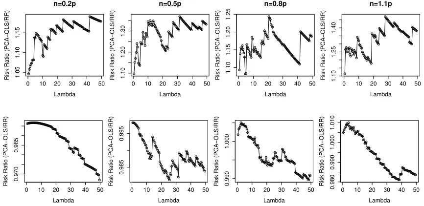
Next , we chose two real world data sets, namely USPS (n=1500, p=241) and BCI (n=400, p=117).2

Since we do not know the true model for these data sets, we used all the n observations to fit an OLS regression and used it as an estimate of the true parameter β. This is a reasonable approximation to the true parameter as we estimate the ridge regression (RR) and PCA-OLS models on a small subset of these observations. Next we choose a random subset of the observations, namely 0.2_×p, 0.5_×pand 0.8_×pto fit the ridge regression (RR) and PCA-OLS models.

The results are shown in Figure 2. As can be seen, the risk ratio of PCA-OLS to ridge regression (RR) is again within a factor of 4 and often PCA-OLS is better, that is, the ratio<1.

4. Conclusion

We showed that the risk inflation of a particular ordinary least squares estimator (on the “top” PCA subspace) is within a factor 4 of the ridge estimator. It turns out the converse is not true — this PCA estimator may be arbitrarily better than the ridge one.

Appendix A.

Proof of Lemma 1.We analyze the bias-variance decomposition in Equation 1. For the variance,

EYkβˆλ−β¯λk2Σ =

∑

j

λjEY([βˆλ]j−[β¯λ]j)2

=

_∑

j

λj

(λj+λ)2 1

n2E

"

n

∑

i=1

(Yi−E[Yi])[Xi]j n

∑

i′₌₁

(Y_i′−E[Y_i′])[X_i′]j

#

=

_∑

j

λj

(λj+λ)2

σ2

n n

∑

i=1

Var(Yi)[Xi]2j

=

_∑

j

λj

(λj+λ)2

σ2

n n

∑

i=1

[Xi]2j

= σ 2

n

∑

_j

λ2

j

(λj+λ)2

.

0 10 20 30 40 50

0.0

0.2

0.4

0.6

0.8

Lambda

Risk Ratio (PCA−OLS/RR)

n=0.2p

0 10 20 30 40 50

0.2

0.6

1.0

Lambda

Risk Ratio (PCA−OLS/RR)

n=0.5p

0 10 20 30 40 50

0.5

0.7

0.9

1.1

Lambda

Risk Ratio (PCA−OLS/RR)

n=0.8p

0 10 20 30 40 50

0.5

0.7

0.9

Lambda

Risk Ratio (PCA−OLS/RR)

n=1.1p

Figure 1: Plots showing the risk ratio as a function of λ, the regularization parameter andn, for the synthetic data set. p=100 in all the cases. The error bars correspond to one standard deviation for 100 such random trials.

0 10 20 30 40 50

1.05

1.10

1.15

Lambda

Risk Ratio (PCA−OLS/RR)

n=0.2p

0 10 20 30 40 50

1.10

1.20

1.30

Lambda

Risk Ratio (PCA−OLS/RR)

n=0.5p

0 10 20 30 40 50

1.10

1.15

1.20

1.25

Lambda

Risk Ratio (PCA−OLS/RR)

n=0.8p

0 10 20 30 40 50

1.10

1.25

1.40

Lambda

Risk Ratio (PCA−OLS/RR)

n=1.1p

0 10 20 30 40 50

0.970

0.985

Lambda

Risk Ratio (PCA−OLS/RR)

0 10 20 30 40 50

0.985

0.995

Lambda

Risk Ratio (PCA−OLS/RR)

0 10 20 30 40 50

0.990

1.000

Lambda

Risk Ratio (PCA−OLS/RR)

0 10 20 30 40 50

0.980

0.990

1.000

1.010

Lambda

Risk Ratio (PCA−OLS/RR)

Similarly, for the bias,

kβ¯λ−βk2Σ =

∑

j

λj([β¯λ]j−[β]j)2

=

_∑

j

β2_jλj

λj

λj+λ− 1

2

=

_∑

j

β2_j λj (1+λj

λ)2

,

which completes the proof.

The risk for RR can be arbitrarily worse than the PCA-OLS estimator.

Consider the standard OLS setting described in Section 1 in whichXisn_×pmatrix andY is a

n_×1 vector.

Let X=diag(√1+α,1, . . . ,1), thenΣ=X⊤X=diag(1+α,1, . . . ,1) for some (α>0) and also chooseβ= [2+α,0, . . . ,0]. For convenience let’s also chooseσ2_=n.

Then, using Lemma 1, we get the risk of RR estimator as

Risk(βˆλ) =



  

1+α

1+α+λ

2

| {z }

I

+ (p−1) (1+λ)2

| {z }

II



 

+ (2+α)

2

× (1+α)

(1+1+α λ )2

| {z }

III

.

Let’s consider two cases

• Case 1:λ<(p₋1)1/3₋1, thenII>(p₋1)1/3.

• Case 2:λ>1, then 1+1+α

λ <2+α, henceIII>(1+α).

Combining these two cases we get _∀λ, Risk(βˆλ)>min((p−1)1/3,(1+α)). If we choose p

such thatp₋1= (1+α)3_{, then Risk(βˆ}

λ)>(1+α).

The PCA-OLS risk (From Theorem 2) is:

Risk(βˆPCA,λ) =

∑

j 1

λj≥λ+

∑

j:λj<λ λjβ2j.

Consideringλ_∈(1,1+α), the first term will contribute 1 to the risk and rest everything will be 0. So the risk of PCA-OLS is 1 and the risk ratio is

Risk(βˆPCA,λ)

Risk(βˆλ)

≤ ₍₁₊1_α).

References

D. P. Foster and E. I. George. The risk inflation criterion for multiple regression. The Annals of Statistics, pages 1947–1975, 1994.