Fault Diagnosis of Discrete-Time Linear Systems Using Continuous Time Delay Petri Nets

Vol. 3, No. 1, pp. 81-90, Jan (2020)

Fault Diagnosis of Discrete-Time Linear

Systems Using Continuous-Time Delay Petri Nets

Sobhi Baniardalani

†

Department of Electrical Engineering, Faculty of Energy, Kermanshah University of Technology, Kermanshah, Iran

This paper deals with the fault diagnosis of a linear continuous variable dynamical system represented by a discrete state-space model. The proposed fault diagnoser was based on a special Petri net (PN) called continuous-time delay Petri net (CTDPN). According to the theorem presented in this paper, an exact correspondence between discrete state-space equations and fundamental equations of the CTDPN was established. Based on this theorem, a systematic method was proposed for the realization of classical parity equations by a CTDPN that played the role of the fault diagnoser. By integrating the concept of state-space models and PNs in this paper, new and effective methods can be proposed for the analysis and fault diagnosis of hybrid systems. Finally, the performance of the proposed method was investigated for the fault diagnosis of a DC motor. The results demonstrated that, with the help of the proposed PN, fault diagnosis can be performed well and the traditional diagnoser can be replaced with this novel network.

Article Info

Keywords:

Continuous-Time Delay Petri Net, Fault Diagnosis, Parity Equations, State-Space Model

Article History: Received 2019-01-11

Accepted 2019-09-29

I.

I

NTRODUCTION

Fault diagnosis and condition monitoring methods in dynamical systems have increasingly been developed in recent years, with numerous methods proposed for a wide range of applications [1, 2]. Some of these methods utilize Petri nets (PNs) [3]. PNs are powerful modeling tools with intuitive graphical representation for the simulation of systems. They also provide a formalism for setting up state equations and algebraic equations governing the behavior of the system [4]. Considering the PN properties, the present paper focused on the fault diagnosis of continuous variable dynamical systems (CVDSs) using a special PN known as the continuous-time delay Petri net (CTDPN). Most studies cited here related to fault diagnosis by PN focused on discrete event systems (DESs) [5-8]. From a formal perspective, a DES can be thought of as a dynamic system whose

state-space is a discrete set and the state transition mechanism is event-driven [9].

However, in the real world, we are faced with CVDSs represented by differential equations or difference equations. These systems cannot be exactly modeled and analyzed by conventional classic PNs. To cope with this limitation, alternative classes of PNs such as continuous, timed continuous, and hybrid PNs have been introduced [4, 10]. In [11, 12] a special type of this class, CTDPN, has been introduced for the modeling and controller design of continuous systems. CTDPN is a continuous PN in which the marking of places can be non-zero real numbers and transitions can be fired if each of their input places has a non-zero marking. In addition, the speed of transitions is infinite. In [12] this PN has been employed to implement the discrete state-space of a dynamic system, and in [11] an approach has been presented to design a state controller based on this PN for a continuous dynamic system.

According to the outstanding features of CTDPN for the simulation of a discrete-time state-space model of a dynamic system, it can be an effective tool for the fault diagnosis of †_{Corresponding Author :[email protected]}

Tel: +98-83-38305000,Fax: +98-83-38305006, Kermanshah University of Technology

A

B

S

T

R

A

discrete-time CVDSs as shown in the present paper. In this paper, a novel approach is presented for the fault diagnosis of a CVDS represented by a discrete-time state-space model. In fact, by the proposed method of this paper, a conventional diagnoser is designed and is then realized by a CTDPN. From this point of view, the proposed method can be regarded as the generalization and development of the algebraic fault diagnosis approach presented for DESs [13-15]. Due to the compatibility of CTDPN with the continuous systems, we can utilize the well-known fault diagnosis methods to design the CTDPN fault diagnoser. In this paper, the discrete-time parity approach has been adopted to generate structured residuals indicating the occurred faults [16]. These residuals are represented by marking of places in the realized CTDPN.

In the past decade, the application of powerful programmable logic controllers (PLCs) has become widespread in various industries [17, 18]. As a result, the idea of implementing an online diagnoser and a feedback controller, both on the same PLC, has received further attention. Some advantages of this implementation scheme are the reduction of hardware needed for diagnosis, no need for the sensor installation to observe command events, no need for communication buses, and a higher fault diagnosis speed [19-21].

A challenging issue in this regard is that the on-line diagnoser system should be easily implemented by a standard PLC programming language. As reported by the few works addressing the problem of implementing online diagnosis on a PLC, PN-based diagnosis has superior compatibility with PLC programming languages such as the ladder diagram (LD) or sequential function chart (SFC) [19-22]. All the studies cited before were on DESs and, to the best of the author’s knowledge, no research has dealt with the problem of implementing online PN-based diagnosers for CVDSs on a PLC. Thus, the main motivations for the present work are as follows:

-The lack of a general framework for implementing the well-known fault diagnosis methods for CVDS on PLCs (This paper proposes an appropriate PN-based diagnosis for these systems as the first and most important step.) -Facilitating access to unified formalism based on PNs for fault diagnosis in hybrid systems exhibiting both continuous and discrete dynamic behaviors.

Related literature

The use of PNs for fault diagnosis systems has been reviewed in a number of papers along with other models such as automata [5-8, 23-26]. In [5], three main methods, including the algebraic method for fault diagnosis, have been investigated. In [13-15], faults in both PN transitions and places have been considered, and a redundant PN has been constructed and attached to the main PN. In the diagnosis scheme in [13], the nonzero marking of redundant places has

been decoded to indicate the occurred faults. Similar to [13], in this paper, we constructed a redundant CTDPN in which the markings of places were equal to residuals indicating the occurred faults. In [27], the faults have been modeled by unobservable transitions and an algorithm has been presented for the separation of the faulty part. In this method, there is no need for a redundant network for fault diagnosis and this is the main advantage of this method over our paper. However, this method is applicable only for pure DESs. In [7, 8] a diagnoser based on the reachability graph has been proposed for bounded PNs (a PN with limited marking value) and analyzed. Since the reachability graph cannot be accessed for continuous PNs, this method is not applicable for CVDSs.

As mentioned before, alternative PNs such as continuous Petri nets (CPNs), timed continuous Petri nets (TCPN), hybrid Petri nets (HPN), and CTDPNs have been introduced to model and analyze continuous dynamic systems [4, 11, 28]. In [28] a survey of using HPNs for logistic purposes has been presented, and in [29] CPNs have been applied for modeling and analyzing biological systems. The major drawback of PNs introduced in [28-30] is that their markings are positive real numbers, and thus these PNs cannot be utilized for modeling CVDSs whose state variables have negative values, while this limitation does not exist in the network employed in the present study.

A few studies have addressed the fault diagnosis in TCPN [31-33]. In [31], a fault modeling framework based on hybrid automata has been presented and an online monitoring approach based on a timed PN model that abstracts away the continuous dynamics has also been described. Contrary to [31], the continuous dynamics was directly simulated by CTDPN in the present paper. Moreover, [32] has implemented an adaptive fault diagnoser for a system modeled by a TCPN under infinite server semantics. This work has proposed a single diagnoser model whose structure was known and some of its parameters were updated depending on the fault occurrence. In this model, identification algorithms, based on heuristic optimization methods, have been used to identify unknown fault parameters.

In comparison with the present study, the method proposed in [32] is more complex and cannot be implemented online by PLCs. In [33], the fault isolation problem has been investigated for the systems modeled by TCPNs under infinite server semantics. In order to isolate faults, a diagnoser based on a set of robust reduced-order finite-time observers has been proposed in this work.

In comparison with the cited works, the main contributions of the present paper are:

-Introducing a novel approach for the fault diagnosis of a CVDS by a CTDPN

-Presenting a direct path to implement conventional quantitative diagnosers by PNs

The remainder of this paper is organized as follows: In Section 2, we present preliminaries and basic definitions. Section 3 illustrates how to convert a discrete state-space model into CTDPN. Section 4 describes the design procedure of diagnosis systems, and Section 5 presents the result of using the proposed diagnoser for a DC motor.

II.

PRELIMINARIES

In this section, some basic definitions required in other sections are reviewed.

A. Discrete PN

Definition 1 [34]:A PN is a structure = ( , , , , ) where = { , , … , } is the set of m places, = { , , … , } is the set of n transitions,

: × → is the pre-incidence function specifying the number of arcs directed from places to transitions (called “pre” arcs) and represented by an m×n matrix, : ×

→ is the post-incidence function specifying the number of arcs directed from transitions to places (called “post” arcs) and represented by an m×n matrix, and is the initial marking. The incidence matrix is equal to = −

. For a transition ∈ , its sets of input and output places are respectively defined as:

• = {p ∈ P | Pre (p, ) > 0}, and •= {p ∈ P | Post (p, ) > 0}, while given a place p ∈ P, its set of input and output transitions are defined as:

•p = { ∈ T | Post (p, ) > 0},p• = { ∈ T | Pre (p, ) > 0}.

Definition 2 [34]:A marking is a function M : P → N that assigns to each place a non-negative integer number of tokens. The marking of a PN defines its state.

Definition 3 [34]:A transition is enabled at a marking M, if M ≥ Pre (·, ), i.e., if each place p ∈ P contains a number of tokens greater than or equal to Pre (p, ).

Definition 4 [34]:A transition enabled at a marking M can fire. The firing of removes Pre (p, ) tokens from each place p ∈ P and adds Post (p, ) tokens in each place p

∈ P, yielding a new marking:

′ = − (. , ) + (. , ) = + (. , ) (1) To denote that the firing of from M leads to ′, we write

[ > ′. Let S be a firing sequence which can be performed from a marking , and suppose that is reachable from by applying S [4, 11]. The characteristic vectorof sequence S, written as s, is the m-component vector whose component number i corresponds to the number of firings of transition in sequence S, i.e.

= + + ⋯ + , (2)

where represents the firing transition of . In this case, is obtained by fundamental equation:

= + . (3)

B. Continuous PN (CPN)

Definition 5 [4]:A marked autonomous continuous PN is a five-tuple = ( , , , , ) such that P and T are the same as Definition 1, : × → and

: × → are the input and output incidence applications, respectively, and : → is the initial marking. , denotes the weight of the arc →

and is a positive real number if the arc exists and 0 otherwise. Similarly, , is the weight of the arc → . In addition, a place marking must be a real number since it may change continuously. In a continuous PN, places and transitions are represented by a double line.

Definition 6 [4]:In a continuous PN, the enabling degree of transition for marking M, denoted by q or q( , M), is the real number q such that

= _{: ∈•} ( )

, . (4) If q > 0, transition is enabled, and it is said to be q-enabled. Definition 6 is applied to a generalized PN. In the particular case of a PN in which the weight is 1 for all input arcs to the transitions, Equ. (5) can be simplified as:

= _{: ∈•} ( ( )) . (5)

Definition 7 [4]: A timed continuous PN (TCPN)is a pair (R, Spe) such that R is a marked autonomous continuous PN (c. f. Definition 5), and Spe indicates a function from the set T of transitions to ∪ {∞}. For each , Spe( )= is the maximal speed associated with transition . The

instantaneous firing speed satisfies the following condition [4]:

≤

For a timed continuous PN, between times and + , the quantity of firing of is ( ). ; then, scorresponds to the vector ( ). . It follows that:

( + ) = ( ) + ∙ ( ), (6) then

( ) = ( ) + ∫ ( ) , (7)

is the fundamental equation for a timed continuous PN. It works for any 0≤ ≤ [4].

C. Continuous-Time Delay Petri Net

Definition 8 [11]: A continuous-time delay Petri net is a timed continuous PN in which each transition firing plays the role of a unit time delay. In fact, in this TCPN, when a transition is enabled, it is fired after a time delay (e.g. ). Moreover, in this PN, the following assumptions are held [11]:

Assumption 1. Place tokens and weights of the arcs in CTDPN can be negative or non-negative real numbers at any time.

Assumption 2. A transition is enabled if ( ) > 0 or

Assumption 3. The speed of the transitions is infinity.

Assumption 4. When transitions are fired, values of tokens of input places become zero.

III.

DYNAMICS

OF

THE

CTDPN

This paper is based on the application of CTDPN for realizing a well-known fault diagnosis system (represented by a set of difference equations). Therefore, in the first step, the CTDPN dynamics should be determined and then the relation between this dynamic and the difference equations must be established. To do this, the following theorem illustrates how the marking vector of a CTDPN changes with time and the enabling degree of the transitions.

Theorem 1: For a given CTDPN, if ( ( ) is the marking vector at time , then (( +1) ) = ( ) +

( ), in which (( +1) ) indicates the marking vector at the time ( + 1) , denotes the incidence matrix, and ( ) = [ ( ) ( ) … ( )]

represents the enabling degree vector of all transitions at time .

Proof: As previously mentioned (c.f. Definition 7), ( )

denotes the mark flow rate of . Therefore, the mark transported by (firing quantity of ), between times and + ∆ , is

∆ = ( ). ∆ . (8)

Since there is no limit to the firing quantity of , ∆ is only limited to the enabling degree of ; it means that

∆ = ( ). Here, ( ) is the enabling degree of and is defined by Equ. (4). As a result, ∆ is finite and, because of the infinity speed of transitions, (c.f. Assumption 3 in section 2.3), it results from Equ. (8) that ∆ → 0. Thus Equ. (8) can be written as:

= ( ). . (9)

It means that when is fired at time instance , the entire marking is transported instantaneously at this time such that:

∆ = ∫ = ( ) = ∫ ( ) . . (10)

Here, = − and = + where → 0.

For a CTDPN with initial enabling degree vector

(0) = [ (0) (0) … (0)] , all transitions can be fired only at instances, where k=1,2,… .Thus Equ. (10) can be rewritten for all transitions as follows:

( ) = ∫ ( ) . , for k=1,2,…. (11)

Here, ( ) denotes the transition speed vector. Now, if Equ. (7) is written for = and = , and also using Equ. (11), then

( ) = ( ) + ∫ ( ) . ,

( ) = ( ) + ( ). (12)

By replacing = and = ( − 1) for k=1,2,…, we have for k=1,2,…

( ) = (( − 1) ) + (( − 1) ), (13) Finally, for k=0,1,…, (13) can be written as

(( +1) ) = ( ) + ( ) (14)

For simplicity, is abbreviated to k henceforth. In addition, to avoid conflict, it is assumed that for each place, its output transitions (e.g. ) have more priority over its input transitions. For further illustration, consider a place that is an input place for and an output place for . At time instance , both transitions are fired simultaneously. According to this assumption, the marking of this place is transported via at first, then it accepts the transported marking from . In the following, a corollary of the presented lemma is given.

Corollary 1: Consider a particular CTDPN in which the weights are 1 for all input arcs to the transitions (e.g.

, = 1 for all and ), and each transition has one and only one input place (e. g • = for all ). From Equ. (5), it is concluded that:

= _{: ∈•} ( ) = ( )). Thus Equ. (14) in the

theorem is simplified as:

( + 1) = ( ) + ( ) . (15)

IV.

FAULT

DIAGNOSER

DESIGN

In the previous sections, CTDPN was introduced and its dynamics were obtained according to Equ.s (14) and (15). In this section, a fault diagnoser is constructed by the particular CTDPN illustrated by Corollary 1 and its dynamic Equ. (15). In the first step, the diagnoser was designed. Here, we used the well-known method of parity equations (briefly reviewed in what follows) to design a fault diagnoser for the continuous system. The results of this stage were the set of parity equations determining residual vector ( ) (c.f. Equ. (19)). In the second step, a CTDPN was constructed to realize the parity equations and obtaining the residual vector. In this step, the state-space equations and parity equations were combined to obtain dynamic equations of the CTDPN (c.f. Equ.s (24) and (25)).

A. Fault diagnoser design with parity equations [35]: A straightforward method for detecting process faults is to compare the process behavior with a process model describing the nominal, i.e. non-faulty behavior. The difference of signals between the process and the model is expressed by residuals. The residuals can be made in state-space formulation and are used to identify the faults occurring in the process. For a given linear system with p inputs, r outputs, and n state variables, the discrete-time state-space model is described by:

( + 1) = ( ) + ( ) + ( ) (16)

in which , , , and denote the state-space matrices,

( ) are additive faults, and and are gain matrices of faults, respectively. ( ) may be compsed of additive faults

( ) on the input, and ( ) are additive faults on the output ( ) = [ ( ) ( )].

For simplicity, it is assumed that = 0 which is true in many real cases and does not basically change the equations. Introducing Equ. (6) to (17) yields

( + 1) = ( ) + ( ) + ( ) + ( ) (18) For the next sampled output, it holds:

( + 2) = ( + 2) + ( + 2)

= ( + 1) + ( + 1) + ( + 1) + ( + 2)

= ( ) + ( ) + ( + 1) + ( ) +

( + 1) + ( + 2)

and for the sample ( ≤ ):

( + ) = ( ) + ( ) + ⋯ + ( + −

1) + ( ) + ( + 1) + ⋯ + ( + −

1) + ( + ). (19)

Equ. (19) gives the redundant equations for different time instants. The equations for a time window of length q+1 ( ≤

) are summarized, leading to:

( + ) = ( ) + ( + ) + ( ), (20) when time is shifted by q backwards

( ) = ( − ) + ( ) + ( − ), (21) with the vectors

( ) = ⎣ ⎢ ⎢ ⎢ ⎢ ⎡ ( − ) ( − + 1)

. . . ( ) ⎦ ⎥ ⎥ ⎥ ⎥ ⎤

, U ( ) =

⎣ ⎢ ⎢ ⎢ ⎢ ⎡ ( − ) ( − + 1)

. . . ( ) ⎦ ⎥ ⎥ ⎥ ⎥ ⎤ ,

F( − ) =

⎣ ⎢ ⎢ ⎢ ⎢ ⎡ ( − ) ( − + 1)

. . . ( ) ⎦ ⎥ ⎥ ⎥ ⎥ ⎤ (22)

and the matrices

= ⎣ ⎢ ⎢ ⎢ ⎢ ⎡ . . . ⎦ ⎥ ⎥ ⎥ ⎥ ⎤ , = ⎣ ⎢ ⎢ ⎢ ⎢ ⎢ ⎡ . . . . . . . . . . . . . . . . … ⎦ ⎥ ⎥ ⎥ ⎥ ⎥ ⎤ and, = ⎣ ⎢ ⎢ ⎢ ⎢ ⎢ ⎡ . . . . . . . . . . . . . . . . … ⎦ ⎥ ⎥ ⎥ ⎥ ⎥ ⎤

. (23)

As the state vector ( − ) is unknown, Equ. (21) is multiplied by a weighting matrix V,

( ) = ( − ) + ( ) + ( − ). (24)

By selecting ×( ) such that VT=0, an input-output relation results. Consequently, residuals are defined as:

( ) = ( ) − ( ) = ( ). (25) In Equ. (25), ( ) includes h residuals. When ( ) = 0, then ( ) becomes zero, meaning that no fault has occurred. If ( ) ≠ 0, then computing ( ) from (25) leads to a nonzero vector. The weighting matrix can be chosen such that the special properties of the residuals, e.g. structured residuals, are obtained. Here, structured residual vectors are generated such that each residual is at least independent from one of the faults. As a result, it is easier to detect the faults by these residuals.

B. Realization parity equations by CTDPN

This subsection describes the procedure of the realization of parity Equ. (25) by a CTDPN that plays the role of the fault diagnoser.

1) For each signal variable in Equ. (25), a place is assigned in the PN. Therefore, the CTDPN marking vector ( )

contains input and output vectors and their q backward is shifted ( . . ( ) and ( ) in Equ. (22)), and also × are the residuals containing h residuals. Thus, the total number of places is = ( + )( + 1) + ℎ.

( ) = [ ( ) ( ) ( )] = [ ( ) ( ) … ( )] .

(26) 2) The relationship between ( ) and ( − 1) is determined using Equ.s (22)-(25). Given the structure of

( ), it can be observed that for input vector ( ), and for

= 0,1, … , , ( ) = ( − + ) (27) where = + = 1, … , . For output vector ( ),

( ) = ( − + ) (28) where = ( + 1) + + and = 1, … , .

For residual vector ( ),

( ) = ( )

= ( + 1) + ( + 1) + , and = 1, … , ℎ. (29)

3) It can be verified that the relationships described by Equ.s (27)-(29) can be written in the form of a matrix equation such that:

( ) = ( − 1), where

= ⎣ ⎢ ⎢ ⎢ ⎢ ⎡ × × × × × × × × × × × × × × × × × × × × − _× ⎦⎥ ⎥ ⎥ ⎥ ⎤

. (30)

Note that ( ) and ( ) are independent of the other signals ( − ) and ( − ). Therefore, Rows 2 and 4 are in matrix H are equal to zero.

4) By using Corollary 1 for this CTDPN,

A

R

Ψ

Ψ

F

M

SJ

1

A

U

L

M



A

I

A

SL

1

Fig. 1. Signal flow graph of the DC motor

For a better explanation of the method presented in this paper, an illustrative example is given in the next section.

V.

AN

ILLUSTRATIVE

EXAMPLE

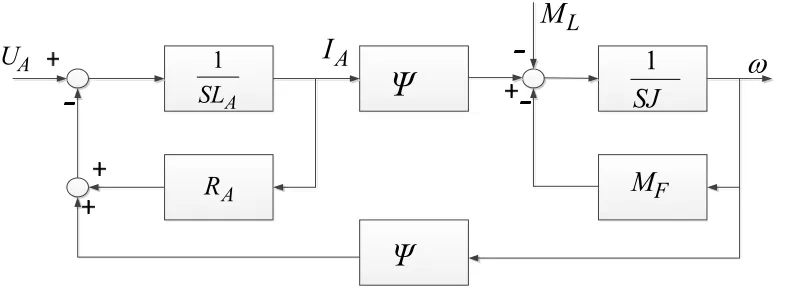
This section presents how to apply the proposed method to implement a fault diagnoser for a DC motor. Here, a permanently excited DC motor with a rated power of P= 550W at rated speed n= 2500 rpm is considered [35]. Fig. 1 depicts the signal flow graph of the motor and its data are given in Table 1.

The linear state-space model of this system becomes

̇ = ̇ ̇ =

− −

− +

0

0 − , (32)

= = 1 0

0 1 .

Thus, the linear discrete-time state-space representation of the DC motor with a sampling time of 0.001 seconds is as follows:

( + 1) = ( + 1) ( + 1) =

0.7966 − 0.0433 0.1538 0.9959

( ) ( ) + 0.1313 0.0117

0.0117 − 0.5201 ( ) ( ).

( ) = = 1 0

0 1 ( ).

(33)

Here, , , and are the measured armature current, armature voltage, and speed of the motor, respectively, and

is the load torque.

From Equ. (27), discrete state-space parameters are obtained as follows:

TABLE I

DATA FOR THE DC MOTOR [35] Armature resistance = 1.52 Ω

Armature inductance = 6.82 ∙ 10

Magnetic flux = 0.33

Voltage drop factor = 2.21 ∙ 10 /

Inertia constant = 1.92 ∙ 10

Viscous friction = 0.36 ∙ 10

= 0.7966 − 0.0433

0.1538 0.9959 , =

0.1313 0.0117 0.0117 − 0.5201 and = 1 0

0 1 .

A. Fault diagnoser design

In this subsection, a fault diagnoser based on Section 4 is designed for the previously mentioned DC motor. The diagnoser is based on parity equations presented in Subsection 4.B. Two faults are considered here, a bias in the armature current sensor (f ) and a bias in the speed sensor (f ). Therefore, two structured residuals (r and r ) should be made such that when a fault occurs, only its corresponding residual remains unchanged and the other residual changes. In [35], a fault diagnoser has been designed for this case, and the results of that work are used here to realize a CTDPN-based fault diagnoser. According to [35], q = 2

and therefore, from Equ. (17), we have:

(k) = [I (k − 2) ω(k − 2) I (k − 1) ω(k − 1) I (k) ω(k)] , (34)

(k) =

[U (k − 2) M (k − 2) U (k − 1) M (k − 1) U (k) M (k)]

(35)

(k) = [r (k) r (k)] . (36) Here, r (k) and r (k) are the residuals corresponding to f

and f , respectively.

M(k) is obtained by substituting Equ.s (34)-(36) in (26) and the matrix Q is computed using Equ. (23) for the matrices A, B, and C of Equ. (32). For generating structured residuals, the weighting matrix V is adapted from [35] as follows:

=

0 0 0

0 0 0

, (37)

where = + and = + . Selecting

this weighting matrix causes the residuals to be independent of one another. Finally, the matrices = and

1

1

1

)

2

(

k



U

_A

1

1

1

1

1

1

1

1

1

1

p

p

2

3

p

p

4

5

p

p

6

8

p

9

p

p

10

12

p

11

p

7

p

1

T

4

T

2

T

5

T

T

₆

3

T

7

T

T

8

9

T

T

10

11

T

T

₁₂

1

1

1

1

1

1

1

1

)

1

(

k



U

_A

)

(

k

M

_L

)

1

(

k



M

_L

)

2

(

k



M

_L

)

1

(

k



I

A

)

2

(

k



I

A

)

(

k

I

A

)

1

(

k





)

2

(

k





)

(

k



1

1

)

(

k

U

_A

13

P

P

14

13

T

T

₁₄

-

J

F

M







A

JL









A

R

A

L





A

JL

)

(

1

k

r

r

₂

(

k

)

Fig. 2. CTDPN fault diagnoser for the DC motor

last two lines of matrix H, which describe the parity equations, are presented.

= [− ] =

− − − 0 0 0 0 0 0 − 0 0 0 0 0 0 .

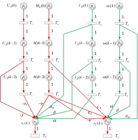
(38) According to Equ. (25), the corresponding CTDPN that plays the role of a fault diagnoser for the main system is obtained and depicted in Fig. 2. In this CTDPN, the places

p and p are redundant places that compute the residuals indicating the faults. The remainder of the network provides the delay timed signals from the inputs and the outputs, required for residual calculations.

The performance of the proposed diagnoser is investigated here in three cases. In all cases, = 24 and = 0.3 are applied to the DC motor.

B. Case 1: Faultless system

No fault occurs in this case. Fig. 3-a shows the residuals generated by the CTDPN fault diagnoser (i.e. ( ) and

( ), the markings of places and in Fig. 2). Evidently, the two residual values converge to zero after a transient time (about 0.2 s), indicating no fault occurrence.

C. Case 2: The armature current sensor fault

current armature due to a fault of the current sensor. It is assumed that the fault affected the sensor at t=0.3 s. Fig. 3-b shows that ( ) remains unchanged, while ( ) is changed abruptly at t=0.3 s, indicating that the fault has occurred at t=0.3 s. For more clarity, the residuals are normalized with respect to their thresholds and depicted for steady-state time ( ≥ 0.2 ).

D. Case 3: The speed sensor fault

This case is similar to Case 2, differing in that only the speed sensor is affected by the same fault of that case. The changes in the residuals are depicted in Fig. 3-c. In this figure,

( ) remains unchanged, whereas ( ) is changed, indicating that occurred at t=0.3s.

VI. COMPARISONWITHSIMILARSTUDIES

A. Classical methods:

The equations used in this paper are the same as the classical equations in fault diagnosis methods such as parity equations [16], but the main feature of this paper is that it provided an intuitive model for implementing classical methods. The use of PNs also provided the capability of developing the proposed method for hybrid systems.

B. Redundant PN diagnoser:

Similar to [13-15], in this paper, we constructed a redundant PN as a diagnoser in which the markings of places were equal to residuals indicating the occurred faults. The main difference between our paper and [13-15] lies in the type of network used and its equations. In this paper, a continuous type of PN was employed with difference equations, while the PNs used in [13-15] were ordinary PNs with algebraic equations for DESs

Differential PNs:

In the literature review, the difference between CTDPN and regular CPNs and HPNs was stated. In [36] a special CPN has been introduced and known as differential Petri nets (DPNs). In a DPN, similar to a CTDPN, markings and arc values can be negative real numbers and are, therefore, suitable for modeling dynamic systems. The main difference between this network and CTDPN is that DPN is applicable for modeling continuous-time dynamical systems and differential equations, whereas CTDPN is suitable for discrete-time systems and difference equations. In [37], DPN is incorporated for modeling a hybrid system, and in [38], it is applied as a state observer for a continuous-time linear switched system.

(a)

(b)

(c )

Fig. 3. Residuals generated by the CTDPN fault diagnoser for a) the faultless system, b) the fault , c) the fault

.

0.2 0.25 0.3 0.35 0.4 0.45 0.5 -0.01

-0.005 0 0.005 0.01

r1,r2

Time (s) r2

r1

0.2 0.25 0.3 0.35 0.4 0.45 0.5 -0.2

0 0.2 0.4 0.6 0.8 1

r1, r2

Time (s) r2

r1

0.2 0.25 0.3 0.35 0.4 0.45 0.5 -0.2

0 0.2 0.4 0.6 0.8 1

r1, r2

Time (s) r2

VII.

C

ONCLUSIONS

In this paper, a new method for detecting the faults of a continuous linear system by a special continuous PN (CTDPN) was presented. Based on this method, one can design a classic fault diagnoser (e. g. parity equation fault diagnoser) and then realize it by a CTDPN. An advantage of this diagnosis system is the ability for implementation on the same PLC that controls the system. The realization of the CTDPN diagnosis system by PLCs, as a relevant future research direction, can lead to a reduction in costs and an increase in the speed of the fault diagnosis of industrial systems.

Another issue related to this paper is the transformation of the difference equations describing the main system to a CTDPN, as will appear in our future studies. From this point of view, the fault diagnoser CTDPN is regarded as a redundant CTDPN, similar to the idea presented in [13] for monitoring faults in DESs. Integrating these two lines of research will result in a unique and general framework for the fault diagnosis of hybrid systems.

A

CKNOWLEDGMENT

Author would like to acknowledge the financial support of Kermanshah University of Technology for this research under grant number S/P/T/1194.

R

EFERENCES

[1] A. Karimabadi, M. E. Hajiabadi, E. Kamyab, A. A. Shojaei,” The effect of condition monitoring of circuit breaker on the reliability and maintenance cost of substation”, IECO, Vol. 2, No. 3, pp. 167-176, July 2019. [2] Z. Gao, C. Cecati, S. X. Ding,” A survey of fault diagnosis

and fault-tolerant techniques—Part I: fault diagnosis with model-based and signal-based approaches”, IEEE Trans. on industrial electronics, Vol. 62, NO. 6, pp. 3757-3767, June 2015.

[3] A. Giua, M. Silva, ”Petri Nets and automatic control: A historical perspective”, Annual Reviews in Control, Vol. 45, pp. 223-239, 2018.

[4] R. David and H. Alla, Discrete, continuous, and hybrid Petri Nets, Springer-Verlag, Berlin Heidelberg, 2010. [5] Dimitri Lefebvre, Diagnosis of discrete event systems with

Petri Nets, chapter 16 of Petri Net, Theory and Applications, Book edited by Vedran Kordic, Vienna, Austria, pp. 534, Feb. 2008.

[6] M. Iordache and P. Antsaklis, “A survey on the supervision of Petri Nets,” DES Workshop PN 2005, Miami, FL, June 21, 2005.

[7] N. Ran, H. Su; A. Giua; and C. Seatzu, ”Codiagnosability analysis of bounded Petri Nets,” IEEE Trans. on Automatic Control, Vol. 63, Issue 4, pp. 1192 – 1199, 2018.

[8] N. Ran, S. Wang, H. Su, and C. Wang,” Fault diagnosis for discrete event systems modeled by bounded Petri Nets,”

Asian Journal of Control, Vol. 19, No. 6, pp. 1–10, Nov. 2017.

[9] C. G. Cassandras and S. Lafortune, Introduction to discrete event systems, Kluwer, 2nd Edition, 2008.

[10] C. Mahulea, C. Seatzu, M. P. Cabasino, and M. Silva, ”Fault diagnosis of discrete event systems using continuous Petri Nets,” IEEE Trans. on Systems, Man, and Cybernetics—PART A: Systems and Humans, Vol. 42, No. 4, pp. 970-984, July 2012.

[11] A. A. Farahani and, A. Dideban, “Continuous-Time Delay-Petri Nets as a new tool to design state-space controller”, Information Technology and control, T. 45, No. 4, pp. 401-411, 2016.

[12] A. Dideban, A. A. Farahani and M. Razavi, “Modeling of continuous systems using modified Petri Net model”, Journal of Modeling and Simulation of Electrical and Electronics Engineering (MSEEE), Vol. 1, No. 2, pp. 19-23, May 2015.

[13] Y. Wu and C. N. Hadjicostis,” Algebraic approaches for fault identification in Discrete-Event Systems,” IEEE Transaction on Automatic Control, Vol. 50, No. 12, pp. 2048-2053, Dec. 2005.

[14] V. Calderaro, C. N. Hadjicostis, A. Piccolo, and P. Siano, “Failure Identification in smart grids based on Petri Net modeling,” IEEE Trans. on Industrial Electronics, Vol. 58, No. 10, pp. 4613-4623, Oct. 2011.

[15] V. Calderaro, V. Gladi, A. Piccolo, and P. Siano,” Protection system monitoring in electric networks with embedded generation using Petri Nets,” International Journal of Emerging Electric Power Systems, Vol. 9, Issue 6, Article 3, 2008.

[16] R. Isermann, Fault-Diagnosis Applications, Springer-Verlag, Berlin Heidelberg 2011.

[17] J. Zaytoon and B.Riera,” Synthesis and implementation of logic controllers–A review,” Annual Reviews in Control, Vol. 43, pp. 152-168, 2017.

[18] W. Bolton, Programmable Logic Controllers, sixth edition, Elsevier, 2015.

[19] F. G. Cabral, M. V. Moreira, O. Diene and J. C. Basilio, “A Petri Net diagnoser for discrete event systems modeled by Finite State Automata,” IEEE Transactions on Automatic Control Vol. 60, Issue: 1,pp. 59 - 71, Jan. 2015. [20] A. D. Vieira, E. A. P. Santos, M. H. de Queiroz, A. B. Leal, A. D. de Paula Neto; J. E. R. Cury,” A Method for PLC implementation of supervisory control of discrete event systems”, IEEE Trans. on Control Systems Technology, Vol. 25, No. 1, pp. 175-191, JAN, 2017.

[21] J. C. Quezada, J. Medina, E. Flores, J. C. Seck Tuoh, A. E. Solís, V. Quezada,” Simulation and validation of diagram ladder—Petri Nets”, The International Journal of Advanced Manufacturing Technology, Vol. 88, Issue 5–8, pp. 1393–1405, February 2017.

[22] P. Nazemzadeh, A. Dideban and, M. ZareieeA., “Fault modeling in discrete event systems using Petri Nets”, ACM Transactions on Embedded Computing Systems (TECS) - Special Issue on Modeling and Verification of Discrete Event, Vol. 12, Issue 1, Article No. 12, Jan. 2013. [23] X. Wang, C. Mahulea and M. Silva,” Diagnosis of Time Petri Nets using fault diagnosis graph”, IEEE Transaction on Automatic Control, Vol. 60, No., pp. 92321- 2335, September 2015.

Generation, Transmission & Distribution, Vol: 12, Issue: 2, pp. 295–302, 2018

[25] J. Zaytoon, S. Lafortune, “Overview of fault diagnosis methods for Discrete Event Systems, Annual Reviews in Control Vol. 37, pp. 308–320, 2013.

[26] Baniardalani S. and Askari, J.," Fault diagnosis of timed discrete event systems using Dioid Algebra", IJCAS, Vol. 11, No. 6, pp. 1095-1105, Dec. 2013.

[27] G. Zhu, Z. Li, N. Wu, and A. Al-Ahmari,” Fault identification of discrete event systems modeled by Petri Nets with unobservable transitions,” IEEE Tans on systems, man, and cybernetics: Systems 2, pp., 333-345, Feb 2019.

[28] G. Cavone, M. Dotoli, and C. Seatzu, “A survey on Petri Net models for freight logistics and transportation systems,” IEEE Trans on intelligent transportation systems, Vol. 19, Issue: 6, pp. 1795-1813, June 2018.

[29] M. A. Drighiciu,” Hybrid Petri Nets a framework for hybrid systems modeling,” 2017 International Conference on Electromechanical and Power Systems, 11-13 Oct. 2017, Lasi, Romania.

[30] G. Russo, M. Pennisi, R. Boscarino and F. Pappalardo,” Continuous Petri Nets and microRNA analysis in melanoma,” IEEE/ACM Transactions on Computational Biology and Bioinformatics, Vol. 15, Issue 5, pp. 1492-1499, 2018.

[31] F. Zhao, X. Koutsoukos, H. Haussecker, J. Reich and P. Cheung,” Monitoring and fault diagnosis of hybrid systems,” IEEE Trans. on Systems, Man, and Cybernetics—PART A: Systems and Humans, Vol. 35, NO. 6, pp. 1225-1239, Dec. 2005.

[32] R. Casas-Carrillo, O. Begovich, J. Ruiz-Le´on, and S. Cˇ elikovsky,” Adaptive fault diagnoser based on PSO algorithm for a class of Timed Continuous Petri Nets,” IEEE 21st International Conference on Emerging Technologies and Factory Automation, Germany, 6-9 Sept., 2016.

[33] J. A. Fraustro, J. Ruiz-Le´on, C.R. V´azquez, A. R. Trevino, ”Structural fault diagnosis in timed continuous Petri Nets” Proceedings of the 13th International Workshop on Discrete Event Systems, Xi'an, China, May 30 - June 1, 2016.

[34] C. Seatzu, M. Silva, and J. H. van Schuppen, Control of Discrete-Event Systems, Springer-Verlag London 2013. [35] R. Isermann, Fault-Diagnosis Systems, Springer-Verlag

Berlin Heidelberg 2006.

[36] I. Demongodin and N. T. Koussoulas,” Differential Petri Nets: Representing Continuous Systems in a Discrete-Event World,” IEEE Trans on automatic control, Vol. 43, No. 4, pp. 573-579, April 1998.

[37] G. Davrazos, and N. T. Koussoulas,” Modeling and stability analysis of state-switched hybrid systems via Differential Petri Nets,” Simulation Modeling Practice and Theory 15 pp. 879–893. (2007)

[38] F. Hamdi, N. Messai, and N. Manamanni, “State Estimation for switched systems described by differential Petri Nets Models,” Proceedings of the 3rd International Conference on Systems and Control, Algiers, Algeria, October 29-31, 2013.

Sobhi Baniardalani was born in Kermanshah, Iran. He received his B.Sc.

degree in Electronics Engineering from Isfahan University of Technology, Isfahan, Iran, in 1989, and his M.S. degrees in Electronics Engineering from Amirkabir University of Technology, in 1994, and, the Ph.D. degree from Isfahan