Available online at http://scik.org
J. Math. Comput. Sci. 7 (2017), No. 2, 292-306 ISSN: 1927-5307
BAYESIAN ESTIMATION FOR A MULTI STEP-STRESS ACCELERATED GENERALIZED EXPONENTIAL MODEL WITH TYPE-II CENSORED DATA
G. H. ABD EL-MONEM∗, Z. F. JAHEEN
Department of Mathematics, Faculty of Science, Assiut University, Assiut, Egypt
Copyright c2017 G. H. Abd El-Monem and Z. F. Jaheen. This is an open access article distributed under the Creative Commons Attribution
License, which permits unrestricted use, distribution, and reproduction in any medium, provided the original work is properly cited.
Abstract. We consider multiple step-stress accelerated life tests (SS-ALTs) assuming that the lifetime follows a
generalized exponential distribution. Based on Type-II censored data, we calculate the maximum likelihood and
Baysian estimates using MCMC. A Monte Carlo simulation study is carried out to examine the performance of the
maximum likelihood and Baysin estimators through their mean squared error.
Keywords: multi-stress accelerated life tests; generalized exponential distribution; type-II censoring; maximum
likelihood estimation; MCMC estimation; Monte Carlo simulation.
2010 AMS Subject Classification:62N05.
1. Introduction
Many modern electro-mechanical materials and items tend to have a long life under normal-use operating conditions. Hence it is difficult to test their failure times since standard testing procedures are far too lengthy and expensive to be useful. However, accelerated life tests (ALTs)
∗Corresponding author
E-mail address: [email protected]
Received December 6, 2016; Published March 1, 2017
offer an alternative that manufacturing industries prefer due to the ability to obtain enough failure data in a short period of time.
In an ALT the test items are subjected to higher than usual levels of stress to induce early failures. The stress can be applied in different ways including the constant stress and step stress techniques. A step stress ALT is often preferred to a constant stress ALT because it reduces overall test time and enables quicker failures see [5-8]. We consider here m-step stress ALTs wherenidentical units are placed on a life-test with an initial stress levelx1 which is changed
tox2at a fixed timeτ1and the successive failure times are recorded. Then, at the fixed timeτ2,
the stress is increased tox3. Thus the resulting failure times are observed in a naturally ordered
manner.
Cumulative exposure models are often useful in the analysis of step-stress experiments. These models relate the life distribution of the test units at one stress level to the distributions at preceding stress levels by assuming that the residual lives of the experimental units depend only on the cumulative exposure that the units have experienced, with no memory of how the stress was accumulated. Moreover, the surviving units will fail according to the cumulative distribution at the same stress level that is currently being tested at, but starting at the previous accumulated stress level. For more discussion see [1].
We develop a model for 3-step stress ALTs based on the lifetime distribution following a gen-eralized exponential distribution see [2]. We then show how the observed ordered failure times can be used to do maximum likelihood estimation and Baysian estimation of the parameters of the distribution of failure times under normal operating conditions see [9,10]. Finally, we study the performance of these methods in a simulation study under Type-II censoring.
2. Model description
We assume that the lifetimeT follows a two-parameter generalized exponential distribution, denoted GE(α,λ)whereλ is a scale parameter andα is a shape parameter. The two-parameter
The GE(α,λ) probability density function (pdf) and cumulative distribution function (cdf) are given, respectively, by
f(t;α,λ) =α λ(1−e−λt)α−1e−λt, α,λ >0. (2.1) and
F(t;α,λ) = (1−e−λt)α. (2.2) The survival (sf) and hazard rate functions (hrf) are
¯
F(t;α,λ) =1−(1−e−λt)α, (2.3)
and
h(t;α,λ) =α λ(1−e
−λt)α−1e−λt
1−(1−e−λt)α . (2.4)
respectively. For any λ the GE distribution has an increasing hrf if α >1, while the hrf is decreasing ifα<1. Of course, ifα =1, then the hrf is constant.
2.1. Basic assumptions
We assume that the lifetime distribution functions at stress levelsx1,x2andx3areF1,F2and
F3, respectively, and that they belong to the same family of distributions. The experiment starts
withnidentical units, and each unit is subjected to an initial stressx1with lifetimes following the CDFF1(t). The time at which a unit failed will be collected and the surviving units will continue until time τ1at which the stress is increased tox2 and the units will follow the CDF F2(t), once again the time at which a unit failed will be collected and the surviving units will
continue until time τ2at which the stress is increased tox3 and the units will follow the CDF F3(t), but it will start at the previously accumulated fraction failed.
Thus the change in stress level fromx1to x2 changes the lifetime distribution at stress level
x2fromF2(t)toF2(t−τ1+τˆ1), also the change in stress level fromx2tox3changes the lifetime
distribution at stress levelx3fromF3(t)toF3(t−τ2+τˆ2)where F1(τ1) =F2(τˆ1).
F2(τ2) =F3(τˆ2).
Assuming thatλ1,λ2andλ3are the scale parameters associated withF1,F2andF3, respectively,
and assuming absolute continuity of the cumulative distribution function of the lifetime, we find ˆ
τ1=
λ1
λ2
τ1.
ˆ τ2=
λ2
λ3
[τ2−τ1+
λ1
λ2
τ1].
(2.6)
Then, the cumulative distribution function of the model, in which there are three stress levels
x1,x2andx3, will become
G(t) =
G1(t) =F1(t), for 0<t<τ1 G2(t) =F2(t−τ1+τˆ1) for τ1≤t <τ2 G3(t) =F3(t−τ2+τˆ2) for τ2≤t <∞
(2.7)
where
Fi(t) = (1−e−λit)α,i=1,2,3.
The corresponding probability density function (PDF) in this case will be in the flowing form:
g(t) =
g1(t) =α λ1(1−e−λ1t)α−1e−λ1t, 0<t<τ1 g2(t) =α λ2(1−e−λ2(t−τ1+τˆ1))α−1e−λ2(t−τ1+τˆ1) τ1≤t <τ2,
g3(t) =α λ3(1−e−λ3(t−τ2+τˆ2))α−1e−λ3(t−τ2+τˆ2) τ2≤t <∞.
(2.8)
3. Maximum likelihood estimation
In a 3-step-stress model with Type-II censoring, we start with n independent and identical units placed simultaneously on a life-test. Each unit will be subjected to an initial stress level
x1, then the experiment will run until a fixed timeτ1when the stress level is changed tox2, after
that the experiment will run until a fixed time τ2 when the stress level is changed to x3. The
experiment is continued until a specified number of failuresris observed.
Letn1be the number of units that fail beforeτ1,n2 be the number of units that fail between
τ1 andτ2andn3 is the number of units that fail afterτ2, and sor=n1+n2+n3. Ifr failures
occur beforeτ1orτ2, then the test is terminated, otherwise the experiment continues after time
τ2until the requiredrfailures are observed. The ordered failure times that are observed will be
The likelihood function based on the censored data above is given by
L(α,λ1,λ2,λ3;t) = n!
r!{
r
∏
i=1
g(ti)(1−G(tr))n−r}, (3.1)
wherer=n1+n2+n3 and tis the vector of observed Type-II censored data. The likelihood function ofα ,λ1,λ2andλ3is as follows:
(1) Ifn1=0:
L(α,λ2,λ3;t) = n!
r!{
n2
∏
i=1
g2(yi)}{
r
∏
i=n2+1
g3(zi)}(1−G3(zr))n−r
= n!
r!α
r
λ2n2λ3n3e−λ2∑
n2
i=1yi−λ3∑
r i=n2+1zi
× {
n2
∏
i=1
(1−e−λ2yi)α−1}{ r
∏
i=n2+1
(1−e−λ3zi)α−1}
×(1−(1−e−λ3zr)α)n−r
(3.2)
(2) Ifn2=0:
L(α,λ1,λ3;t) = n!
r!{
n1
∏
i=1
g1(ti)}{
r
∏
i=n1+1
g3(zi)}(1−G3(zr))n−r
= n!
r!α
r
λ1n1λ3n3e−λ1∑
n1
i=1ti−λ3∑ri=n1+1zi
× {
n1
∏
i=1
(1−e−λ1ti)α−1}{ r
∏
i=n1+1
(1−e−λ3zi)α−1}
×(1−(1−e−λ3zr)α)n−r
(3.3)
(3) Ifn3=0:
L(α,λ1,λ2;t) = n!
r!{
n1
∏
i=1
g1(ti)}{ n1+n2
∏
i=n1+1
g2(yi)}
= n!
r!α
r
λ1n1λ2n2e−λ1∑
n1
i=1ti−λ2∑n1 +n2 i=n1+1yi
× {
n1
∏
i=1
(1−e−λ1ti)α−1}{
n1+n2
∏
i=n1+1
(1−e−λ2yi)α−1}
(4) Ifni>0 ,i=1,2,3:
L(α,λ1,λ2,λ3;t) = n!
r!{
n1
∏
i=1
g1(ti)}{
n1+n2
∏
i=n1+1
g2(yi)}{
r
∏
i=n1+n2+1
g3(zi)}(1−G3(zr))n−r
= n!
r!α
r
λ1n1λ2n2λ3n3e−λ1∑
n1
i=1ti−λ2∑ni=1+n1n+21yi−λ3∑ri=n1+n2+1zi
× {
n1
∏
i=1
(1−e−λ1ti)α−1}{
n1+n2
∏
i=n1+1
(1−e−λ2yi)α−1}
× {
r
∏
i=n1+n2+1
(1−e−λ3zi)α−1}(1−(1−e−λ3zr)α)n−r
(3.5)
whereyi=ti−τ1+τˆ1 , zi=ti−τ2+τˆ2.
As we can see from (3.2)-(3.5) the three MLEs does not exist unless whenn1,n2,n3>0 and may be obtained by maximizing the corresponding likelihood function (3.5).
Maximizing the likelihood function for the parameters cannot be achieved analytically. The only option we have is to numerically maximize the likelihood function for the vector of param-eters(α,λ1,λ2,λ3). For this purpose, it is convenient to work with the log-likelihood function
rather than the likelihood function in (3.5), which is given by
`(α,λ1,λ2;t) =logc+rlogα+n1logλ1+n2logλ2+n3logλ3−λ1 n1
∑
i=1 ti
−λ2 n1+n2
∑
i=n1+1
yi−λ3 r
∑
i=n1+n2+1
zi+ (α−1)
n1
∑
i=1
(1−e−λ1ti)
+ (α−1)
n1+n2
∑
i=n1+1
(1−e−λ2yi) + (α−1)
r
∑
i=n1+n2+1
(1−e−λ3zi)
+ (n−r)log(1−(1−e−λ3zr)α).
(3.6)
The likelihood equations for the parametersα,λ1,λ2andλ3are given, respectively, by
∂` ∂ α = r α + n1
∑
i=1
(1−e−λ1ti) +
n1+n2
∑
i=n1+1
(1−e−λ2yi) +
r
∑
i=n1+n2+1
(1−e−λ3zi)
−(n−r)(1−e
−λ3zr)αlog(1−e−λ3zr) 1−(1−e−λ3zr)α ,
(3.7)
∂`
∂ λ1
= n1 λ1
+
n1
∑
i=1
{−ti+(α−1)tie
−λ1ti
∂`
∂ λ2
= n2 λ2
+
n1+n2
∑
i=n1+1
{−yi+(α−1)yie
−λ2yi
1−e−λ2yi }, (3.9)
∂`
∂ λ3
=n3 λ3
+
r
∑
i=n1+n2+1
{−zi+(α−1)zie
−λ3zi
1−e−λ3zi } −(
n−r)αzre
−λ3zr(1−e−λ3zr)α−1
1−(1−e−λ3zr)α . (3.10)
The maximum likelihood estimates must be derived numerically because there is no obvious solution of these four non-linear likelihood equations. We used the R software to carry out a numerical maximization on the log likelihood function and obtain the MLEs using the following algorithm:
(1) Simulatenorder statistics from the uniform (0,1) distribution, (U1,U2, ...,Un).
(2) Findn1such thatUn1≤G1(τ1)≤Un1+1. (3) Fori≤n1Ti=−1
λ1ln(1−U 1 α
i ).
(4) Findn2such thatUn1+n2≤G2(τ2)≤Un1+n2+1. (5) Fori≤n1+n2Ti=−1
λ2ln(1−U 1 α
i ) +τ1−τˆ1.
(6) Forn1+n2+1≤i≤rsetTi=−λ1
3ln(1−U 1 α
i ) +τ2−τˆ2.
(7) Obtain the MLEs of(α,λ1,λ2,λ3)based on(T1,T2, ...,Tn1,Tn1+1, ...,Tn1+n2,Tn1+n2+1, ...,Tr) say ˆα,λˆ1,λˆ2and ˆλ3.
(8) Repeat steps 2-7 1000 times.
(9) Compute the MSE of the obtained estimates.
4. Baysian Estimation
There is a fundamental difference between classical and Bayesian estimation. In classical estimation we consider the unknown parameter as a fixed value. But in Bayesian estimation we treat the parameter as a random variable. It is assumed that the parametersα,λ1,λ2andλ3are
π1(α) =
µ1ν1
Γ(ν1)
αν1−1e−µ1α,
µ1,ν1>0,
π2(λ1) =
µ2ν2
Γ(ν2)
λ1ν2−1e−µ2λ1, µ2,ν2>0,
π3(λ2) =
µ3ν3
Γ(ν3)
λ2ν3−1e−µ3λ2, µ3,ν3>0,
π4(λ3) =
µ4ν4
Γ(ν4)
λ3ν4−1e−µ4λ3, µ4,ν4>0.
(4.1)
Then the joint prior density function is
Π(α,λ1,λ2,λ3) =
µ1ν1µ2ν2µ3ν3µ4ν4
Γ(ν1)Γ(ν2)Γ(ν3)Γ(ν4)
αν1−1λ1ν2−1λ2ν3−1λ3ν4−1e−µ1α−µ2λ1−µ3λ2−µ4λ3
(4.2) And hence the posterior function will be as the following
z(α,λ1,λ2,λ3;t)∝ Π(α,λ1,λ2,λ3)L(α,λ1,λ2,λ3;t)
∝ µ ν1 1 µ ν2 2 µ ν3 3 µ ν4 4
Γ(ν1)Γ(ν2)Γ(ν3)Γ(ν4)
αν1−1λ1ν2−1λ2ν3−1λ3ν4−1e−µ1α−µ2λ1−µ3λ2−µ4λ3
×n!
r!α
r
λ1n1λ2n2λ3n3e−λ1∑
n1 i=1ti−λ2∑
n1+n2
i=n1+1yi−λ3∑
r
i=n1+n2+1zi
× {
n1
∏
i=1
(1−e−λ1ti)α−1}{
n1+n2
∏
i=n1+1
(1−e−λ2yi)α−1}
× {
r
∏
i=n1+n2+1
(1−e−λ3zi)α−1}(1−(1−e−λ3zr)α)n−r
(4.3) It is obvious from the posterior function that we are not going to be able to estimate the pa-rameters by the traditional Bayesian methods with integration, so we are going to use one of the MCMC methods which attempt to simulate direct draws from some complex distribution of interest. MCMC approaches are so-named because one uses the previous sample values to randomly generate the next sample value. Here we are going to use the Metropolis algorithm.
Suppose you want to obtain M samples from a univariate distribution with probability density function f(θ,t). Supposeθiis thei−thsample from f. To use the Metropolis algorithm, you
makes a decision to either accept or reject the new sample. If the new sample is accepted, the algorithm repeats itself by starting at the new sample. If the new sample is rejected, the algorithm starts at the current point and repeats. The algorithm is self-repeating, so it can be carried out as long as required.The most common choice of the proposal distribution is the normal distribution N(θi,σ) with a fixedσ. The Metropolis algorithm can be summarized as follows:
(1) Seti=0. Choose a starting pointθo. This can be an arbitrary point as long as f(θo,t)> 0.
(2) Generate a new sample,θnew, by using the proposal distributionq(.|θi).
(3) Calculate the following quantityw=min[f(θnew|t) f(θi|t) ,1]. (4) Sampleufrom the uniform distributionU(0,1). (5) Setθi+1=θnew ifu<w; otherwise setθi+1=θi.
(6) Seti=i+1. Ifi<M, the number of desired samples, return to step 2. Otherwise, stop. The number of iterations used to calculate the MCMC estimates is 50000.
The performance of the MLEs and the Bayes estimates are evaluated using a simulation study in the next section.
5. Simulation study
A simulation study was carried out for different values ofτ1andτ2in order to examine MSE
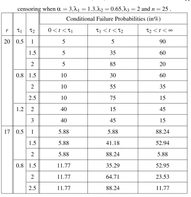
Table 1: Conditional Failure Probabilities (in %) for a multi-stress model under Type-II censoring whenα=3,λ1=1.3,λ2=0.65,λ3=2 andn=25 .
Conditional Failure Probabilities (in%)
r τ1 τ2 0<t<τ1 τ1<t<τ2 τ2<t<∞
20 0.5 1 5 5 90
1.5 5 35 60
2 5 85 20
0.8 1.5 10 30 60
2 10 55 35
2.5 10 75 15
1.2 2 40 15 45
3 40 45 15
17 0.5 1 5.88 5.88 88.24
1.5 5.88 41.18 52.94
2 5.88 88.24 5.88
0.8 1.5 11.77 35.29 52.95
2 11.77 64.71 23.53
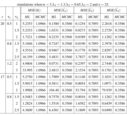
Table 2: The MSE of the MCMC and ML estimates ˆα,λˆ1,λˆ2and ˆλ3based on 1000
simulations whenα =3,λ1=1.3,λ2=0.65,λ3=2 andn=25.
MSE(αˆ) MSE(λˆ1) MSE(λˆ2) MSE(λˆ3)
r τ1 τ2 ML MCMC ML MCMC ML MCMC ML MCMC
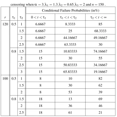
Table 3: Conditional Failure Probabilities (in %) for a multi-stress model under Type-II censoring whenα =3,λ1=1.3,λ2=0.65,λ3=2 andn=150 .
Conditional Failure Probabilities (in%)
r τ1 τ2 0<t<τ1 τ1<t<τ2 τ2<t<∞
120 0.5 1 6.6667 8.3333 85
1.5 6.6667 25 68.3333
2 6.6667 44.16667 49.16667
2.5 6.6667 63.3333 30
0.8 1.5 15 10.83333 74.16667
2 15 30 55
2.5 15 50.83333 34.16667
3 15 65.83333 19.16667
100 0.5 1 8 10 82
1.5 8 30 62
2 8 53 39
0.8 1.5 18 13 69
2 18 36 46
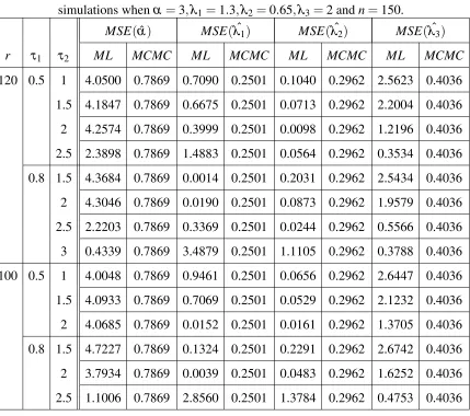
Table 4: The MSE of the MCMC and ML estimates ˆα,λˆ1,λˆ2and ˆλ3based on 1000
simulations whenα =3,λ1=1.3,λ2=0.65,λ3=2 andn=150.
MSE(αˆ) MSE(λˆ1) MSE(λˆ2) MSE(λˆ3)
r τ1 τ2 ML MCMC ML MCMC ML MCMC ML MCMC
6. Concluding Remarks
We have considered multiple step-stress accelerated model when the observed failure times come from aGE(α,λ)distribution under type-II censoring. A simulation study, based on two different examples, was performed to examine the performance of the mean square error of the maximum likelihood and Bayesian estimates.
In Tables 1 and 3, we can see that for a fixed τ1 and increasing τ2 the conditional failure
probabilities occurring on the first level of stress in the interval 0<t <τ1is the same. on the
meanwhile those occurring on the second and third levels of stress change. Asτ2increases the
conditional failure probabilities in the intervalτ1<t<τ2increase ,but decrease inτ2<t<∞.
This means that asτ2increases, there will be more failures occurring beforeτ2and less failures
occurring after it, which means more information aboutλ2and less information aboutλ3. We
also can see that asτ1increases the conditional failure probabilities occurring on the first level
of stress in the interval 0<t<τ1also increase.
In Tables 2 and 4, we can see that the MSEs of the Bayesian estimates of the parameters α,λ1,λ2 andλ3 doesn’t change for different values ofr,τ1orτ2, they only change for different
sample sizesn. On the other hand any change in those values affects the MSEs of the maximum likelihood estimates. In general we can say that MCMC is abetter method to estimate our model parameters in either small and larg sample sizes.
Conflict of Interests
The authors declare that there is no conflict of interests.
Acknowledgements
The first author wishes to thank the Egyptian Ministry of Higher Education and Scientific Re-search for supporting her visiting scholar to the University of Minnesota and Galin Jones for helpful conversations about this paper.
REFERENCES
[1] Wayne Nelson, Accelerated Testing: Statistical Models, Test Plans and Data Analyses, John Wiley & Sons,
[2] Gupta, R. D. and Kundu, D., Generalized exponential distribution, Australian and New Zealand Journal of
Statistics. 41 (1999), 173-188.
[3] Gupta, R. D. and Kundu, D., Generalized exponential distributions: Different methods of estimation, Journal
of Statistical Computation and Simulation. 69 (2001), 315-338.
[4] Gupta, R.D., Exponentiated Exponential Family: An Alternative to Gamma and Weibull Distributions,
Bio-metrical Journal. 43 (2001), 117-130.
[5] Balakrishnan, N. and Kundu, D. and Ng, H. K. T. and Kannan, N., Point and interval estimation for a simple
step-stress model with type II censoring, Journal of Quality Technology. 39 (2007), 35-47.
[6] Nelson, W., Residuals and their analysis for accelerated life tests with step and varying stress, IEEE
Transac-tions on Reliability. 57 (2008), 360-368.
[7] Wu, S. J. and Lin, Y. P. and Chen, S. T., Optimal step-stress test under type I progressive group-censoring
with random removals, Journal of Staistical Planning and Inference. 138 (2008), 817-826.
[8] Abdel-Hamid, A. H. and Al-Hussaini, E. K., Estimation in step stress accelerated life tests for the
exponenti-ated exponential distribution with type-II+ censoring, Computational Statistics and Data Analysis. 53 (2009),
1328-1338.
[9] Jaheen, Z. F. and Moustafa, H. M. and AbdEl-monem, G. H., Bayes Inference in Constant Partially
Accel-erated Life Tests for the Generalized Exponential Distribution with Progressive Censoring, Communications
in Statistics - Theory and Methods. 43 (2014), 2973-2988.
[10] AbdEl-monem, G. H. and Jaheen, Z. F., Maximum likelihood estimation and bootstrap confiedence intervals
for a simple step-stress accelerated generalized exponential model with type II censored data, Far East Journal