Adaptive Region Embedding for Text Classification

(1)

The Thirty-Third AAAI Conference on Artificial Intelligence (AAAI-19)

Adaptive Region Embedding for Text Classification

Liuyu Xiang,

1

_{Xiaoming Jin,}

1

_{Lan Yi,}

2

_{Guiguang Ding}

1 1_{School of Software, Tsinghua University, Beijing, China}

2_{Department of DevNet, Cisco Systems}

[email protected], [email protected], [email protected], [email protected]

Abstract

Deep learning models such as convolutional neural networks and recurrent networks are widely applied in text classifica-tion. In spite of their great success, most deep learning mod-els neglect the importance of modeling context information, which is crucial to understanding texts. In this work, we

pro-pose theAdaptive Region Embeddingto learn context

repre-sentation to improve text classification. Specifically, a meta-networkis learned to generate a context matrix for each re-gion, and each word interacts with its corresponding context matrix to produce the regional representation for further clas-sification. Compared to previous models that are designed to capture context information, our model contains less parame-ters and is more flexible. We extensively evaluate our method on 8 benchmark datasets for text classification. The experi-mental results prove that our method achieves state-of-the-art performances and effectively avoids word ambiguity.

Introduction

Text classification is a fundamental task in many NLP applications such as web searching, information retrieval and sentiment analysis. One key challenge in text classi-fication is to understand the compositionality in text se-quences for which the modeling of regional relationships between words and their neighbours is crucial. Traditional methods usually exploit n-grams as composition function, which proves to be effective by directly gathering adja-cent words. With the emerging development of deep learn-ing, a variety of deep models are recently used for text classification. The most commonly used models are Recur-rent Neural Networks (RNNs) (Tang, Qin, and Liu 2015; Yang et al. 2016; Zhou et al. 2016) and Convolutional Neu-ral Networks (CNNs) (Kim 2014; Zhang, Zhao, and LeCun 2015). RNN and its variants LSTM/GRU model the regional relationships by encoding the previous words into its hidden unit while CNN captures the compositional structure by lay-ers of convolution and pooling. In spite of their success on various NLP tasks, RNNs and CNNs are only generic mod-els for sequences or images. They may neglect the intrinsic semantic relations in text sequences and often require large computational cost and memory space.

Subsequently, several simple and effective models have been proposed to improve the text classification by learn-ing a specially designed high-level representation that con-tains the necessary regional context information. Here we loosely refer to these learned compositional representations as ‘Region Embedding’. Among these methods, (Johnson and Zhang 2015b) learn three types of region embeddings and feed them to a CNN as extra inputs. The region embed-dings help to improve the error rates by a significant margin compared to vanilla CNN. Qiao et al. (2018) propose a two-layer architecture, and introduce a matrix called ‘Local Con-text Unit’ to produce region embeddings. They achieve com-parable or even superior performances to a 29-layer CNN (Conneau et al. 2017), which is the current state-of-the-art method.

Although Qiao et al. (2018)’s region embedding method is able to effectively capture rich context information, it still has the following limitations. First, the region embedding is generated by word embedding and Local Context Unit, where both of them are only and uniquely determined by word indices in the vocabulary. Such embedding method lacks the capability to capture the semantic ambiguity since each word has the same unique region embedding even un-der different contexts.

Second, its representation capability is limited by the fact that the Local Context Unit is generated within just a fixed-length region. This leads to the negligence of richer depen-dencies outside the region. Third, the embedding look-up tensor that generates Local Context Unit is of size E ∈ Rv×h_{, where} _{v, h} _{are sizes of vocabulary and embedding} dimension, respectively. For dataset such as Yahoo Answer with ˜300k words in the vocabulary, i.e. v ≈ 300k, the storage of embedding matrix E requires large memory re-sources.

To address the limitations of Qiao et al. (2018)’s method, we need to design a light-weighted and flexible network component which is able to take the whole sequence into account, and produce effective region embedding adaptive to different contexts.

(2)

gener-ate the context matrix (or context unit) for each small region of texts. Then the region embedding is produced by both the context unit and the word embeddings in the correspond-ing region. The meta-network we use here can be ofany form of fully differentiable neural network that can be jointly trained end-to-end. Our meta-network only requires a tiny amount of parameters, leading to much smaller mem-ory cost. We call our context unit generated by the meta-network Adaptive Context Unit to distinguish from Local Context Unit(Qiao et al. 2018). For simplicity, we refer to Local Context Unit and Adaptive Context Unit asLCUand ACU, and Local Region Embedding and Adaptive Region Embedding asLREandARErespectively in the following discussion.

We compare our method with Qiao et al. (2018)’s and previous state-of-the-art methods on eight benchmark text classification datasets. The experimental results demonstrate that our method is able to achieve state-of-the-art results with much less parameters than Qiao et al. (2018)’s method. Apart from the experimental superiority, we also try to explore the mechanisms behind. We study the differences and relationships between our method, Qiao et al. (2018)’s method and the normal convolution, and generalize them to instance-level, word-level, dataset-level respectively from the perspective ofGeneralized Text Filtering. This general-ization partly explains why our proposed method is more flexible and performs better.

To sum up, the main purpose of this work is to learn a more flexible and compact region embedding. Our main contributions are threefold:

• We propose a new region embedding method where richer context information is acquired through a meta-network.

• Our method achieves state-of-the-art performances on several benchmark datasets with a small parameter space. We also demonstrate that our model is able to avoid word ambiguity.

• We generalize convolution, Qiao et al. (2018) and our method under the same framework, which reveals the mechanisms accounting for our method’s superiority.

Related Work

Text Classification

Text classification has long been studied in Natural Lan-guage Processing. Before the deep learning era, traditional methods usually consist of high-dimensional features fol-lowed by classifiers such as SVM and logistic regression (Joachims 1999; Fan et al. 2008; McCallum, Nigam, and others 1998). Bag-of-words (BoW) and n-grams are the commonly used features. However, BoW usually suffers from the ignorance of word order, whereas n-grams usu-ally suffers from the notoriouscurse of dimensionality. Be-sides, traditional methods (Joachims 1999; Fan et al. 2008; Forman 2003; Li et al. 2012) usually rely heavily on hand-crafted features or graphical models, which are often labori-ous and time-consuming.

In recent years, the emergence of distributed word rep-resentations (Mikolov et al. 2013) and deep learning has

enabled automatic feature learning and end-to-end training, providing superior performances over the traditional meth-ods on various NLP tasks. Most deep learning models that are used for text classification are based on RNN (Sunder-meyer, Schl¨uter, and Ney 2012; Yang et al. 2016; Yogatama et al. 2017), or CNN (Kim 2014; Johnson and Zhang 2015a; Zhang, Zhao, and LeCun 2015; Conneau et al. 2017). While these deep models are equipped with more complex compo-sition function to aggregate the separate word embeddings into a single semantic vector, they usually require large pa-rameter space and computational cost.

Apart from these deep models, there are also other sim-ple and effective models adopted as composition function for text classification. (Johnson and Zhang 2015b) design an extra network that represents the context of each word by learning to predict the neighbours of the word unsupervis-edly, and use that extra network to produce context-related features as additional inputs. FastText (Joulin et al. 2017) utilizes the averages of distributed word embeddings as in-puts to a hierarchical softmax. (Shen et al. 2018b) apply hier-archical pooling to word embeddings and achieve compara-ble performances to the CNN/LSTM based methods. Wang et al. (2018)’s method leverages the label information as at-tention map, and learns a joint embedding of words and la-bels. Qiao et al. (2018) choose to represent the context in-formation with the LCU, and produce its region embedding by the projecting the word embedding of each region onto the context unit. Our work is also similar to another contem-porary work (Shen et al. 2018a) where both methods utilize the meta-network structure. However, our work differs from (Shen et al. 2018a) in both the particular meta-network used and the whole architecture. Moreover, our proposed Gener-alized Text Filteringperspective provides a generalization of three levels of text filtering, and will generalize both Shen et al. (2018a) and Qiao et al. (2018)’s methods.

Dynamical Weight Generation

Another related research area is theDynamical Weight Gen-eration, which refers to a special kind of network architec-ture, where the parameters of the basic network are gen-erated by a higher-level network, which is called meta-network. This structure (Jia et al. 2016; Ha, Dai, and Le 2016; Bertinetto et al. 2016; Chen et al. 2018) usually in-volves two kinds of parameters: meta-network parameters

anddynamically generated parameters. The meta-network parameters are learned through gradient descent, whereas thedynamically generated parametersare generated by the

meta-network parameterswith each instance as input, thus they areinstance-specific. Besides, the parameter space of the meta-network is usually small, so that the whole struc-ture is practical in large-scale applications.

(3)

ݓ

௜

݁

௪೔

ݎ݁݃݅݋݊(ܿ,݅)

Meta-network

_ܭ

_௪

೔ Adaptive_{Region Embedding}

ܲ

௜

Max-Pooling

ݎ

௪೔

Adaptive Context Unit

Classifier

Figure 1: Overall Architecture of Adaptive Region Embedding

parameter prediction, and use a siamese-like structure to en-able one-shot learning. (Chen et al. 2018) adopt an LSTM-based meta-network structure for multi-task sequence mod-eling, where the meta-network module is shared between tasks, and it controls the parameters of task-specific private layers.

The insight behind using the meta-network is that the pa-rameters/weights that multiply with the input features are re-duced fromdataset-leveltoinstance-levelso that they are more adaptive. Take CNN for example, normal CNN ker-nels or filters are learned and updated through the whole dataset by gradient descent, and do not adapt to any partic-ular instance, where in meta-network structure the dynami-cally generated weightscan adapt to any specific instance, so that the whole network is able to capture richer informa-tion.

Proposed Method

Overview

The proposed model architecture is shown in Figure 1. Its core component is the meta-network-generated ACU. Given a region centered at positioniwith radiusc(which we de-note as region(c, i)), our model first generates the ACU with a meta-network, and then applies the ACU back to the region itself to produce the ARE for final classification. The architecture we propose here is similar to that in Qiao et al. (2018), where both models achieve state-of-the-art text classification performances with a context unit as the core component. However, the conversion from LCU to ACU brings several benefits, including higher classification accu-racies, smaller memory consumption and word ambiguity avoidance. We will also discuss further why ACU will result in the improvements mentioned above from a generalized filtering perspective.

Since our main contribution lies in the ACU, as a more flexible version of LCU, we will first briefly introduce the word preprocessing procedure and Qiao et al. (2018)’s meth-ods, then put our main focus on how ACU is generated.

Preliminary

Word-level Preprocessing We implement the whole net-work at word-level, that is, we use a one-hot vectorwi to represent each word at positioni and then transform each word to anh-dimension continuous word embeddingei, us-ing an embeddus-ing look-up matrixV∈Rh×v, wherehandv

are the embedding size and vocabulary size respectively. We do notuse any pre-trained word embedding as initialization in our model.

Local Context Unit In Qiao et al. (2018), the authors in-troduce LCU to interact with the words in a given region to generate the region embedding LRE. The core idea is that the LCU of a word is determined by retrieving a look-up tensor U with the given word index. To be specific, if we useh, c, vto denote the embedding size, region radius and vocabulary size respectively, the LCU for a given word

wi is represented as a matrix Kwi ∈ R

h×(2c+1)_{, which} contains all the information from wi’s ‘viewpoint’ and is calculated by looking up wi’s index in the look-up tensor

U ∈ Rh×(2c+1)×v _{. Consequently the whole LCU for a} given sequence isK∈Rh×(2c+1)×L_{, where}_L_{is the length} of the sequence.

The interaction between a word and its corresponding LCU is to project the word embedding by the LCUKwi:

pi_w_i₊_t=Kwi,tewi+t, −c≤t≤c

Whereewi+t is the word embedding of wordwi+t, and

denotes element-wise multiplication. By doing projection, the region embeddingr(i,c)forregion(c, i)is built by max-pooling the projected embedding pi

wi+t. The authors also

propose two types of pooling schemes to produce the LRE, which we will not discuss in detail in this paper.

Adaptive Region Embedding

In this section, we deliberate on how ACU is constructed, how it interacts with the words in the region to produce ARE.

Our model takes a matrix of word embeddings E = [e0, e1, ..., eL] ∈ Rh×L as input, whereei is the word em-bedding ofwiin a given sequence. Then the ACU is gener-ated by a fully-differentiable meta-network, which takes the original sequence embedding as input, and output the pa-rameters of a base learner. To be more specific, it takes the input of all the word embeddingsE in the sequence, and output the ACU: K ∈ Rh×(2c+1)×L_{, where each element}

Kwi ∈R

h×(2c+1)_{can be seen as filters or projection matrix} forregion(i, c)centered at wordwi.

(4)

K=Bn(Conv(E))

whereConv stands for 1-d convolution, andBnstands for batch normalization layer (Ioffe and Szegedy 2015) for the purpose of reducing covariate shift. The 1-d convolution layer hashinput channels, andh×(2c+ 1)output chan-nels. Thus the output of the convolutionK∈Rh×(2c+1)×L meets the requirement to be the context unit. It is worth not-ing that although the region size is fixed, the ‘receptive field’ of ACU is not limited toregion(i, c)sinceKis produced by the meta-network which takes the whole sequence as in-put. Therefore, unlike LCU which is determined only by the region itself, ACU is more flexible and adaptive.

The above calculation outputs the ACU, i.e.K, which is generated at instance-level as we explained in Section 2.2. Then we project the word embeddingEinto the region em-bedding space using the ACU,

pi=KwiEi−c:i+c

whereEi−c:i+c= [ei−c, ..., ei+c], andpi ∈Rh×(2c+1) rep-resents the projected embedding forregion(i, c). Each col-umnpi,wt represents the projected embedding at positioni

filtered bywt’s information.

Finally we pool the projected embedding within each

region(i, c):

ri=g(pi,wi−c:i+c)

whereri∈Rhrepresents the ARE at positioni, andgis the pooling function. Here we chooseg=max()which stands for max-pooling along the second dimension ofpi. Finally, the ARE for the whole sequenceris calculated by summing region embeddings at all positionsr=P

iri.

After obtaining the ARE r, we feed it into a fully-connected layer followed by a softmax layer,

y=Sof tmax(Wr+b)

WhereW,bare learnable parameters in the fully-connected layer. We choose cross entropy as our loss function.

Generalizing Region Embedding and

Convolution

࢝࢏ ࢝࢏ ࢝࢏

Kernels

Meta-network

LCU ACU

࢘ࢋࢍ࢏࢕࢔(ࢉ,࢏) ࢘ࢋࢍ࢏࢕࢔(ࢉ,࢏)

࢘ࢋࢍ࢏࢕࢔(ࢉ,࢏)

(a) Dataset-level (b) Word-level (c) Instance-level

Look-up Tensor Learnable

Weights

Input Sequence

Filters

Figure 2: Illustration of three levels of filtering.

In this section, we will analyze Qiao et al. (2018)’s LRE method, our ARE method, and convolution in CNN from the aspect of generalized frameworkGeneralized Text Filtering, which will partly account for the superiority of our proposed method.

AssumeL,L0,h,rdenote the input sequence length, out-put sequence length, word embedding size and window size, respectively, we defineGeneralized Text Filteringas below:

Definition 1. Generalized Text Filtering f takes the input sequencex0:L−1 = [x0,x1, ...,xL−1]∈Rh×L, and output the filtered sequencey∈RL0 _{with one filter}_W_∈_Rr×h

y=f(x0:L−1) = [y0, y1, ..., yL0]

yi=g(w0Txi,wT1xi+1, ...,wTr−1xi+r−1), i∈[0, L0]

where eachwk∈Rhis the filter at positionk,k∈[0, r−

1], functiongis the pooling function that can be eitherg= max()org=sum().

Wheng =sum(), theGeneralized Text Filteringequals to normal convolution. In Qiao et al. (2018) and our method,

g=max().

Regarding the definition of Generalized Text Filtering, convolutional kernels, LCU and ACU can all be regarded as special instances of filters inGeneralized Text Filtering. The process of generating region embedding or convolved features can be regarded as the process of filtering the text with the corresponding filtersW.

Moreover, the relationship between these methods is that they correspond to three different levels of filtering. The con-volution uses the same set of filters that are shared by all the instances in the dataset, thus corresponding todataset-level filtering. Qiao et al. (2018) use filters (LCU) uniquely deter-mined by the words in the region center, and they are gener-ated from a look-up tensor by the word’s index in the vocab-ulary, thus corresponding toword-level filtering. Our ACU filters however, are generated by feeding the whole sequence of an instance into a meta-network, which we assume will acquire general knowledge during joint training, thus corre-sponding toinstance-level filtering. The generated ACU fil-ters are expected to be capable of not only exploiting global information, but also adapting to each instance and capturing detailed compositionality. One of the benefits of adopting ACU is the avoidance of word ambiguity. Since LCU filters for each word are uniquely stored in the look-up tensorU, they remain the same even under different contexts where our ACU filters solve such problem thanks to the flexibil-ity brought by the meta-network. An illustration of the three types of filtering can be found in Figure 2.

Our key insights are as follows: The usage of a jointly trained meta-network acquires meta-knowledge among texts, and the learned general knowledge is transferred to the generated adaptive filters ACU so that it can capture local compositionality more effectively than convolution, while also being more adaptive to specific context than LCU.

Evaluation

Datasets and Tasks

We report results on 8 benchmark datasets for large-scale text classification. These datasets are from (Zhang, Zhao, and LeCun 2015) and the tasks involve topic classification, sentiment analysis, and ontology extraction. The details of the dataset can be found in Table 2.

Baselines

(5)

Dataset Yelp P. Yelp F. Amaz. P. Amaz. F. AG Sogou Yah. A. DBP

BoW 92.2 58.0 90.4 54.6 88.8 92.9 68.9 96.6

ngrams 95.6 56.3 92.0 54.3 92.0 97.1 68.5 98.6

ngrams TFIDF 95.4 54.8 91.5 52.4 92.4 97.2 68.5 98.7

char-CNN (Zhang, Zhao, and LeCun 2015) 94.7 62.0 94.5 59.6 87.2 95.1 71.2 98.3

VDCNN (Conneau et al. 2017) 95.7 64.7 95.7 63.0 91.3 96.8 73.4 98.7

FastText (Joulin et al. 2017) 95.7 63.9 94.6 60.2 92.5 96.8 72.3 98.6

SWEM (Shen et al. 2018b) 93.8 61.1 - - 92.2 - 73.5 98.4

LEAM (Wang et al. 2018) 95.3 64.1 - - 92.5 - 77.4 99.0

LRE (Qiao et al. 2018) 96.4 64.9 95.3 60.9 92.8 97.6 73.7 98.9

ARE (Ours) 96.6 65.9 95.9 62.6 93.1 97.5 74.9 99.1

Table 1: Classification accuracies on 8 benchmarks. Traditional methods’ result come from (Zhang, Zhao, and LeCun 2015), all deep learning baselines’ results come from their original paper.

Dataset Train Size Test Size Class Vocab Size

AG 120,000 7,600 4 42783

Sogou 450,000 60,000 5 99394

DBP. 560,000 70,000 14 227863

Yelp.P 560,000 38,000 2 115298 Yelp.F 650,000 50,000 5 124273 Yah.A. 1,400,000 60,000 10 361926 Amaz.P 3,600,000 400,000 2 394385 Amaz.F 3,000,000 650,000 5 356312

Table 2: Detailed information of datasets

and its TF-IDF is used as hand-crafted features, and logistic regression is used as the classifier. For deep learning meth-ods, char-CNN (Zhang, Zhao, and LeCun 2015) and VD-CNN (Conneau et al. 2017) are both deep VD-CNN-based mod-els. FastText (Joulin et al. 2017), SWEM (Shen et al. 2018b), LEAM (Wang et al. 2018) and LRE (Qiao et al. 2018) are other neural network based methods. Among them, VDCNN (Conneau et al. 2017) which is as deep as 29 layers, LEAM (Wang et al. 2018) and LRE (Qiao et al. 2018) are the previ-ous state-of-the-art methods.

Implementation Details

Input We use the same data preprocessing procedure as Qiao et al. (2018), that we convert all the words into lower case, and tokenize them using Standford tokenizer. The words that only appeared once are removed out of the vo-cabulary and we pad each document with lengthcat the start and the end for filtering. Then each word is represented as a one-hot vector by filling1at its index in the vocabulary.

Hyperparameters We tune the region size(2c+ 1)to be 9, embedding size to be 256. We also discuss the impact of these hyperparameters in the following paragraph.

Training Since the meta-network is fully differentiable, we train them together with the whole model with the same

optimizer and learning rate. We choose the batch size to be 16 and the learning rate to be 1×10−4 with Adam opti-mizer (Kingma and Ba 2014), no regularization method is used here.

Main Results

Table 1 contains the experimental results on 8 benchmark datasets from (Zhang, Zhao, and LeCun 2015). All results reported are averaged on five runs. From the results we can see that the use of meta-network brings improvements on 7 out of 8 benchmarks, with a largest performance gain of 1.7%, while also achieves state-of-the-art results on 5 datasets.

Comparison of the Number of Parameters

One of the motivations of adopting meta-network to gener-ate context unit is to reduce the large memory cost in (Qiao et al. 2018) where over 80% parameters are used as the look-up tensor to generate LCU, due to its storage of the whole vocabulary’s context embedding. The counterpart in our method, ACU, however, greatly reduces the parameter space since the look-up tensor is replaced by a more com-pact meta-network which functions similarly.

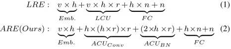
If we denote v, h, r, n to be the vocabulary size, word embedding size, region size and class number respectively (r= 2c+ 1), then the total number of parameters for (Qiao et al. 2018) and our method can be calculated as follows:

LRE: v×h

| {z } Emb.

+v×h×r

| {z } LCU

+h×n+n

| {z } F C

(1)

ARE(Ours) : v×h

| {z } Emb.

+h×(h×r)×r

| {z }

ACUConv

+ (2×h×r) | {z } ACUBN

+h×n+n

| {z } F C

(2)

For text classification task, especially large-scale datasets such as Yahoo Answers,vis several magnitudes’ larger than other hyperparameters likeh, r, n, and is the dominant factor of the total number of parameters.

(6)

Params (Qiao et al. 2018)’s Total

Ours Total LCU Only ACU Only

AG’s news 43,810,308 16,268,804 38,333,568 5,315,328 Sogou News 101,780,101 30,761,477 89,057,024 ∼

DBPedia 233,333,518 63,651,854 204,165,248 ∼

Yelp Review Polarity 118,065,410 34,832,130 103,307,008 ∼ Yelp Review Full 127,256,197 37,130,501 111,348,608 ∼ Yahoo! Answers 370,613,514 97,970,954 324,285,696 ∼ Amazon Review Polarity 403,850,498 106,278,402 353,368,960 ∼ Amazon Review Full 364,864,133 96,532,485 319,255,552 ∼

Table 3: Comparison of the number of parameters. ‘∼’ in the last column indicates that the number of parameters remains the same on different datasets. It is worth noting that these parameters correspond to the models that achieve the best performances where for (Qiao et al. 2018) region size and embedding size are 7 and 128, and for ours are 9 and 256 respectively.

澪澤澢澫

澪澧澢澩

澪澧澢澧

澪澥澢澧

澪澦澢澦

澪澤澢澪

澪澦澢澪

澪澨澢澧

澪澨澢澭

澪澩澢澨

澪澤澢澧澔

澪澦澢澩澔

澪澨澢澦澔

澪澩澢澤澔

澪澩澢澬澔

澪澤澢澥澔

澪澥澢澧澔

澪澨澢澤澔

澪澨澢澭澔

澪澥澢澫澔

澪澤澪澥澪澦澪澧澪澨澪澩澪澪澪澫

澺濕濧濨濨濙濬濨澜濉濢濝澝 澺濕濧濨濨濙濬濨澜澶濝澝 澷濂濂 激濆澹 澵濆澹澜濣濩濦濧澝

澵濗濗濩濦

濕濗濭

澜澙澝

澷濣濡濤濕濦濝濧濣濢澔濁濣濘濙濠濧 澥澤

澥澦澬 澦澩澪 澥澤澦澨

(a) (b)

澪澥澢澧

澪澨澢澨

澪澨澢澫 澪澨澢澭 澪澨澢澫 澪澨澢澩 澪澩

澪澥澢澪

澪澩澢澥 澪澩澢澦 澪澩澢澨

澪澩澢澫 澪澩澢澨

澪澥澪澦澪澧澪澨澪澩澪澪

澥澧澩澫澭澥澥

澵

濗濗濩

濦濕濗濭

澜澙

澝

濆濙濛濝濣濢澔濇濝濮濙

激濆澹 激濆澹澜濡濩濠澝 澵濆澹澜濣濩濦濧澝

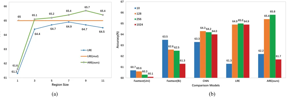
Figure 3: Effect of embedding size and region size. For (a) the embedding size is fixed to 128, and LRE(mul) refers to an ensemble of region sizes of [3,5,7], for (b) the region size is fixed to 7. All competitor results come from Qiao et al. (2018)’s paper.

architecture, and the last two columns indicate the parame-ters size that is used to generate the context unit, correspond-ing to the embeddcorrespond-ing look-up tensorU∈Rh×(2c+1)×v_and the meta-network respectively. From the table, we find that our total parameter space is only ˜26% large as that in Qiao et al. (2018), and if we only take the context unit generation part into account and leave out the rest, our ACU generation network reduced the LCU’s parameters’ number to less than 5%. It is worth to mention that if we choose the region and embedding size to be 7 and 128 as that in Qiao et al. (2018), the parameter space will be further reduced to nearly half of that in Table 3 and our method still outperforms Qiao et al. (2018)’s. Besides, our meta-network’s parameter space is invariant to the vocabulary size, making it possible to be applied in large-scale datasets with a large vocabulary size.

Effect of Embedding Size and Region Size

Apart from the main classification results, we also experi-ment with different embedding and region sizes and

com-pare with Qiao et al. (2018)’s method. The results from Fig-ure 3 show that our method outperforms LRE and its ensem-ble of multiple region sizes with significant margins. More-over, our method also performs better with different embed-ding sizes except for 1024, in which case the output space of thedynamically generated parametersis too large for the meta-network to learn. Besides, we find that the optimal re-gion and embedding size are different for ARE and LRE (9/256 and 7/128) which indicates our ARE requires a larger embedding size to contain more context information, and the meta-network is able to capture long-distance patterns, lead-ing to a larger optimal region size.

Visualization of Word Ambiguity Avoidance

In order to illustrate that our method is able to distinguish context-sensitive words, we select the two words like and

(7)

like well

positive

2.25 0.01 4.34 2.55 -0.67 5.30 1.99 2.58 10.34 2.72 5.13 2.80

neutral/negative

-5.30 -2.82 -3.20 -4.63 -3.53 -3.55 -3.42 -4.51 -2.81 -3.16 -1.82 -3.92

anyway I like the idea It arrived packaged Well and very promptly

didn't feel like the two main Well , what can I say

sentiment word

Figure 4: Heatmaps of Samples from Amazon Review Polarity. Green denotes positive contribution and red denotes negative. It demonstrates that our model is able to distinguish different meanings of the same word under different contexts.

strategy proposed in (Li et al. 2016) for visualization. The results are shown in Figure 4.

We find that in the first row, thelikeconveys the positive attitude in the sentenceI like the idea, its derivative is greater than other words, which means that it contributes most to the final prediction of positive, the wordwellmeansof high standard which also has positive effects on the classifica-tion result, thus corresponding to the highest value. In the second row, however, both words convey neutral or negative attitude, wherelikeis part of the phrasefeel likeandwellis a spoken expression, and the visualizations show that these two words do not contribute as much as that in the first row to the final sentiment prediction. These visualizations also accord with our intuition.

Choice of the Meta-network

It is worth noting that the choice of meta-network can be any differentiable architecture that is trainable using gradi-ent descgradi-ent. It can be multi-layer perceptron, convolutional network, or recurrent network etc. In this paper we choose a one-layer convolutional neural network to be our meta-network for its superior performance and simple meta-network structure.

In order to further investigate the influence of the choice of meta-network, we also experiment with the following variants:

• SmallCNN: Instead of producing ACU of size Kwi ∈ Rh×(2c+1)_{, the SmallCNN meta-network produces}

Kwi ∈ R

h×1_{, and uses the same set of filters for all the} positions from[−c: c]. This meta-network contains less parameters than our proposed CNN meta-network.

• FactoredCNN: The produced filters are Kwi ∈ R

u×1 whereuis relatively small compared toh. Then the fil-ters are transformed toK0 ∈ Rh×(2c+1)_{by multiplying} a matrixP ∈ Ru×(h×(2c+1))_{. This model can be} inter-preted as factorizing the filtersK0into the multiplication of two matrices:K0=KP, whereKis generated by the meta-network, andPis updated by gradient descent. This meta-network further reduces the number of parameters. In the experiment, we setu= 32.

• LSTM: We use an LSTM to generate the filtersKwhere the hidden unit of LSTM is of sizeh×(2c+ 1).

Hypernet AG DBP Yahoo.A.

CNN 93.1 99.1 74.9

SmallCNN 93.0 98.9 74.9

FactoredCNN 92.7 98.9 74.3

LSTM 92.5 98.6 73.5

GRU 92.5 98.6 73.5

Ensemble (CNN+LSTM) 93.1 99.1 75.1

Table 4: Impact of the Choice of the Meta-network

• GRU: We use a GRU to generate filtersKwhere the hid-den unit of LSTM is of sizeh×(2c+ 1).

• Ensemble (CNN+LSTM): We generate two set of fil-tersKCN N,KLST M, and use the element-wise product

KCN NKLST Mas the context unit.

We report the experimental results on AG’s News, DBPe-dia and Yahoo Answers dataset due to page limit. From the result we find that the recurrent structure is not so suitable for generating adaptive filters, where the CNN variants with smaller parameter space yield comparable performances.

Conclusion and Future Work

In this paper, we propose a novel region embedding method calledAdaptive Region Embeddingusing the meta-network structure which is able to adaptively capture regional com-positionality with a more compact parameter space. We also discuss the internal relationships between these methods un-der the Generalized Text Filtering framework, where our method corresponds to theinstance-level filteringwhich is more flexible. By experimenting on benchmark text classifi-cation datasets, we are able to gain higher classificlassifi-cation per-formances with a small parameter space, while also avoiding word ambiguity. In future, we aim to design more efficient structures of meta-network and combine techniques such as attention mechanism into our model.

Acknowledgments

(8)

References

Bertinetto, L.; Henriques, J. F.; Valmadre, J.; Torr, P.; and Vedaldi, A. 2016. Learning feed-forward one-shot learn-ers. InAdvances in Neural Information Processing Systems, 523–531.

Chen, J.; Qiu, X.; Liu, P.; and Huang, X. 2018. Meta multi-task learning for sequence modeling. InProceedings of the Thirty-Second AAAI Conference on Artificial Intelligence. Conneau, A.; Schwenk, H.; Barrault, L.; and Lecun, Y. 2017. Very deep convolutional networks for text classification. In

Proceedings of the 15th Conference of the European Chap-ter of the Association for Computational Linguistics: Vol-ume 1, Long Papers, volume 1, 1107–1116.

Fan, R.-E.; Chang, K.-W.; Hsieh, C.-J.; Wang, X.-R.; and Lin, C.-J. 2008. Liblinear: A library for large linear classifi-cation.Journal of machine learning research9(Aug):1871– 1874.

Forman, G. 2003. An extensive empirical study of feature selection metrics for text classification. Journal of machine learning research3(Mar):1289–1305.

Ha, D.; Dai, A. M.; and Le, Q. V. 2016. Hypernetworks. Ioffe, S., and Szegedy, C. 2015. Batch normalization: Accel-erating deep network training by reducing internal covariate shift. In International Conference on Machine Learning, 448–456.

Jia, X.; De Brabandere, B.; Tuytelaars, T.; and Gool, L. V. 2016. Dynamic filter networks. InAdvances in Neural In-formation Processing Systems, 667–675.

Joachims, T. 1999. Transductive inference for text classifi-cation using support vector machines. InICML, volume 99, 200–209.

Johnson, R., and Zhang, T. 2015a. Effective use of word order for text categorization with convolutional neural net-works. InProceedings of the 2015 Conference of the North American Chapter of the Association for Computational Linguistics: Human Language Technologies, 103–112. Johnson, R., and Zhang, T. 2015b. Semi-supervised con-volutional neural networks for text categorization via region embedding. InAdvances in neural information processing systems, 919–927.

Joulin, A.; Grave, E.; Bojanowski, P.; and Mikolov, T. 2017. Bag of tricks for efficient text classification. In Proceed-ings of the 15th Conference of the European Chapter of the Association for Computational Linguistics: Volume 2, Short Papers, volume 2, 427–431.

Kim, Y. 2014. Convolutional neural networks for sen-tence classification. In Proceedings of the 2014 Confer-ence on Empirical Methods in Natural Language Processing (EMNLP), 1746–1751.

Kingma, D. P., and Ba, J. 2014. Adam: A method for stochastic optimization.arXiv preprint arXiv:1412.6980. Li, L.; Jin, X.; Pan, S. J.; and Sun, J.-T. 2012. Multi-domain active learning for text classification. InProceedings of the 18th ACM SIGKDD international conference on Knowledge discovery and data mining, 1086–1094. ACM.

Li, J.; Chen, X.; Hovy, E. H.; and Jurafsky, D. 2016. Vi-sualizing and understanding neural models in nlp. In HLT-NAACL.

McCallum, A.; Nigam, K.; et al. 1998. A comparison of event models for naive bayes text classification. InAAAI-98 workshop on learning for text categorization, volume 752, 41–48. Citeseer.

Mikolov, T.; Sutskever, I.; Chen, K.; Corrado, G. S.; and Dean, J. 2013. Distributed representations of words and phrases and their compositionality. InNIPS.

Qiao, C.; Huang, B.; Niu, G.; Li, D.; Dong, D.; He, W.; Yu, D.; and Wu, H. 2018. A new method of region embed-ding for text classification. InInternational Conference on Learning Representations.

Shen, D.; Min, M. R.; Li, Y.; and Carin, L. 2018a. Learning context-aware convolutional filters for text processing. In

Proceedings of the 2018 Conference on Empirical Methods in Natural Language Processing, 1839–1848.

Shen, D.; Wang, G.; Wang, W.; Min, M. R.; Su, Q.; Zhang, Y.; Li, C.; Henao, R.; and Carin, L. 2018b. Baseline needs more love: On simple word-embedding-based models and associated pooling mechanisms. InACL.

Sundermeyer, M.; Schl¨uter, R.; and Ney, H. 2012. Lstm neu-ral networks for language modeling. InThirteenth Annual Conference of the International Speech Communication As-sociation.

Tang, D.; Qin, B.; and Liu, T. 2015. Document modeling with gated recurrent neural network for sentiment classifi-cation. InProceedings of the 2015 conference on empirical methods in natural language processing, 1422–1432. Wang, G.; Li, C.; Wang, W.; Zhang, Y.; Shen, D.; Zhang, X.; Henao, R.; and Carin, L. 2018. Joint embedding of words and labels for text classification. InACL.

Yang, Z.; Yang, D.; Dyer, C.; He, X.; Smola, A.; and Hovy, E. 2016. Hierarchical attention networks for document clas-sification. In Proceedings of the 2016 Conference of the North American Chapter of the Association for Computa-tional Linguistics: Human Language Technologies, 1480– 1489.