Spatial-Dynamic Externalities and Coordination in Invasive Species Control
Abstract. This paper investigates the coordination problem in transboundary species invasions. When invasions impact commodity markets and control decisions are made by many producers, a spatial externality arises due to market-level impacts such as reduced demand for commodities from invaded areas or the imposition of costly phytosanitary standards. Private control actions slow the invasion and alleviate these damages but are under-provided due to their public good nature. Industry trade groups and agricultural cooperatives become increasingly important for coordinating private control efforts at the market level. Unfortunately, there is limited research to guide these efforts. We show that the spread rate and the spatial configuration of producers are key factors when
determining the public benefits of private control decisions. To coordinate responses to invasions at the market level, a corrective mechanism is suggested in which invaded producers are compensated by all other producers for control actions that alleviate impacts to other producers.
Keywords: spatial-dynamic modeling; agricultural pests; phytosanitary standards; trade restrictions; agricultural cooperatives
1. Introduction
Invasive species cause tremendous losses in the US with several billions of dollars spent on decreasing their spread (Pimentel, 2011). Altering the spread of an established invader is a long-term balance between the flow of damages and relative control costs. This balance critically depends on the ecological and economic factors that dictate the evolution of the invasion and subsequent damages (Regev et al., 1976; Olson and Roy, 2008) and the interaction between regions, transmission pathways, and the availability of control measures such as inspection, removal, and restoration (Sanchirico et al., 2010).
Invasive species also impact large spatial areas requiring control actions by multiple affected individuals, e.g., land owners, regional governments, countries (Wilen, 2007). While invasive species control suffers from well-known problems of public good provision (Perrings et al., 2002), the problem is novel in that the supply of the public good (benefits of control that spillover to other individuals) is determined by 1) spatial-dynamic processes unique to each species and 2) the spatial configuration of decision makers. This paper integrates ecological and economic processes to study a spatial externality common in invasive species control decisions made by spatially-connected individuals.
Spatial externalities are likely when control efforts impact the movement of an invasive species across the landscape (Grimsrud et al., 2008; Rich et al. 2005a; Fenichel et al., 2013).1 A
negative externality is caused by the pattern of spread, such as the emigration of pests from high-density to low-high-density.2 A positive externality arises when benefits from individualistic control spillover to neighbors in the form of a decrease or delay of damages (Brown et al., 2002; Wilen, 2007). The fundamental reason for these externalities is that individual participants base control decisions on a subset of the total area at risk of invasion. Variable transfer payment agreements (Bhat and Huffaker, 2007), chained bilateral negotiation (Wilen, 2007), and Coasian exchange (Fenichel et al., 2013) have been suggested as ways to internalize these types of externalities.
Another positive externality centers on the deficiency of private efforts to ameliorate impacts to regional commodity markets. When an individual producer becomes invaded, that producer experiences a decline in profit due to 1) physical damage to the commodity which reduces yields and 2) impacts to the regional commodity market in the form of reduced demand for commodities from this region or the imposition of costly phytosanitary standards (Acquaye et al, 2005). While initially invaded producers fully internalize their physical damage when
making control decisions, they only incur a subset of the total economic impact to the regional market.3 This creates a tendency for individual producers to have control incentives that are not aligned with their neighbors (Cook et al., 2010).
For example, citrus canker was detected near Miami in 1995 (Gottwald et al., 2001). The USDA now believes that long-distance spread of the disease by hurricanes in 2004 and 2005
2 Bhat et al. (1993, 1996) show that multiple landowners necessitate a centralized control strategy which incorporates the effect of species diffusion on control. Rich et al. (2005b) find that regional control of foot and mouth disease (FMD) spread is diminished by spatial spillovers from neighboring regions which perform less control.
makes eradication infeasible and a new citrus canker management plan is being developed (Olson, 2006). Restrictions against the importation of citrus fruit from Florida have already had serious impacts on the state’s producers (Acquaye et al, 2005). If the bacterial agent that causes citrus canker becomes endemic to Florida, it will effectively result in prohibition of interstate commerce of fresh citrus fruit, which comprises approximately 20% of the State’s $8 billion commercial citrus industry (Muraro, 1986). Other highly susceptible cultivar such as grapefruit will become less economically viable due to requirements for multiple bacterial sprays (Gottwald et al., 2001). Individual orchard owners would only incur a portion of these market-level
impacts and would not consider how their control decisions would lessen market impacts on other orchard owners. On a more broad scale, countries may prohibit importation of citrus fruit from the United States due to the risk of invasion spreading to other states. Florida would only incur a portion of the impacts from a federal quarantine and would not consider how their control decisions would lessen market impacts on other citrus-producing states such as California.4
This paper joins the seminal work on barrier control of biological invasions (Sharov and Liebhold 1998; Sharov 2004) with the emerging literature on spatial-dynamic externalities to investigate market externalities that arise as an invasive species spreads across a landscape that is a source of supply for a regional commodity market.Following Sharov and Liebhold (1998), the model considers a biological invasion across a rectangular strip with control efforts focused in a barrier zone along the edge of the expanding population front. Increases in invaded area result in physical damage (lower yields, physical abnormalities) and market impacts. Market impacts
arise from 1) reduced demand for commodities from this region due to trade restrictions and quarantines or consumer perceptions of lowered commodity quality or 2) from the introduction of costly phytosanitary standards for exports from the regional market.
Unlike Sharov and Liebhold, the rectangular strip is managed by multiple producers such that individual producers make control decisions based only on a subset of the area at risk (i.e., their private property or jurisdictional considerations) and thus do not consider the full impact of the invasion on the local commodity market.5 Using the backward induction solution procedure proposed by Wilen (2007), we show that the shadow cost of an additional unit of invaded area is smaller for individual producers than it would be for the market as a whole. This implies that commodity markets which rely on a large number of small producers will support larger
invasions. If the market is comprised of producers of various sizes, invaded area will be larger if the species is introduced on a smaller producer and then spreads to larger producers.
We also identify the timing and sequence of Coase-like side-payments in which uninvaded and fully invaded individuals compensate individuals currently engaged in control for actions that slow the invasion and lessen impacts to the regional market as a whole. This series of side payments internalizes the spatial-dynamic externality and ensures each producer is better off under the series of side-payments thus soliciting voluntary participation by each producer. Such side-payments, organized by industry trade groups or cooperatives, become an attractive
approach for coordinating private invasive species control efforts in light of increasingly limited federal funds designated for invasive species control. These results expound on many of the
5
concepts and ideas in Wilen (2007) and Epanchin-Niell and Wilen (2014) and break new ground by considering market level impacts, accelerating rates of spread, and the effect of parcel size and location on biological invasions.
2. Modeling a Species Invasion
For convenience, the definition of each variable and parameter in the model is summarized in Table 1. Following Sharov and Liebhold (1998), a regional commodity market is supplied by a rectangular strip whose width is normalized to one.6 This rectangular strip is divided into I individually owned parcels of land, labeled as 1 to I from west to east (see Figure 1). Let Ai
represent the size of the parcel owned by producer i = 1, 2,…,I and 𝐴 = ∑𝐼𝑖=1𝐴𝑖 reflect the size of the region. The species is introduced on parcel 1 and spreads from west to east along the length of the rectangle. Cumulative distance spread at time t is given by 𝑥(𝑡) with 𝑥0
representing the distance spread when the invasion was first detected at 𝑡0 = 0. Each parcel is either “not invaded” (the invasion front has not yet reached the western border of the parcel), “being invaded” (the invasion front has reached and is spreading within the parcel), or “fully invaded” (the invasive species has fully spread across the parcel).
The spread of an invasive species is “a process by which the species expands its range from a habitat in which it currently occupies to one in which it does not” and there are two
processes (Liebhold and Tobin, 2008). Local or short-range dispersal due to the growth of the population is characterized by a constant spread rate. In contrast, long-distance dispersal such as
human-mediated or wind dispersal results in isolated colonies, which grow and eventually merge into the main population of invasive species. The combination of the two processes (known as stratified dispersal) causes spread to accelerate over time (Liebhold and Tobin, 2008). Let the spread of the invasion be given by 𝑥̇ = 𝑔𝑥(𝑡) where 𝑔 > 0 is the intrinsic spread rate
of the invasive species. Here we assume no new introductions and an exponentially increasing invaded area which is consistent with a combination of short and long range dispersal.7
Economic damages due to invasion in the region have a physical and market component. Physical damages refer to the pecuniary losses due to crop death or product decline. For example, the rice water weevil causes an average yield loss of 7% ($64.05 /acre) in the US (Hummel, 2009) and 10%-20% in the province of Hebei, north of China (Yu et al., 2008). Market damage results from price effects, restricted markets, and the imposition of costly phytosanitary standards. Consumers may consider commodities from an invaded region as damaged goods resulting in lower demand. Demand may also be reduced due to quarantines or trade restrictions intended to prevent new introductions outside the regional market. These market damages occur throughout the region since consumers and regulators will rarely be able to distinguish between commodities from invaded and non-invaded parcels within an invaded region.
The physical and market damages are shown in Figure 2. Once the region becomes invaded, physical commodity damage on invaded parcels causes the supply curve to shift from S0 to S1 and quantity supplied falls from Q0 to Q1. Typical of many small regional commodity markets, demand facing producers is perfectly elastic such that only producers are affected by this
reduction in supply. If phytosanitary measures are required in the regional market, the marginal cost of production for both invaded and non-invaded producers will increase and the quantity supplied will be reduced further to Q2. If consumers perceive commodities from the regional market as inferior or if access to export markets is restricted, commodities from the invaded region will receive a lower price further impacting regional producers.
An individual producer’s damage function captures these physical and market damages at
each stage of the invasion. When a parcel is uninvaded, that producer only experiences market damages. To provide a general framework that accommodates both shifts in supply (costly phytosanitary measures) and demand (restricted markets), market dynamics are lumped into a parcel-level market damage function, 𝐷𝑖𝑚, that adjusts instantaneously to the extent of the invasion.8 When a parcel is currently being invaded or is fully invaded, that producer
experiences both market damages and physical damages 𝐷𝑖𝑝. This implies that an individual’s total damage is a function of both the size of the invasion and the size of the individual
producer’s parcel: 𝐷𝑖𝑚+ 𝐷
𝑖𝑝 = 𝐷𝑖[𝑥(𝑡), 𝐴𝑖] > 0. As the invasion grows, market impacts felt by
the individual producer increase due to more restricted market access or more stringent
phytosanitary standards (∂𝐷𝑖⁄𝜕𝑥 > 0); however, the marginal market impacts may diminish as the invasion progresses (∂2𝐷𝑖⁄𝜕𝑥2 ≤ 0).9 The total damage to all producers in the regional
market is defined as 𝐷[𝑥(𝑡), 𝐴] = ∑𝐼𝑖=1𝐷𝑖[𝑥(𝑡), 𝐴𝑖].10
8 Using a lumped damage function also allows market damages to be reinterpreted as other spatial-dynamic
externalities. For example, market damages may be roughly equivalent to damage arising from a simplified form of biological spillover (dispersal) where biomass distributes uniformly across the landscape in proportion to the current invasion extent.
A control action is available to producers which will reduce the rate of spread across their parcel from 𝑔 to [𝑔 − 𝑢𝑖(𝑡)] where 0 ≤ 𝑢𝑖 ≤ 𝑢̅ is the reduction in the spread rate due to control by producer i at time 𝑡 and 𝑢̅ is the maximum control rate available. Control efforts slow spread if 𝑢𝑖(𝑡) < 𝑔, reverse spread if 𝑢𝑖 > 𝑔, and stop spread if 𝑢𝑖 = 𝑔. Efforts to control spread are
focused in a barrier zone along the edge of the expanding population front (Sharov and Liebhold, 1998), so producers can take control actions only when their parcel is being invaded. Once the invasion spreads from parcel i to a neighboring parcel, producer i stops control and the
neighboring producer starts spread control.11 In this way, the individual spread control process is akin to a relay. In this barrier control setting, the cost of spread control is determined by the control rate 𝑐[𝑢𝑖(𝑡)] with 𝜕𝑐 𝜕𝑢⁄ 𝑖 > 0 and 𝜕2𝑐 𝜕𝑢⁄ 𝑖2 > 0.12
In what follows we first characterize the collective control decision from the perspective of all producers in the regional market. We then illustrate the spatial externality by contrasting the collective decision with that of the private control decisions of each individual producer.
3. Collective Control by all Regional Producers
response. Such concave damage functions have been noted in the pollution control literature (Baumol 1964; Starrett 1972).
10
Invasive species spread may also cause significant environmental damage such as reduction in biodiversity and native species extinction. Due to the paper’s focus on spatial externalities in commodity markets, we abstract from these impacts. As a result, D should not be interpreted as a measure of social damages from invasion.
11
This assumption only applies to control actions that alter the spread of the invasion and does not preclude the possibility that producers may continue population-related control actions once fully invaded. Due to the paper’s focus on externalities between neighbors, we have chosen to simplify the model by focusing only on control actions that alter the spread of the invasion.
12 Control costs may also be a function of 𝐴
𝑖 which would change the degree of control chosen on a particular parcel.
The collective control strategy 𝑢(𝑡) represents the decisions of a coordinated control effort by all producers. Such coordinated efforts would reflect the control decisions of an industry trade group or agricultural cooperative. For example, a cooperative of ranchers was created to share costs and coordinate efforts to control knapweed in Montana (Fiege, 2005) and yellow starthistle in California (Epanchin-Niell et al., 2010). The objective of a collective control strategy is to choose 𝑢(𝑡) to minimize the total damages and control costs across the region
(1) max
𝑢(𝑡) ∫ {𝑅(𝐴) − 𝐷[𝑥(𝑡), 𝐴] − 𝑐[𝑢(𝑡)]}𝑒 −𝑟𝑡𝑑𝑡 ∞
0
subject to 𝑥̇ = [𝑔 − 𝑢(𝑡)]𝑥(𝑡), 𝑥(0) = 𝑥𝑜> 0, and 0 ≤ 𝑢 ≤ 𝑢̅ where 𝑅(𝐴) is the agricultural
revenue earned in the entire region before invasion, and r is the discount rate. There are two cases for the terminal condition. The first case is preservation of a portion of the region leading to a steady-state invaded area that is smaller than the region.13 The second case finds the region being fully invaded such that the terminal condition is equal to the size of the region.
The current value Hamiltonian for this problem is
(2) 𝐻[𝑢(𝑡), 𝑥(𝑡), 𝜔(𝑡)] = {𝑅(𝐴) − 𝐷[𝑥(𝑡), 𝐴] − 𝑐[𝑢(𝑡)]} + 𝜔(𝑡)[𝑔 − 𝑢(𝑡)]𝑥(𝑡)
where 𝜔 < 0 is the current value costate variable.14 The costate variable represents the shadow cost of an incremental increase in invaded area (or the marginal value of uninvaded land). The corresponding necessary conditions for an interior solution are15
13
Introducing invasive species control by reducing the spread rate introduces a stock dependence in the control decision that makes complete eradication economically infeasible. However, it is possible to consider complete eradication in our model by assuming the invasion is eradicated from the region when it reaches a very small value: 𝑥𝑚𝑖𝑛. Complete eradication from the region is akin to a steady state smaller than 𝑥𝑚𝑖𝑛. We note this feature of the
model but proceed with the two more common cases of full invasion and local suppression.
14 The constraints on the control variable are imposed using Lagrangian multipliers but are omitted for notational simplicity.
(3) −𝜔∗(𝑡)𝑥∗(𝑡) −𝜕𝑐(𝑢
∗)
𝜕𝑢 = 0
(4) 𝜔̇ = [𝑟 − (𝑔 − 𝑢∗ ∗(𝑡))]𝜔∗(𝑡) +𝜕𝐷(𝑥
∗,𝐴)
𝜕𝑥
(5) 𝑥∗̇ = [𝑔 − 𝑢∗(𝑡)]𝑥∗(𝑡)
where 𝑢∗(𝑡) and 𝑥∗(𝑡) designates optimal control and invaded area under collective control, and
𝜔∗(𝑡) represents the shadow cost of additional invaded area from the perspective of the
collective. From (3), the optimal control rate is adjusted to ensure the marginal control cost equals the incremental damage of invaded area: 𝜕𝑐(𝑢∗) 𝜕𝑢⁄ = −𝜔∗(𝑡)𝑥∗(𝑡). If −𝜔∗(𝑡)𝑥∗(𝑡) >
𝜕𝑐(𝑢∗) 𝜕𝑢⁄ , control is implemented to the maximum degree. No control is optimal if the
incremental damage is lower than the marginal control cost: −𝜔∗(𝑡)𝑥∗(𝑡) < 𝜕𝑐(𝑢∗) 𝜕𝑢⁄ . If this condition holds at every point of invasion, the damage caused by the invasion is ignored and the invasion spreads at its natural rate across the region. The optimal collective control strategy
implies different outcomes on each parcel. With initial invaded area ∑𝑖−1𝑗=1𝐴𝑗, parcel i becomes
fully invaded under the social optimum when 𝜕𝑐(𝑔)𝜕𝑢 > −𝜔∗(𝑡) ∑𝑖𝑗=1𝐴𝑗 and the invasion will be
eradicated on parcel i under the social optimum when 𝜕𝑐(𝑔)𝜕𝑢 < −𝜔∗(𝑡) ∑𝑖−1𝑗=1𝐴𝑗.
Solving equation (3) for 𝜔∗(𝑡), taking the time derivative and using (5) yields
(6) 𝜔̇ = −∗
𝜕2𝑐(𝑢∗) 𝜕𝑢2
𝑑𝑢(𝑡)
𝑑𝑡 −[𝑔−𝑢∗(𝑡)] 𝜕𝑐(𝑢∗)
𝜕𝑢
𝑥∗(𝑡)
Substituting (6) into (4), and using (3) and (5)
(7) 𝑢∗̇ = 𝑟
𝜕𝑐(𝑢∗) 𝜕𝑢 −
𝜕𝐷(𝑥∗,𝐴) 𝜕𝑥 𝑥∗(𝑡) 𝜕2𝑐(𝑢∗)
𝜕𝑢2
= 𝑟
𝜕𝑐(𝑢∗)
𝜕𝑢 −{∑𝐼𝑖=1𝜕𝐷𝑖[𝑥∗(𝑡),𝐴𝑖]𝜕𝑥 }𝑥∗(𝑡) 𝜕2𝑐(𝑢∗)
𝜕𝑢2
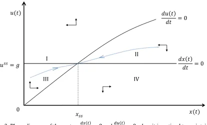
Figure 3 presents a phase diagram of this system when it is optimal to maintain a portion of the region as uninvaded (case 1).16 Provided the curvature of the damage function is not too
severe (0 ≥ 𝜕
2𝐷
𝜕𝑥2 >
−𝜕𝐷 𝜕𝑥⁄
𝑥 ), the slope of the 𝑢̇ = 0 isocline is positive reflecting the desire for
more control in response to larger damages. The 𝑥̇ = 0 isocline is realized by equating 𝑢∗(𝑡) and the invasive species natural spread rate. The steady state invaded area is solved directly from
equations (5) and (7) and is implicitly defined by 𝑥𝑠𝑠 = 𝑟𝜕𝐷 𝜕𝑥𝜕𝑐 𝜕𝑢⁄⁄ . Off- equilibrium conditions
suggest a saddle-point stable trajectory, indicated by the dotted line in isosectors II and III. Isosectors I and IV represent non-optimal trajectories. If marginal damage declines rapidly as
the invasion progresses (𝜕
2𝐷
𝜕𝑥2 <
−𝜕𝐷 𝜕𝑥⁄
𝑥 ), the slope of the 𝑢̇ = 0 isocline is negative. Here it is
optimal to allow the region to become fully invaded (case 2).
4. Individual Control Relay
Invasive species control becomes the responsibility of individual producers in the absence of an organization or institution that represents the interest of the regional market. Individual control falls short of collective control because control actions involve private costs but partially public benefits. Individual producers will first suffer market damage before their parcel is invaded since market damages impact all producers in an invaded region. When the invasion spreads onto a new parcel, that producer also begins to experience physical damage (which reaches a maximum when their parcel is fully invaded) and chooses a level of control at each point in time to minimize the present value of her own individual damage and control cost flow
into perpetuity. Once the invasion spreads to other parcels, she will stop control since her control efforts no longer alter the spread of the invasion. However, she continues to experience market damage (which increases as the invasion spreads to other parcels) and a constant amount of physical damage.
Each producer’s control strategy is one turn of an individual spatial control relay. The invasive species is first discovered on parcel 1 at 𝜏0 which signifies the start of the individual control relay. For i > 1, 𝜏𝑖−1 is the time at which parcel i-1 becomes fully invaded. This also represents the time the invasion initially occurs on parcel 𝑖 signifying a transfer in the individual control relay.
The nature of the control relay limits the degree of strategic behavior on the part of individual producers. Control decisions made by previously invaded producers determine the time subsequent producers become invaded but do not influence subsequent control decisions. In contrast, a currently invaded producer must anticipate the control decisions of subsequently invaded individuals. This allows the private optimum control strategy to be treated as a chain of individually optimal control problems solved through backward induction. Links between individual control problems are handled through initial conditions and terminal salvage values. The salvage value represents an individual’s anticipation of future damages given all subsequent
individuals behave optimally. The optimal control path of the last individual in the region or the individual that stops spread (the steady state individual) determines the terminal salvage value of the preceding individual’s control problem. This procedure is repeated to find the optimal control
Assume the individual control relay results in a positive steady-state (𝑥𝑛𝑠𝑠) being reached within parcel 𝑛 ∈ [1, 𝐼] at time 𝜏𝑛𝑠𝑠.17 Producer n is facing an infinite horizon optimal control problem since control must be exerted indefinitely to keep the invasion at steady state. When the invasion reaches the west border of her parcel, producer n solves
(8) max
𝑢𝑛(𝑡) ∫ {𝑅(𝐴𝑛) − 𝐷𝑛[𝑥(𝑡), 𝐴𝑛] − 𝑐[𝑢𝑛(𝑡)]}𝑒 −𝑟𝑡𝑑𝑡 ∞
𝜏𝑛−1
subject to 𝑥̇ = [𝑔 − 𝑢𝑛(𝑡)]𝑥(𝑡), 𝑢𝑛(𝑡) ≥ 0, and initial condition
𝑥(𝜏𝑛−1) = {
𝑥𝑜 𝑛 = 1
∑𝑛−1𝑗=1𝐴𝑗 𝑛 > 1 .
The current value Hamiltonian for the control path on parcel n is
(9) 𝐻𝑛 = {𝑅(𝐴𝑛) − 𝐷𝑛[𝑥(𝑡), 𝐴𝑛] − 𝑐[𝑢𝑛(𝑡)]} + 𝜔𝑛(𝑡)[𝑔 − 𝑢𝑛(𝑡)]𝑥(𝑡)
where 𝜔𝑛(𝑡) < 0 is the current value costate variable associated with invaded area on parcel n. The corresponding current value necessary conditions can be written as
(10) −𝜕𝑐(𝑢𝑛
′)
𝜕𝑢𝑛 − 𝜔𝑛
′(𝑡)𝑥′(𝑡) = 0
(11) 𝜔̇𝑛′ = [𝑟 − (𝑔 − 𝑢𝑛′(𝑡))]𝜔𝑛′(𝑡) +𝜕𝐷𝑛(𝑥 ′,𝐴
𝑛) 𝜕𝑥
(12) 𝑥̇′= [𝑔 − 𝑢𝑛′(𝑡)]𝑥′(𝑡)
where 𝑢𝑛′ designates optimal control by producer n, 𝑥′(𝑡) the optimal invaded area under the individual control relay, and 𝜔𝑛′(𝑡) the shadow cost of additional invaded area from producer n’s perspective. From (10), the optimal control rate is adjusted to ensure the marginal control cost equals the incremental damage of invaded area: 𝜕𝑐(𝑢𝑛′) 𝜕𝑢⁄ 𝑛 = −𝜔𝑛′(𝑡)𝑥′(𝑡). If
−𝜔𝑛′(𝑡)𝑥′(𝑡) > 𝜕𝑐(𝑢
𝑛′) 𝜕𝑢⁄ 𝑛, control is implemented to the maximum degree. No control is
optimal if the incremental damage is lower than the marginal control cost: −𝜔𝑛′(𝑡)𝑥′(𝑡) <
𝜕𝑐(𝑢𝑛′) 𝜕𝑢 𝑛
⁄ . If this condition holds at every point of invasion, the damage caused by the
invasion is ignored under and the invasion spreads at its natural rate across the region. With an initial invaded area ∑𝑖−1𝑗=1𝐴𝑗, parcel i becomes fully invaded under the individual optimum when
𝜕𝑐(𝑔)
𝜕𝑢𝑖 > −𝜔𝑖
′(𝑡) ∑ 𝐴 𝑗 𝑖
𝑗=1 and will eradicate a positive initial invasion under the individual
optimum when 𝜕𝑐(𝑔)𝜕𝑢
1 < −𝜔1
′(𝑡) ∑ 𝐴 𝑗 𝑖−1
𝑗=1 . Following the series of substitutions outlined in section
3, producer 𝑛’s optimized dynamic system is described by equation (12) and
(13) 𝑢̇𝑛′ = 𝑟
𝜕𝑐(𝑢𝑛′)
𝜕𝑢𝑛 −𝜕𝐷𝑛(𝑥′,𝐴𝑛)𝜕𝑥 𝑥′(𝑡) 𝜕2𝑐(𝑢𝑛′)
𝜕𝑢𝑛2
Now let’s turn our attention to the control decisions of all previously invaded producers
denoted as 𝑞 ∈ [1, 𝑛 − 1]. Unlike parcel n, the control problem on parcel q is characterized by a free terminal time 𝜏𝑞 < 𝜏𝑛𝑠𝑠 and free terminal state 𝑥(𝜏𝑞) ≤ ∑𝑞𝑗=1𝐴𝑗 since control actions alter
the rate of spread across the parcel. Individual q solves
(14) max𝑢𝑞(𝑡) ∫ {𝑅(𝐴𝑞) − 𝐷𝑞[𝑥(𝑡), 𝐴𝑞] − 𝑐[𝑢𝑞(𝑡)]}𝑒−𝑟𝑡𝑑𝑡
𝜏𝑞
𝜏𝑞−1 + 𝑒
−𝑟𝜏𝑞𝑠𝑞[𝑥(𝜏𝑞)]
subject to 𝑥̇ = [𝑔 − 𝑢𝑞(𝑡)]𝑥(𝑡), 𝑢𝑞(𝑡) ≥ 0, initial condition
𝑥(𝜏𝑞−1) = {∑𝑥𝑜 𝑞 = 1𝐴
𝑗 𝑞−1
𝑗=1 𝑞 > 1
with 𝜏𝑞−1 given. 𝑠𝑞[𝑥(𝜏𝑞)] is a salvage value and represents the present value damage suffered
by producer q after becoming fully invaded (𝜏𝑞 to ∞)
(15) 𝑠𝑞(𝑥(𝜏𝑞)) = ∫ −𝐷𝜏𝑞 𝑞[𝑥(𝑡), 𝐴𝑞]
𝑠𝑠
0 𝑒−𝑟𝑡𝑑𝑡 +
where 𝜏𝑞𝑠𝑠 = 𝜏𝑛𝑠𝑠 − 𝜏𝑞 represents the time between individual q becoming fully invaded and the
individual control relay reaching the steady state. The first term in (15) captures the present value of increasing market damages (and constant production damages) that accrue to producer q after being fully invaded but before the individual control steady state is reached. The second term captures the constant flow of physical and market damages that accrue to producer q after the steady state invaded area is reached. Producer q takes the control decisions of all subsequently invaded producers as given when evaluating 𝑠𝑞.
From (14), the current value necessary conditions can be written as
(16) −𝜕𝑐(𝑢𝑞
′)
𝜕𝑢𝑞 − 𝜔𝑞
′(𝑡)𝑥′(𝑡) = 0
(17) 𝜔̇𝑞′ = [𝑟 − (𝑔 − 𝑢𝑞′(𝑡))] 𝜔𝑞′(𝑡) +𝜕𝐷𝑞(𝑥
′,𝐴 𝑞) 𝜕𝑥
(18) 𝑥̇′ = [𝑔 − 𝑢𝑞′(𝑡)]𝑥′(𝑡)
The current value transversality condition for 𝜏𝑞 is
(19) 𝑅(𝐴𝑞) − 𝐷𝑞[𝑥′(𝜏𝑞), 𝐴𝑞] − 𝑐[𝑢𝑞′(𝜏𝑞)] + 𝜔𝑞′(𝜏𝑞)𝑥̇′(𝜏𝑞) = 𝑟𝑠𝑞[𝑥(𝜏𝑞)]
which states that the optimal choice for 𝜏𝑞 should equate the marginal cost of a longer time horizon (left-hand side) with the marginal benefit of delaying the salvage value (right-hand side).
The current value transversality condition for 𝑥(𝜏𝑞) is given by the complementary slackness
condition [∑𝑞𝑗=1𝐴𝑗 − 𝑥(𝜏𝑞)]𝜔𝑞𝑒−𝑟𝜏𝑞 = 0. In order for parcel n to be the steady state parcel,
∑𝑞𝑗=1𝐴𝑗 = 𝑥′(𝜏
𝑞) must hold for all q which allows for 𝜔𝑞′𝑒−𝑟𝜏𝑞 ≤ 0.
(20) 𝑢̇𝑞′ =
𝑟𝜕𝑐(𝑢𝑞′) 𝜕𝑢𝑞 −
𝜕𝐷𝑞(𝑥′,𝐴𝑞) 𝜕𝑥 𝑥′(𝑡) 𝜕2𝑐(𝑢𝑞′)
𝜕𝑢𝑞2
The optimal dynamic system for producer n and producer q is the same as the collective system except for 𝜕𝐷𝑛(∙′) 𝜕𝑥⁄ < 𝜕𝐷(∙′) 𝜕𝑥⁄ and 𝜕𝐷𝑞(∙′) 𝜕𝑥⁄ < 𝜕𝐷(∙′) 𝜕𝑥⁄ . This implies the individual
producer’s optimal control path on each parcel will be lower than the collective control path.18
From (13) and (20), the individual isocline 𝑢̇𝑖 = 0 is underneath the collective isocline 𝑢̇ = 0. As a result of this lower level of control, the steady state invaded area under individual control is larger than under the collective control process.
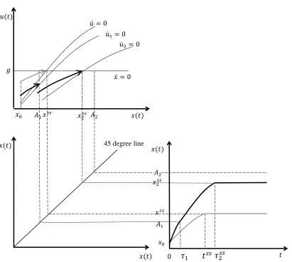
To illustrate these findings, consider the hypothetical scenario in Figure 4 where an initial invaded area of size 𝑥0 is discovered at 𝑡0 = 0. The individual isoclines 𝑢̇1 = 0 and 𝑢̇2 = 0 are always under the collective isocline 𝑢̇ = 0 and the individual control rate at a given invasion area is smaller than the collective one, 𝑢1′(𝑥) ≤ 𝑢∗(𝑥) and 𝑢2′(𝑥) ≤ 𝑢∗(𝑥). This gap between the individual and collective control rate shrinks as the size of the individual parcel 𝐴𝑞 approaches
the size of the total area at risk 𝐴. Because the individual’s optimal control rate is lower than the collective one for a given invaded area before the steady-state, the invasion is spreading faster under individual control than under collective control. At time 𝜏1, parcel 1 is fully invaded, then the owner of parcel 2 starts her control and reaches the steady state 𝑥2𝑠𝑠 at time 𝜏2𝑠𝑠. The steady
state invaded area under collective optimal control is smaller and reached sooner at time 𝑡𝑠𝑠. Comparative dynamics reveal that the discrepency between invasion outcomes under individual and collective control declines as the size of the individual parcel grows. From (20),
𝑢̇𝑞′ = 0 only when 𝑟𝜕𝑐(𝑢𝑞 ′)
𝜕𝑢𝑞 −
𝜕𝐷𝑞(𝑥′,𝐴𝑞)
𝜕𝑥 𝑥
′(𝑡) = 0. Using the implicit function theorem and
assuming the marginal damage from invasion increases as parcel size increases, 𝜕𝑢𝑞𝜕𝐴
𝑞=
𝜕2𝐷𝑞(𝑥′,𝐴𝑞) 𝜕𝑥𝜕𝐴𝑞 𝑥(𝑡)
𝑟𝜕2𝑐(𝑢𝑞′) 𝜕𝑢𝑞2
> 0. This has three important implications for the deficiency of individual control
of a spreading invader.19 First, commodity markets which rely on a large number of producers with small spatial holdings will support larger invasions. Second, the total invaded area will be larger if the species is introduced on a smaller producer and then spreads to larger producers. If the invasion starts on a relatively large parcel, fewer benefits of control are ignored by the individual producer early in the invasion when the area at risk of invasion is at its largest. Third, spatial considerations influence the benefits of collective action. The magnitude of the inefficiency generated by individual action will be small with a small number of producers each managing a large portion of the area at risk.
5. Side Payments to Induce Coordination
The deficiency of individual control is due to the mismatch between market-level invasion impacts and the limited spatial consideration of the individual producer. Specifically, producer i is only concerned with her private benefits of control, thus excluding the public or market-level benefits to neighboring producers when making her optimal control decision. Thus, a central management authority representing the regional market always has an incentive to encourage producer i to enact more control. Side payments between producers could be organized by a
regional agricultural cooperative or market interest group to motivate individual producers to compensate other producers for the public or market-level benefits of their control actions. When a producer is currently being invaded and making control decisions, she receives a side payment; and when a producer is fully invaded or uninvaded, she makes side payments to the producer currently engaged in control.
The side payment has two objectives. First, internalize the external market damages and the delay in physical damage and control cost enjoyed by all subsequently invaded producers. However, collective control creates winners and losers suggesting that all individuals will not choose to participate in the collective control strategy at each point in time. The second objective of the side payment is to ensure voluntary participation by making each individual no worse off following the series of side payments. Individual producers will bargain ex ante to decide how the winners from collective control will compensate the losers. The boundary of the bargaining space will be defined by the winner’s maximum willingness to pay (WTP) for the collective control strategy and the loser’s minimum willingness to accept (WTA). Winners will not choose
to participate in the side-payment program if they are required to pay more than their WTP and losers will not choose to participate if they receive a payment less than their WTA. For
exposition, we assume the side payment is equal to the total WTP for collective control.20 Unlike the variable transfer payment of Bhat and Huffaker (2007), the bargaining strengths of participants do not change since producers are invaded and engage in control sequentially. This
20
rules out strategic behavior and ensures our ex ante schedule of side payments is sufficient to ensure continued compliance as the invasion unfolds.
Producer i is currently being invaded and engaging in control. Since producer i is currently controlling spread, she receives a side payment. While this payment is organized and carried out by a central management authority, it is funded by all other producers who benefit from producer i’s control efforts −𝑖 ≠ 𝑖. Due to the presence of avoided market damages,
physical damage, and control cost, both fully invaded and uninvaded producers are willing to pay producer i for additional control. Producers who are not invaded even with the individualistic control relay are not willing to make any contributions toward collective action. The willingness to pay for collective action by all other producers is equal to the damages and control costs avoided through collective control. The side payment offered by producer -i to producer i when the invasion is of size x(t) is
(21) 𝐹−𝑖→𝑖(𝑡) = { 𝐷−𝑖
𝑚(𝑥′, 𝐴
−𝑖) − 𝐷−𝑖𝑚(𝑥, 𝐴−𝑖) 𝑖𝑓 − 𝑖 < 𝑖
𝐷−𝑖(𝑥′, 𝐴
−𝑖) − 𝐷−𝑖(𝑥, 𝐴−𝑖) + c(𝑢−𝑖′ ) 𝑖𝑓 𝑖 < −𝑖 ≤ 𝑛
The total side payment offered to producer i is (22) 𝑆𝑃𝑖(𝑡) = ∑𝐼−𝑖=1 𝐹−𝑖→𝑖(𝑡)
−𝑖≠𝑖 = ∑ [𝐷−𝑖(𝑥
′, 𝐴
−𝑖) − 𝐷−𝑖(𝑥, 𝐴−𝑖) + c(𝑢−𝑖′ )] 𝐼
−𝑖=1 −𝑖≠𝑖
expended by other producers under individual control. Voluntary participation in the side payment program occurs provided the total willingness to pay for collective action exceeds producer i's willingness to accept for the additional control under collective action:
(23) ∫ 𝑒−𝑟𝑡{[𝑐(𝑢𝑖∗) − 𝑐(𝑢𝑖′)] − [𝐷𝑖(𝑥′) − 𝐷𝑖(𝑥∗)]}𝑑𝑡 ≤ ∫ 𝑒−𝑟𝑡𝑆𝑃𝑖(𝑡) 𝑑𝑡
By increasing her control rate, producer i lowers 𝑥 at a point in time. This increases the side payment producer i receives in two ways. First, it reduces the market damages experienced by others which increases the difference between 𝐷−𝑖(𝑥′, 𝐴−𝑖) and 𝐷−𝑖(𝑥, 𝐴−𝑖). Second it increases 𝜏𝑖 to 𝜏𝑖𝑠 which allows producer i to receive a side payment for a longer period of time.
The difference between 𝐷−𝑖(𝑥′, 𝐴−𝑖) and 𝐷−𝑖(𝑥, 𝐴−𝑖) from 𝜏𝑖 to 𝜏𝑖𝑠 captures the delay in physical damages while c(𝑢−𝑖′ ) > 0 captures the control expenditures that would have been expended by other producers with the more rapid invasion.
Assume the invasion has yet to reach the steady-state parcel n. Let 𝑢𝑞𝑠(𝑡) represent
individual 𝑞’s reduction in the invasive species spread rate in response to this series of side payments from all other producers. The producer on parcel 𝑞 solves
(24) max
𝑢𝑞𝑠(𝑡) ∫
{𝑅(𝐴𝑞) − 𝐷𝑞[𝑥, 𝐴𝑞] − 𝑐[𝑢𝑞𝑠] + 𝑆𝑃
𝑞}𝑒−𝑟𝑡𝑑𝑡 𝜏𝑞
𝜏𝑞−1 + 𝑒
−𝑟𝜏𝑞𝑠
𝑞[𝑥(𝜏𝑞)]
subject to 𝑑𝑥 𝑑𝑡⁄ , all relevant initial and terminal conditions and
𝑠𝑞(𝑥(𝜏𝑞)) = ∫ {−𝐷𝜏𝑞 𝑞[𝑥(𝑡), 𝐴𝑞] − 𝐹𝑞→𝑖(𝑡)} 𝑠𝑠
0 𝑒−𝑟𝑡𝑑𝑡 +
[−𝐷𝑞(𝑥𝑛𝑠𝑠,𝐴𝑞)−𝐹𝑞→𝑛(𝜏𝑛𝑠𝑠)]𝑒−𝑟𝜏𝑞𝑠𝑠 𝑟
compatible after q becomes fully invaded. The producer on steady-state parcel n makes side payments to all other producers before becoming invaded. Eventually parcel n becomes invaded and producer n solves
(25) max
𝑢𝑛𝑠(𝑡) ∫ {𝑅(𝐴𝑛) − 𝐷𝑛[𝑥(𝑡), 𝐴𝑛] − 𝑐[𝑢𝑛
𝑠(𝑡)] + 𝑆𝑃
𝑛}𝑒−𝑟𝑡𝑑𝑡 ∞
𝜏𝑛−1
Because she must engage in perpetual control to keep the invasion at steady state, producer n receives a continuous stream of side payments from other producers to preserve the remaining un-invaded area and prevent any additional market-level damages.
6. Conclusion
This paper develops a spatial-dynamic control model to synthesize the biological and economic properties of invasive species, such as the spread process, damage and control cost, and individual control by multiple spatially-connected producers in a regional commodity market being invaded. This outcome is due to the presence of market-level impacts from invasions such as trade restrictions, reduced demand for regional commodities, or costly phytosanitary
requirements. Reductions in these impacts are treated as public benefits by individual producers engaged in invasive species control. Although individual producers consider physical
First, commodity markets which rely on a large number of small producers will support larger invasions. Relying on individual producers to control the spread of an invasion will be problematic in a highly competitive regional commodity market. This suggests that the trend from small to large farms may actually help contain invasive species that damage crops which are typically characterized by large monetary damages. This is consistent with Hansen and Libecap’s (2004) study of the Dust Bowl which reveals that the abundance of small farms in the 1930s compromised the control of wind erosion. The limited scale of small farmers encouraged less erosion control than larger farmers increasing the amount of sand blown to leeward farms. The collective control necessitated the establishment of soil conservation districts and improved the coordination of farmer’s erosion control. In the same way, the number and size of
participants will also influence invasive species control.
Second, if the market is comprised of producers of various sizes, the order of invasion becomes an important factor in determining the ultimate size of the invasion. Specifically, the invaded area will be larger if the species is introduced on a smaller producer and then spreads to larger producers. This suggests that the location of the initial invasion with respect to political boundaries (individual property lines, state borders) is a key determinate of the eventual size of an invasion.
coordinate invasive species control efforts requires balancing the transaction costs with the public benefits of individual control actions. As we show these public benefits are tied to the total potential area invaded, number of producers, and spatial sequence of the invasion. Because of these spatial considerations, it may or may not be beneficial to create an agricultural
cooperative in two otherwise identical regional commodity markets.
As Cook et al. (2010) point out, “In terms of post-border measures, the emergence of
producer biosecurity cooperatives to better cope with the heterogeneity of (potentially) affected parties may yield benefits in terms of both incentive alignment and burden sharing in response effort if self-learning decision-support systems can be developed”. Our results represent an initial step in this direction. However, the spatial control of invasions is complex and there are several avenues for future research. Our model of one-dimensional spread may be well suited for certain invasions (aquatic invasions in a river system) but may be overly simplistic for invasions where two-dimensional spread is a major component. Epanchin-Niell and Wilen (2014)
research (Homans and Horie, 2011). More experimental case studies are also important but often difficult to perform due to a lack of data.
Table 1 Variables and parameters in theoretical model.
Variable Definition
𝑥(𝑡) Invasion area at time 𝑡
𝜅𝑖[𝑥(𝑡)] Percentage of physical product loss in parcel 𝑖 at time 𝑡
𝑢(𝑡) Collective control rate at time 𝑡
𝑢𝑖(𝑡) Individual 𝑖’s control rate at time 𝑡
𝜔(𝑡) Collective costate variable- the collective shadow cost of an
incremental increase in invaded area at time 𝑡
𝜔𝑖(𝑡) Costate variable of individual control relay- individual cost of an incremental increase in invasion at time 𝑡 𝑖’s shadow
𝜏𝑖−1 Time invasion reaches the west border of parcel 𝑖
𝜏𝑖 Time invasion reaches the east border of parcel 𝑖
𝜏𝑛𝑠𝑠 Time invasion reaches steady-state under individual control relay
𝑥𝑛𝑠𝑠 Steady state invaded area under the individual control relay
𝑡𝑠𝑠 Time invasion reaches steady-state under collective control
𝑥𝑠𝑠 Steady state invaded area under collective control
Parameter Definition
𝑟 Discount rate
𝑔 Natural spread rate of invasive species
𝐴𝑖 Parcel 𝑖’s area
𝑃 Price of commodity before invasion
𝛼 Percent reduction in yield due to invasion
𝑧 Scalar in market damage function
Figure 1. Species invasion across multiple management jurisdictions.
Figure 2. Physical damages and market response to invasion in a regional commodity market. x0 A1 A1+A2 A1+A2+ A3
1
Parcel 2
0 x
Parcel 3
Parcel 1 …Parcel I
𝑆0 𝑆1
𝑃
𝑄0
𝑃′
Output Price
𝑄1
𝑆2
𝑄2
Figure 3. Phase diagram of the system 𝑑𝑥(𝑡)𝑑𝑡 = 0 and 𝑑𝑢(𝑡)𝑑𝑡 = 0 when it is optimal to maintain a portion of the region as uninvaded
𝑥𝑠𝑠 𝑥(𝑡)
𝑢𝑠𝑠 = 𝑔
𝑢(𝑡)
I II
III IV
𝑑𝑢(𝑡) 𝑑𝑡 = 0
𝑑𝑥(𝑡) 𝑑𝑡 = 0
Figure 4. Collective and individual control process for hypothetical invasion
𝑥2𝑠𝑠
𝐴1
𝑢̇2= 0
𝑥𝑠𝑠 𝑥(𝑡)
𝑔 𝑢(𝑡)
𝑢̇ = 0
𝑥̇ = 0
𝑥0
𝑢̇1= 0
𝐴2
0 𝑡
𝐴1
𝑥(𝑡)
𝑥0
𝑥𝑠𝑠
𝑥2𝑠𝑠
𝐴2
𝑥(𝑡) 𝑥(𝑡)
𝑡𝑠𝑠 𝜏 2𝑠𝑠
𝜏1
References
Aadland, David, C. Sims, and D. Finnoff. 2015. “Spatial Dynamics of Optimal Management in Bioeconomic Systems.” Computational Economics 45(4): 544-577.
Acquaye, Albert K. A., Julian M. Alston, Hyunok Lee, and Daniel A. Sumner. 2005. “Economic Consequences of Invasive Species Policies in the Presence of Commodity Programs: Theory and Application to Citrus Canker.” Applied Economic Perspectives and Policy 27 (3): 498-504.
Andow, D. A., P. M. Kareiva, S. A. Levin, A. Okubo. 1990. “Spread of Invading Organisms.” Landscape Ecology 4, 177-188.
Baumol, William J. 1964. “External economies and second-order optimality conditions.” American Economic Review 54: 358-372.
Bhat, Mahadev G., and Ray G. Huffaker. 2007. “Management of a Transboundary
Wildlife Population: A Self-Enforcing Cooperative Agreement with Renegotiation and Variable Transfer Payments.” Journal of Environmental Economics and Management 53: 54-67.
Bhat, Mahadev G., Ray G. Huffaker, and Suzanne M. Lenhart. 1996. “Controlling
Transboundary Wildlife Damage: Modeling under Alternative Management Scenarios.” Ecological Modelling 92: 215-224.
Bhat, Mahadev G., Ray G. Huffaker, and Suzanne M. Lenhart. 1993. “Controlling Forest Damage by Dispersive Beaver Populations: Centralized Optimal Management
Strategy.” Ecological Applications 3 (3): 518-530.
Bicknell, Kathryn B., James E.Wilen, and Richard E. Howitt. 1999. “Public Policy and Individual Incentives for Livestock Disease Control.” The Australian Journal of Agricultural and Resource Economics 43 (4): 501-521.
Brito, Dagobert L., Jonathan H. Hamilton, Michael D. Intriligator, Eytan Sheshinski, and Steven M. Slutsky. 2006. “Private Information, Coasian Bargaining, and the Second Welfare Theorem.” Journal of Public Economics 90: 871-895.
Brown, Cheryl, Lori Lynch, and David Zilberman. 2002. “The Economics of Controlling Insect-Transmitted Plant Diseases.” American Journal of Agricultural Economics 84 (2): 279-291.
Burnett, Kimberly M., Sean D' Evelyn, Brooks A. Kaiser, Porntawee Nantamanasikarn, and James A. Roumasset. 2008. “Beyond the lamppost: Optimal Prevention and Control of the Brown Tree Snake in Hawaii.” Ecological Economics 67: 66-74.
Cook, David C., Shuang Liu, Brendan Murphy, and W. Mark Lonsdale. 2010. “Adaptive Approaches to Biosecurity Governance.” Risk Analysis 30 (9): 1303-1314.
Ekboir, Javier, Lovell S. Jarvis, Daniel A. Sumner, José E. Bervejillo, and William R. Sutton. 2002. “Changes in Foot and Mouth Disease Status and Evolving World Beef Markets.” Agribusiness 18 (2): 213-229.
Epanchin-Niell, Rebecca S., and James E.Wilen. 2014. “Individual and Cooperative Control of Invasive Species in Human-mediated Landscapes.” American Journal of Agricultural Economics 97(1): 180-198.
260-270.
Epanchin-Niell, Rebecca S, Matthew B Hufford, Clare E Aslan, Jason P Sexton, Jeffrey D Port, and Timothy M Waring. 2010. “Controlling Invasive Species in Complex Social Landscapes.” Frontiers in Ecology and the Environment 8 (4): 210-216. Fenichel, Eli P., Timothy J. Richards, and David W. Shanafelt. 2013. “The Control of Invasive Species on Private Property with Neighbor-to-Neighbor Spillovers.” Environmental and Resource Economics.
Fiege, Mark. 2005. “The Weedy West: Mobile Nature, Boundaries, and Common Space in the Montana Landscape.” The Western Historical Quarterly 36 (1) Spring: 22-47. Finnoff, David, Rick Horan, Shana McDermott, Charles Sims, and Jason F. Shogren. 2013. Economic Control of Invasive Species, in Levin, S (Ed.), Encyclopedia of Biodiversity 2nd Ed. Elsevier/Academic Press.
Gottwald, Tim R., Gareth Hughes, James H. Graham, Xiaoan Sun, and Tim Riley. 2001. “The Citrus Canker Epidemic in Florida: the Scientific Basis of Regulatory
Eradication Policy for an Invasive Species.” Phytopathology 91 (1): 30-34.
Grimsrud, Kristine M, Janie M. Chermak, Jason Hansen, Jennifer A. Thacher, and Kate Krause. 2008. “A Two-Agent Dynamic Model with an Invasive Weed Diffusion Externality: An Application to Yellow Starthistle (Centaurea solstitialis L.) in New Mexico.” Journal of Environmental Management 89: 322-335.
Hansen, Zeynep K., and Gary D.Libecap. 2004. “Small Farms, Externalities, and the Dust Bowl of the 1930s.” Journal of Political Economy 112 (3): 665-694.
Harrison, Glenn W., Elizabeth Hoffman, E. E. Rutström, and Matthew L. Spitzer. 1987. “Coasian Solutions to the Externality Problem in Experimental Markets.” The Economic Journal 97 (386): 388-402.
Hengeveld, R. 1989. Dynamics of Biological Invasions. Chapman and Hall, London. Homans, Frances, and Tetsuya Horie. 2011. “Optimal Detection Strategies for an Established Invasive Pest.” Ecological Economics 70: 1129–1138.
Horan, Richard D., and Christopher A.Wolf. 2005. “The Economics of Managing
Infectious Wildlife Disease.” The American Journal of Agricultural Economics 87(3): 537-551.
Hummel, Natalie. 2009. “Rice Water Weevil Management Using Current Technology.” LSU AgCenter Research and extension, LATMC, Alexandria, La, Feb 11-13.
Jarvis, Lovell S., José P. Cancino, and José E. Bervejillo. 2008. “The Effect of Foot and Mouth Disease on Trade and Prices in International Beef Markets (REVISED).” http://files.are.ucdavis.edu/uploads/filer_public/2014/06/19/disease_jarvis.pdf (accessed July 18, 2014)
Muraro, R. P. 1986. “Observations of Argentina’s Citrus Industry and Citrus Canker Control Programs with Estimations of Additional Costs to Florida Citrus Growers under a Citrus Canker Control Program.” Food Res. Econ. Dep. Univ. Fla., Gainesville Staff Paper 289.
Olson, Lars J., and Santanu Roy. 2010. “Dynamic Sanitary and Phytosanitary Trade Policy.” Journal of Environmental Economics and Management 60: 21-30. Olson, Lars J., and Santanu Roy. 2008. “Controlling a Biological Invasion: a Non- Classical Dynamic Economic Model.” Economic Theory 36: 453-469.
Olson, Lars J. 2006. “The Economics of Terrestrial Invasive Species: a Review of the Literature.” Agricultural and Resource Economics Review 35 (1): 178-194.
Perrings, Charles, Mark Williamson, Edward B. Barbier, Doriana Delfino, Silvana Dalmazzone, Jason Shogren, Peter Simmons, and Andrew Watkinson. 2002. “Biological Invasion Risks and the Public Good: an Economic Perspective.” Conservation Ecology, 6 (1): 1. http://www.consecol.org/vol6/iss1/art1/ (accessed February 15, 2013)
Pimentel, David. 2011. Biological Invasions: Economic and Environmental Costs of Alien Plant, Animal, and Microbe Species, 2nd ed. CRC Press.
Regev, Uri, Andrew P. Gutierrez, and Gershon Feder. 1976. “Pests as a Common Property Resource: A Case Study of Alfalfa Weevil Control.” The American Journal of Agricultural Economics 58:186-197.
Rich, Karl M., Alex Winter-Nelson, and Nicholas Brozović. 2005a. “Regionalization and Foot-and-Mouth Disease Control in South America: Lessons from Spatial Models of Coordination and Interactions.” The Quarterly Review of Economics and Finance 45: 526-540.
Rich, Karl M., Alex Winter-Nelson, and Nicholas Brozović. 2005b. “Modeling Regional Externalities with Heterogeneous Incentives and Fixed Boundaries: Applications to Foot and Mouth Disease Control in South America.” Review of Agricultural
Economics 27 (3): 456-464.
Sanchirico, James N., Heidi J. Albers, Carolyn Fischer, and Conrad Coleman. 2010. Spatial Management of Invasive Species: Pathways and Policy Options.
Environmental and Resource Economics 45: 517-535.
Sharov, Alexei A., and Andrew M. Liebhold. 1998. “Bioeconomics of Managing the Spread of Exotic Pest Species with Barrier Zones.” Ecological Applications 8 (3): 833-845.
Sharov, Alexei A. 2004. "Bioeconomics of Managing the Spread of Exotic Pest Species with Barrier Zones." Risk Analysis 24(4): 879-892.
Shogren, Jason F. 1992. “An experiment on Coasian Bargaining over ex ante Lotteries and ex post Rewards.” Journal of Economic Behavior & Organization 17: 153-169. Shogren, Jason F. 1997. “Self-Interest and Equity in a Bargaining Tournament with Non- Linear Payoffs.” Journal of Economic Behavior & Organization 32: 383-394.
Sims, Charles, and David Finnoff. 2013. “When Is a “Wait and See” Approach to Invasive Species Justified?” Resource and Energy Economics 35 (3): 235-255.
United States Department of Agriculture Animal and Plant Health Inspection Service (USDA), 2010. “Risk Assessment of the Movement of Firewood within the United States.”
Wilen, James E. 2007. “Economics of Spatial-Dynamic Processes.” The American Journal of Agricultural Economics 89 (5): 1134-1144.