Variable Selection for Credit Risk Model Using
Data Mining Technique
Kuangnan Fang
Department of Planning and statistics/Xiamen University, Xiamen, China Email: [email protected]
Hong Huang *
Economics Department/Hefei Normal University, Hefei, China Email: [email protected]
Abstract—With the emergence of the current financial crisis, societies see the increasing importance of credit risks management in financial institutions. Four mainstream credit risk rating models have been developed, however, their applicability in the Taiwan market is yet to be evaluated. In this paper, six major credit risk models, including Merton Option Pricing Model,Discriminant Analysis Model, Logistic Regression (Logit) Model, Probit Model, Survival Analysis Model, and Artificial Neural Network Model were examined, in order to identify the common variables applicable to each model. The common variables were then applied to each respective model directly. Using Transition Matrix and mapping methods to estimate long term default probability, for developing appropriate credit risk model with the estimated default probability.
Index Terms—Credit Default Risk; Logit; Logistic Regression Model
I. INTRODUCTION
In recent years, with the development of global credit portfolio management, continuous innovations in financial credit derivatives and financial statistical techniques, the growth on awareness of credit risks among financial institutions and regulatory authorities, both practical and theoretical research and development of credit risk evaluation models are given high importance and under vigorous progress. Seeing the vitality of considering credit risks in financial institutions, The New Basel Capital Accord focuses on strengthening the risk management mechanism of banks by requiring banks to establish a sound internal risk assessment mechanism and to increase the responsibility of the exte∗rnal supervisory bodies. The new accord encourages financial institutions to establish their own credit rating mechanisms; however, it has allowed flexibility in choosing which credit risk model to use. At present, there exists several developed credit risk models; each has its own theoretical basis and advantages. Further discussion is required to investigate whether a particular model is applicable to the Taiwan market, or, in other words,
∗ Corresponding author of this article.
whether it is applicable globally or it should be adjusted according to local factors.
With the flexibility towards credit risks allowed in the new accord, in this paper, we shall analyze the six major credit risk models, including Merton Option Pricing Model, Discriminant Analysis Model, Logit Model, Probit Model, Survival Analysis Model and Artificial Neural Network Model, to identify common variables applicable to each model based on the financial statements of companies in Taiwan and market data. The common variables can then be applied to each respective model directly, in order to establish an appropriate credit risk model with the estimated default probability.
II. MAJORCREDITRISKMODELS A. Credit Metrics Model
Credit Metrics Model was developed by J.P. Morgan in 1997. It mainly uses the technique of migration analysis and Value-at-Risk to look at the credit risks arising from credit ratings changes of credit assets in the investment portfolio.
Credit Metrics Model mainly depends on historical average default rates and the credit rating transition matrix. First, it estimates the probability of transitions between risk groups based on historical data, and at the same time establishes the correlation between credit ratings and the value of a debtor company's asset, so as to determine the joint migration behavior of credit qualities among the asset portfolios. Then, portfolio default loss distribution can be generated by looking at the market value changes of asset portfolio in the Monte Carlo simulation of quality transitions. Eventually, the value of a single loan or loan portfolio can be calculated. The model has high applicability as it can be applied to a wide variety of financial products, such as bonds, loans, loan commitments, accounts receivable, letters of credit, as well as financial derivatives. However, it emphasizes the assumption that all counterparties within the same risk group have the same degree of credit risk. In addition, in determining the credit transition matrix probability, the model does not adjust properly according to the prevailing economic conditions. Therefore, there are
often gaps between estimation results and empirical results.
B. KMV Model
The KMV model is proposed by KMV Corporation based on the Merton Model. It defines the "distance to default" which indicates the distance between a company's asset value and the default point. The greater the distance, the smaller the default probability will be. On the other hand, the smaller the distance, the greater the default probability of the company's assets will be. In other words, default will occur when the company's asset value is lower than the default point. However, different from Merton model, KMV discovers that the company has refinancing abilities in real practices; therefore default may not necessarily occur when asset value is lower than the book value of liabilities. According to KMV, the real default point is usually somewhere between the value of total liabilities and the value of current liabilities. For normalization, the distance-to-default is indicated as the number of standard deviations between the company's asset value and the default point. Then, by mapping the distance-to-default to the Expected Default Frequency (EDF), the EDF can be calculated. KMV Corporation has accumulated a large database which is used to estimate correlations between default probabilities and corporate defaults. Based on these correlations, credit ratings transition matrix and default loss distribution of the debtor can then be further derived. Instead of relying on the credit ratings transition matrix, the KMV approach tracks the market conditions and incorporates the company's financial data and market data in the model to accurately grasp the credit risk changes of the asset components. In addition, the accuracy of the prediction from the model is enhanced by its ability of directly calculating the EDF of the company. However, the model assumes the company's asset value changes follow the normal distribution and does not consider the volatility of liabilities.
C. Credit Risk+ Model
Credit Risk+ is a default model proposed by Credit Suisse Financial Products (CSFP) in 1996. It is mainly based on an actuarial approach to derive the loss distribution of bonds or loans portfolio, and calculate the credit loss provision. The basic hypothesis is that default loss occurs when many debtors default, and each debtor's default probability is the same and very small. Therefore, the number of defaults in the asset portfolio can be estimated in accordance with the Poisson distribution, while the default probabilities depend upon a gamma-distributed set of risk factors and will change over time. The model is based on a basic assumption that the number of defaults in the portfolio follows a Poisson distribution, and uses the volatility of default probabilities to reflect the influences of default correlation. Through statistical analysis of default rates and recovery rates of defaulted loans, loans of common default loss characteristics are put under same groups to derive the probability function of loss distribution. Then the future loss distribution of the portfolio will be estimated and
eventually, the expected and non-expected losses of the portfolio can be obtained. The model makes no assumption for the reason of default risks and requires small amount of data. It has also taken into consideration of volatility of default probabilities in the process of calculation. However, the model assumes credit exposures are fixed and regarded as a constant. The model also does not take into account the risks of rating changes.
D. Credit Portfolio View Model
The basic theories of Credit Portfolio View were published by McKinsey & Company in 1997. The main characteristics of the model are that it assumes the probabilities of default occurrence and credit quality changes are closely related to the overall economic conditions. In general, many credit risk models assume that default occurrence is a result of individual financial health of the specific company. However, empirical findings show that the probabilities of default and rating migration of a company fluctuate with the business cycle. When economic conditions worsen, the default probability of a company default increases accordingly, and vice versa. In other words, credit cycles and economic cycles are closely correlated. The model mainly uses the following process to assess the credit risk of a company: set up a multi-factor model which measure systematic risks to determine the economic conditions; then evaluate the default probability of a company with the Logit Model. By modeling the relationship between credit ratings transition matrix and macroeconomic factors such as economic growth rate, default loss distribution is derived. The model assumes that default probabilities are related to the overall economic conditions, which is in line with the reality. In the process of calculation of credit risk, it uses the actual discrete distribution of the portfolio, which is more accurate than using continuous distribution, and is able to assess the credit risks of liquid and non-liquid assets at the same time. However, the selection of economic-financial factors may be subjectively influenced, and important economic factors could be missed out in the evaluation process, resulting in overestimation or underestimation.
III. RESEARCH METHODOLOGY
For the purpose of accuracy and applicability, we first use six models, namely Merton Option Pricing Model, Discriminant Analysis Model, Regression Analysis Model, Logit Model and Probit Model, Survival Analysis Model, Artificial Neural Network Model, to establish a credit risk scoring model with the best variables set and common variables set. Among the six models, only Merton Option Pricing Model uses the market approach, while the other five models uses the actual approach. The common characteristic of actual approach models is that they require historical financial data for modeling. The selection of variables to be used in the model is another concern. We shall first select the variables that can be input into the model, then, among these selected ones,
choose the best variables set using statistical methods, and apply the common variables to each model for comparing their results of differences.
Having derived results from the above evaluation model, in order to find out a reasonable default probability, a bank will usually use a quantitative approach to modeling. When using a quantitative approach for modeling, attention should first be made to whether the selected variables are suitable for estimating default probabilities. The bank must prove that the selected estimation variables have significant correlation with default probabilities. It should adopt a statistical method to prove if the selected variables have significant explanatory power of default probabilities. To this end, the most common statistical method is to build a scoring system based on the regression approach. After the scoring system is established, the bank must rank and grade the rating of each exposure of its investment or loan portfolio. According to the New Accord, there should be at least seven grades of rating so as to prevent over-concentration of risks. In this paper, we first establish the required scoring model, then quantified the ratings by mapping method to derive default probabilities; the results are validated with benchmarking.
IV. EMPIRICAL ANALYSIS
A. Sampling
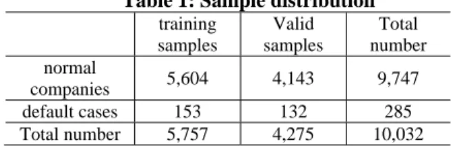
In this study, sample selection criterion is that the company has to be publicly listed as of December 2010. Accordingly, credit clients' data between January 2001 and December 2010 have been collected from banks in Taiwan as samples. The financial information used in this study are mainly combined statements, supplemented by individual statements. 10,032 observations have been collected, excluding data with omission,which include 285 default cases and 9747 normal companies. In order to apply to the model, we classify the samples into training samples and valid samples. The sample distribution is summarized in table 1.
Table 1: Sample distribution
training samples
Valid samples
Total number normal
companies 5,604 4,143 9,747 default cases 153 132 285 Total number 5,757 4,275 10,032
B. Selection of Variables
(a).Selecting Common Variables
There are more than a hundred variables generated from a company's financial statement analysis; however, it is doubtful if each variable can be used to explain the default occurrence of the company. Therefore, we will first make reference to the variables selection of famous research institutions in Taiwan and around the world, as well as those adopted by representative papers.
The industry characteristics and sampling quantities adopted by the Taiwan Corporate Credit Risk Index (TCRI), which evaluates public companies
(non-financial), conform to the research requirements of this paper. Therefore, we have made reference to the variables used in the TCRI rating. According to the TCRI, a good company should be profitable, with asset management efficiency, sound financial planning and a market leader. Accordingly, we use the following four dimensions of financial indicators: profitability, efficiency, security and size.
The Falkenstein (2000) model uses variables from six dimensions (profitability, security, size, liquidity, efficiency and growth ability) and compares the correlation between financial ratios and default probability under each dimension to choose the most suitable variables to be used in the model. Finally, 10 financial ratios are chosen to build the statistical model.
In 1968, Edward I Altman used a number of variables to conduct estimation for company failures. There were 22 financial ratios used for validation, including liquidity, profitability, financial leverage, repayment capability and efficiency. Eventually, the five ratios with best predictive power were selected for the statistical modeling.
According to the empirical experience of TCRI in credit rating, the credit risks of a company are not completely reflected in the financial ratios and many risks are actually reflected in non-financial data. Therefore, in this paper we will also consider the following variables: opinions of accountants, related-parties purchase-sales ratio, directors' pledge ratio, P/E ratio, P/B ratio and compound Return on Equity.
Due to various reasons, a company may adopt financial ratios to make its books look better. If this is the case, we may not find out the real situation about the company by judging the financial ratios only. For example, a company may borrow in the name of its subsidiary by endorsing the loan. In light of the consideration that financial ratios may not reflect the real stories, in this research, we also calculate the "adjusted" financial ratios, including: recurring net profit, debt-to-equity ratio, long-term profitability indicators.
(b). Selecting best variables for each model
Even after the above variables screening, we still come up with a large number of variables. Each of these variables may not necessarily has explanatory power about our sample companies; besides, if there are too many variables included in the model, the model will become too complicated, and collinearity problem among variables may arise, leading to unreasonable estimation of parameters. In addition, the variables that can explain default probabilities may vary among different models. Therefore, in the following, we will evaluate the variables suitable for each model so that models with the best statistical explanatory power can be built.
Regarding Logit Model, Probit Model and Survival Analysis, in the process of variables selection, first we put the independent variables into two groups, depending on whether the company is defaulting or not; then we use the SPSS (software for quantitative data analysis) to carry out two-tailed T-tests for independent samples. At the confidence coefficient of 0.05, mean differences are tested and variables with significant differences
(P-Value<0.05) will be chosen; then single-variable regression will be carried out to each independent variable, with the purpose to select those variables with higher explanatory power (P-Value<0.05); if there are concerns that the existence of high correlation among the variances will lead to collinearity, Pearson correlation analysis will be carried out to the variables selected so as to exclude those variables with high correlation. Through these steps, qualified variables under each dimension will be chosen to be input into the model.
As for Discriminant Analysis, we will first carry out single-variable discriminant analysis for each independent variable and select those variables with higher explanatory power (P-Value<0.05). If there are concerns that the existence of high correlation among the variances will lead to collinearity, the abovementioned correlation analysis will be adopted to exclude those variables with high correlation. Finally, one to two variables will be chosen under each dimension for the model.
For Artificial Neural Network analysis, there are no hypothesis limitations or collinearity problems among variables. In order to compare the model's efficiency
with the models, in the process of building the Artificial Neural Network model, we have summarized the variables used in other models for listed and non-listed companies. However, the following should be paid attention to when using the Artificial Neural Network: firstly, the number of hidden-layer neurons - the network is sensitive to the number of hidden-layer neurons, low number of neurons will fail to fit, while excessive neurons will lead to over-fitting; secondly, the number of training and learning rates - the two variables will affect the stability and convergence of the model. In consideration of these factors, when using the Artificial Neural Network, we have assumed the following parameters:
(1) Number of training: 10,000 and 20,000 times (2) Learning target: MSE<10-5
(3) Learning rate: 0.01 and 0.05
(4) Number of hidden-layer neurons: 2, 4, 6, 8, 10 Based on the above settings, regarding the combination of different parameters, we have identified the best sets of parameters under each set of data through trial and error.
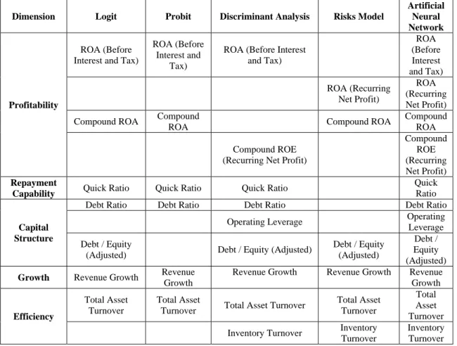
The results of best variables set selected in the above methods for each model are summarized in Table 2.
Table 2: Variables used in Different Models
Dimension Logit Probit Discriminant Analysis Risks Model
Artificial Neural Network
Profitability
ROA (Before Interest and Tax)
ROA (Before Interest and
Tax)
ROA (Before Interest and Tax)
ROA (Before Interest and Tax) ROA (Recurring
Net Profit)
ROA (Recurring Net Profit) Compound ROA Compound
ROA Compound ROA Compound
ROA Compound ROE
(Recurring Net Profit)
Compound ROE (Recurring Net Profit) Repayment
Capability Quick Ratio Quick Ratio Quick Ratio
Quick Ratio
Capital Structure
Debt Ratio Debt Ratio Debt Ratio Debt Ratio Operating Leverage Operating Leverage Debt / Equity
(Adjusted) Debt / Equity (Adjusted)
Debt / Equity (Adjusted)
Debt / Equity (Adjusted) Growth Revenue Growth Revenue
Growth
Revenue Growth Revenue Growth Revenue Growth
Efficiency
Total Asset Turnover
Total Asset
Turnover Total Asset Turnover
Total Asset Turnover
Total Asset Turnover Inventory Turnover Inventory
Turnover
Inventory Turnover
(c). Selection of Common variables
The basis of the above models comparison is that for each model, the best variables set has been selected. However, under such basis, the sets of variables vary among the models. Here we want to establish a combination of common variables that is applicable to
each model. In order to do so, we are going to select several representative variables, so as to evaluate the efficiency of each model with the common variables set. With reference to the usage of variables in the models, several representative variables have been selected from respective dimensions, which are:
Table 3: Table of Common Variables
Dimension Selected Variance
Profitability
ROA (Before Interest and Tax) Compound ROA Repayment Capability Quick Ratio
Activity Total Asset Turnover
Growth Revenue Growth Financial Structure Debt / Equity
A good independent variable shall have significant explanatory power on the dependent variables. We want to conduct a statistical analysis to validate if the selected variables have good explanatory power over the default probability. The most common method used for such purpose is regression; therefore, we will use regression to
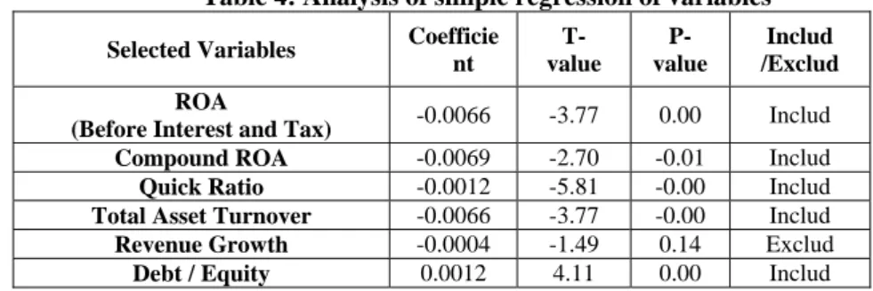
validate the variables. As to the estimation of default probabilities, we have made reference to the research by Xue Ren-rui, Liu Ying-feng.After we have obtained the default probabilities, we have conducted simple regression analysis to the variables using the weighted least squares method, so as to find out if each variable has significant explanatory power to the default probabilities. Table 4 is the analysis results. From Table 4, we can see that other than revenue growth, all variables can significantly explain the default probabilities. Through the above selection of variables, from the variables that we have selected arbitrarily, we can find out those that are proven by statistical inference to be closely related to default probabilities.
Table 4: Analysis of simple regression of variables
Selected Variables Coefficie nt
T- value
P- value
Includ /Exclud ROA
(Before Interest and Tax) -0.0066 -3.77 0.00 Includ
Compound ROA -0.0069 -2.70 -0.01 Includ
Quick Ratio -0.0012 -5.81 -0.00 Includ
Total Asset Turnover -0.0066 -3.77 -0.00 Includ Revenue Growth -0.0004 -1.49 0.14 Exclud
Debt / Equity 0.0012 4.11 0.00 Includ
As "Industry" is a dummy variable, regression cannot be used to verify its correlation with the default probabilities. In this research we assume it is a significant variable without testing.
In order to test if collinearity exists among the selected variables, we also look at the VIF values. The VIF values of the variables are calculated and listed in Table 5.
Table 5: Table of VIF of Selected Variables
Selected Variables VIF Value Included/Excluded ROA
(Before Interest and Tax)
2.3122 Included
Compound ROA 2.1243 Included
Quick Ratio 1.3848 Included
Total Asset Turnover 1.2623 Included
Debt / Equity 1.3717 Included
From Table 5, only Return on Assets Ratio (Before Interest and Tax) and Compound Return on Assets Ratio generate higher VIF values. Based on the usual standard that VIF less than 10 will not jeopardize the parameter estimates, we infer that there are no multi-collinearity issues with the above variables.
(d). Validation
We have conducted regression to the best variables and common variables of each model ,we can define the accuracy ratio of each model as the numbers of companies whose regression results are in conformity with physical facts divided the numbers of observations (10,032) .In order to verify the efficiency of the variables in the models, we have listed out the accuracy ratios of the models with the best variables set and common variables set respectively in Table 6 and Table 7:
Table 6: Accuracy Ratio of Each Model with the Best Variables Set
Model Accuracy Ratio
Merton Option Pricing
Logit Regression
Probit Regression
Discriminant Analysis
Hazard Ratio
Artificial Neural Network
In-Sample N/A* 0.9566 0.9556 1.0000 0.8044 1.0000
Out-Sample 0.4667 0.9111 0.9289 0.9378 0.7778 0.8756
Note: As the Merton model does not require In-Sample parameters, such data is not available
Table 7: Accuracy Ratio of Each Model with the Common Variables Set
Model Accuracy Ratio
Merton Option Pricing
Logit Regression
Probit Regression
Discriminant
Analysis Hazard Ratio
Artificial Neural Network
In-Sample N/A* 0.9578 0.9378 0.9589 0.7956 1.0000
From the validation results, we can see that the accuracy ratios of using common variables set are similar to the accuracy ratios using best variables set. This demonstrates it is feasible to establish a common variables set which can be applied to different models. C.Credit default probabilities
During validation, we have obtained the default probabilities of each sample company under different models. Once we have a representative probability rate
(score) for each sample, we can carried out the grading with the scores.
Regarding the estimation of default probabilities, the most direct approach is to acquire the ratings of the samples in different periods, and obtain the long run average estimated default probabilities under each grade by building a transition matrix.
Take Logit Model as an example; based on the rating results in 2005 & 2006 and information of default occurrence of the companies in 2006, we can build a transition matrix as in Table 8.
Table 8: 2005-2006Transition Matrixes
1 2 3 4 5 6 7 8 9 10 Default
1 72% 16% 8% 0% 0% 3% 0% 1% 0% 0% 0% 2 9% 53% 26% 3% 5% 2% 2% 2% 0% 0% 0% 3 12% 10% 39% 25% 14% 2% 0% 3% 3% 2% 0% 4 0% 4% 19% 33% 23% 17% 4% 0% 0% 0% 0% 5 0% 0% 5% 15% 41% 26% 8% 5% 0% 0% 0% 6 0% 2% 2% 3% 14% 34% 29% 14% 2% 0% 2% 7 0% 0% 0% 0% 3% 24% 31% 29% 3% 0% 9% 8 0% 0% 0% 2% 0% 7% 11% 40% 28% 7% 4% 9 0% 0% 0% 0% 0% 1% 1% 22% 46% 26% 5% 10 0% 0% 0% 0% 0% 2% 0% 0% 12% 65% 22% The data in transition matrix represents the probability
that credit quality migrate from some rate to another rate after a year. This probability can be calculated as follows:
1 , ,
0 ,
j i j
j
n P
n =
0,j
n
is the number of companies with credit rating i at t=0,
n
1,j is the number of companies with credit rating j at t=1.If data deficiencies result in banks failing to estimate default probabilities, we need quantify the internal ratings by use of other approaches. By Carey、Hrycay (2001), Mapping method can be used to calculatedefault probabilities.
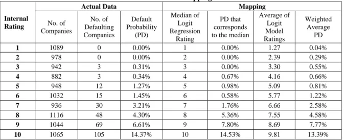
Based on the above mentioned internal rating results, using the rating results of Logit Model as indicators, we find out the default probabilities from internal ratings by various mapping methods including judgmental, mechanical and weighted average mappings.
Table 9: Simulation Mapping Results
Internal Rating
Actual Data Mapping
No. of Companies
No. of Defaulting Companies
Default Probability
(PD)
Median of Logit Regression
Rating
PD that corresponds to the median
Average of Logit Model Ratings
Weighted Average
PD
1 1089 0 0.00% 1 0.00% 1.27 0.04% 2 978 0 0.00% 2 0.00% 2.39 0.29% 3 942 3 0.31% 3 0.00% 3.30 0.55% 4 882 3 0.34% 4 0.67% 4.16 0.66% 5 948 12 1.27% 5 0.98% 5.09 0.81% 6 1032 15 1.45% 6 0.58% 5.77 1.22% 7 936 30 3.21% 7 1.76% 6.66 2.58% 8 1116 48 4.30% 8 5.36% 7.55 4.58% 9 1044 69 6.61% 9 7.80% 8.69 7.77% 10 1065 105 14.37% 10 14.53% 9.81 13.39% Under Judgmental mapping, at first we map internal
grades to external grades subjectively, then take default probabilities from external ratings as probabilities from internal ratings. Under mechanical mapping, we sort the company in each internal grade by corresponding external grades, and then take the median of average default probabilities in external grades as default probabilities in
each internal grade. Under weighted average mapping, we take the weighted average of average default probabilities in external grades corresponded to internal grades as default probabilities in each internal grade. Due to Judgmental mapping is lack of logical basis, we just calculate the default probabilities with mechanical
mapping and weighted average mapping respectively (see Table9).
We can see that it is more suitable to use median to compute the actual default probability for the safe grades
(1~4), while it is better to use weighted average to estimate actual default probability for the risky grades (8~10).
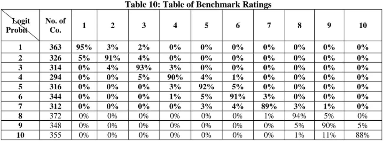
Table 10: Table of Benchmark Ratings
Logit Probit
No. of
Co. 1 2 3 4 5 6 7 8 9 10
1 363 95% 3% 2% 0% 0% 0% 0% 0% 0% 0%
2 326 5% 91% 4% 0% 0% 0% 0% 0% 0% 0%
3 314 0% 4% 93% 3% 0% 0% 0% 0% 0% 0%
4 294 0% 0% 5% 90% 4% 1% 0% 0% 0% 0%
5 316 0% 0% 0% 3% 92% 5% 0% 0% 0% 0%
6 344 0% 0% 0% 1% 5% 91% 3% 0% 0% 0%
7 312 0% 0% 0% 0% 3% 4% 89% 3% 1% 0%
8 372 0% 0% 0% 0% 0% 0% 1% 94% 5% 0% 9 348 0% 0% 0% 0% 0% 0% 0% 5% 90% 5% 10 355 0% 0% 0% 0% 0% 0% 0% 1% 11% 88% To validate the default probabilities, we adopt
benchmark comparisons for empirical explanations. Continue with the above analysis using the results corresponding to the medians under mapping, we use Logit Model as benchmarks for ratings comparison. Then carry out the benchmarks comparison to the Probit Model. The data represents the distribution of the number of some rate under logit model. For example, when the rate is 1 under logit model, 95%number of company belongs to 1 under probit model; only 5% number of company is other rate. The results are shown in Table 10.
From Table 10, we can see that the comparison results for each grade are acceptable. Consequently, we can build a credit scoring model based on these findings.
V. CONCLUSION
The effectiveness of credit risks management relies on whether it can operate with the local environment. Therefore, choosing the variable set that fits in with the local conditions is critical to the performance of a credit rating model. But most of researchers always choose corresponding variables for different model. In this paper, we have adopted Merton Option Pricing Model, Discriminant Analysis Model, Regression Analysis Models (Logit Model and Probit Model), Survival Analysis Model and Artificial Neural Network Model in finding the common variables set for application in credit risks management models.Our findings show that five variables, namely Return on Assets Ratio (Before Interest and Tax), Compound Return on Assets Ratio, Quick Ratio,Total Asset Turnover, Debt-to-EquityRatio, are applicable to different credit risk rating models.Moreover, this paper estimates long term average default probability by using Transition Matrix and Mapping method. Validation findings also show that they have good forecasting abilities. Such findings help to simplify the application of credit risks management models and better adapt the models to the local conditions in China. We believe that the research methods presented in this paper can also be applied to other countries or regions around the worlds. It can serve as a good
reference for establishing credit risks management models that fit with the local conditions.
ACKNOWLEDGMENT
This work was supported by the Fundamental Research Funds for the Central Universities (2010221040), China National Social Science Fund (09AZD045), Ministry of Education for Humanities and Social Sciences (08JA630004), Anhui Provincial Natural Science Research Project for Universities (KJ2010A072) and China National Bureau of Statistics Fund (2009LZ045). We would like to thank the editor, associate editor, and referees for careful review and insightful comments, which have led to significant improvement of the article.
REFERENCES
[1] Basel Committee on Banking Supervision (1999), Credit Risk Modeling: Current Practice and Application, Bank for International Settlements.
[2] Basel Committee on Banking Supervision (2003), Consultative Document: The New Basel Capital Accord, Bank for International Settlements.
[3] Carey, Mark and M. Hrycay (2001), Parameterzing credit risk models with rating data, Journal of Banking & Finance 25, p. 197-270
[4] Division of Banking Supervision and Regulation (1998), Bank Holding Company Supervision Manual, Board of Governors of the Federal Reserve System
[5] Division of Banking Supervision and Regulation(2003), Draft Supervisory Guidance on Internal Ratings-Based Systems for Corporate Credit, Board of Governors of the Federal Reserve System
[6] Engelmann, Bernd, E. Hayden and D. Tasche (2003), Testing Rating Accuracy, Risk Falkenstein, E., A. Boral, and L. Carty (2000), RiskCalc Private Model: Moodys Default Model for Private Firms, Moodys Investors Service.
[7] Ferguson Jr., Roger W. (2003), Basel II: Some Issues for Implementation,Basel Sessions 2003 Speech, Institute of International Finance, New York .
[8] Keenan, S. C. and J. R. Sobehart (2001), Performance Measures for Credit Risk Models, Moody’s Risk Management Services Research Report.