Machine learning approach for flood risks prediction

ISSN: 2252-8938, DOI: 10.11591/ijai.v9.i1.pp73-80  73

Machine learning approach for flood risks prediction

1,3_{Faculty of Computer Science and Information Technology, Universiti Tun Hussein Onn Malaysia, 86400 Batu}

Pahat, Johor, Malaysia.

2_{Faculty of Applied Sciences and Technology, Universiti Tun Hussein Onn Malaysia, 86400 Batu Pahat, Johor, Malaysia}

Article Info ABSTRACT

Article history: Received Aug 20, 2019 Revised Nov 28, 2019 Accepted Dec 16, 2019

Flood is one of main natural disaster that happens all around the globe caused law of nature. It has caused vast destruction of huge amount of properties, livestock and even loss of life. Therefore, the needs to develop an accurate and efficient flood risk prediction as an early warning system is highly essential. This study aims to develop a predictive modelling follow Cross-Industry Standard Process for Data Mining (CRISP-DM) methodology by using Bayesian network (BN) and other Machine Learning (ML) techniques such as Decision Tree (DT), k-Nearest Neighbours (kNN) and Support Vector Machine (SVM) for flood risks prediction in Kuala Krai, Kelantan, Malaysia. The data is sourced from 5-year period between 2012 until 2016 consisting 1,827 observations. The performance of each models were compared in terms of accuracy, precision, recall and f-measure. The results showed that DT with SMOTE method performed the best compared to others by achieving 99.92% accuracy. Also, SMOTE method is found highly effective in dealing with imbalance dataset. Thus, it is hoped that the finding of this research may assist the non-government or government organization to take preventive action on flood phenomenon that commonly occurs in Malaysia due to the wet climate.

Keywords: Bayesian Network Decision Tree Flood Prediction k-Nearest Neighbour Support Vector Machine

This is an open access article under the CC BY-SA license.

Corresponding Author: Shuhaida Ismail,

Faculty of Applied Sciences and Technology, Universiti Tun Hussein Onn Malaysia, 86400 Batu Pahat, Johor, Malaysia. Email: [email protected]

1. INTRODUCTION

Flood is the most common natural disaster that happened all around the world. Countries that experience flood event need to face a huge of amount property destruction, environmental and financial losses even fatalities among the citizen. There are several impactful factors that affect the inconsistency flood occurrence such as temperature, humidity, dew point temperature, wind speed, streamflow volume, water level and rainfall volume. The streamflow volume indicates the river capability in holding the water in order to sustain the rainfall volume. Higher temperature and wind speed resulted in faster water particles moves, thus easier to evaporate into the atmosphere. Humidity also affects the water particle in the air to be condensed out of the atmosphere. Previous studies on flood detection has been done due to disastrous event occur in countries such as in disastrous flood event occur in Australia [1], Malaysia [2], India [3] and many other countries. Malaysia located geographically near the equatorial line which prevent it from severe natural disaster phenomenon such as earthquakes, volcanic eruption and typhoons. However, Malaysia experience hot and humid weather by average daily temperature of 21°C to 32°C throughout the year since Malaysia influenced heavily by equatorial line.

In addition, Malaysia also experience climate changes of north eastern monsoon from November to March and the western monsoon from June to October. Due to monsoon season, the annual rainfall in Malaysia quite high by 2500 mm in Peninsular Malaysia, 2300 mm in Sarawak and 3300 mm in Sabah. However, monsoon in Peninsular Malaysia contributes 86% from the annual rainfall in east coast of Malaysia consisting the states of Kelantan, Terengganu and Pahang. The heavy rainfall usually resulted in flood whether natural or flash flood. For instance, the disastrous flood event occurred in 2014 [4] has given important lesson of having flood prediction system to monitor, predict, and detect the flood event. In order to reduce such damages, an early issued flood warning is essential. Thus, water level forecasting is essential to predict future flood occurrence. Water level prediction also benefits other sectors such as agriculture, plants, domestics and industrial and commercial [5]. The aim of this research paper is to develop a predictive modelling which follow Cross-Industry Standard Process for Data Mining (CRISP-DM) methodology by using Bayesian network (BN) and other Machine Learning (ML) techniques such as Decision Tree (DT), k-Nearest Neighbours (kNN) and Support Vector Machine (SVM) for flood risks prediction in Kuala Krai, Kelantan, Malaysia. The remaining of this paper is organized as follows. Section 2 reviews all works related to techniques used for flood risk prediction. Section 3 presents the data mining methodology as well as dataset pre-processing, experimental setup, and the evaluation metrics. Section 4 presents the results and finally Section 5 concludes with some directions for future work.

2. RELATED WORK

Application of BN and other ML techniques in prediction and classification has been used widely in many field including agriculture, economy, and etc in Malaysia. [6] Used ML techniques such as an Artificial Neural Network (ANN), K-Nearest Neighbours (kNN), Decision Table (DT) and M5P Tree algorithms in their research to classify herbs for agriculture industry in Malaysia since this industry is crucial to assist the economy development of Malaysia as one of leading exporter of herbs. Meanwhile, [7] has proposed new Halal technologies using ML technique to facilitate the Muslim consumers in Malaysia to authenticate the Halal logo image not just locally but also globally as long it were recognised by the Malaysian’s Department of Islamic Development (JAKIM). However, recent work of application of BN and ML techniques have been used widely focusing on natural disaster detection such as flood risks detection.

In 2018, [2] has carried out research on predicting flood risks using Bayesian approaches. They conducted experiment using three Bayesian classifier algorithms namely general Bayesian Networks, naive Bayes and Tree Augmented Naive Bayes to predict the flood risks in Kuala Krai, Kelantan, Malaysia for 5-years. The results showed that general Bayesian Networks successfully outperformed both Naive Bayes and tree augmented naive Bayes in term of accuracy. This paper has been used as our anchor paper to conduct further research by comparing Bayesian network (BN) with other ML techniques such as Decision Tree (DT), k-Nearest Neighbours (kNN) and Support Vector Machine (SVM). [8] Proposed an early prediction system using Autoregressive Neural Networks with Exogenous Input (NNARX) for 5-hour ahead for flood. Water level and rainfall for various stations located in Kelantan, Malaysia were observed. The performance of proposed NNARX were compared with conventional Neural Network for prediction performance. The results showed that NNARX has smallest value of Root Mean Square Error (RMSE) compared to conventional Neural Networks. Besides, [9] also focusing on flood event in Kelantan, Malaysia. They proposed Spiking Neural Network to predict the flood risk event. Meanwhile, [10] has introduced a semi-supervised ML model, which is Weakly Labelled SVM (WELLSVM)to predict urban flood based on data samples collected from urban areas in Beijing for 10-year between 2004 to 2014. The samples consisted of nine dominant factors of metrological, geographical and anthropogenic. The model were then evaluated and compared with other two model built from Logistic Regression and Artificial Neural Networks in terms of accuracy, precision, recall and f-score. The results showed that WELLSVM flood successfully outperformed both models because WELLSVM has the advantage in utilizing the unlabelled data.

In some other cases, [11] proposed a model based on ensemble classifier for more precise water flooded layer recognition which means the target classes are divided into four target classes, which are the oil layer, weak water flooded, middle water flooded and strong water flooded. Interestingly, this model was used to predict the water flooded layer in oil or gas reservoir. The ensemble classifier were made up of the model-free classification (MFBC) algorithm, the k-Nearest Neighbours (kNN) algorithm and the Support Vector Machine (SVM) algorithm which were then validated and evaluated. The dataset went through oversampling process using Synthetic Minority Over sampling Technique (SMOTE) due to imbalance classes. The results showed that the ensemble classifier performed better as compared to MFBC, KNN and SVM for both UCI data and chromatogram data while all three MFBC, KNN and SVM were similar in accuracy for 90% and 70.59% respectively. Finally, the destructive flood event at Australia in 2011 has urged [1] to use two ML approaches; DT and SVM to evaluate spatial correlations between the contributing factors to flood and rate

the factors according to their importance in mapping the flood prone areas. The results showed that DT was slightly better in accuracy as compared to SVM whereby DT achieved 89% and SVM achieved 87% in the first dataset and low in accuracy as compared to SVM in the second dataset by DT (89%) and SVM (87%) respectively.

3. RESEARCH METHOD

This project adopted the Cross-Industry Standard Process for Data Mining (CRISP-DM) [12]. This methodology divided data mining task into six phases as shown in Figure 1. The six phases comprises of business understanding, data understanding, data preparation, modelling, evaluation and deployment. This CRISP-DM has become a benchmark or standard methodology to be follow in data mining task project completion. Each of the phases in CRISP-DM will produce output that benefits the flow of data mining project as whole. It make the project more flexible and efficient to solve business issues using analytics. Table 1 described in brief the six major steps in CRISP-DM.

Figure 1. CRISP-DM methodology [12].

Table 1. CRISP-DM methodology CRISP-DM

steps

Description 1. Business

Understanding

Focuses on understanding the research objectives and requirements, and then converting this knowledge into a data mining problem definition. 2. Data

Understanding

Focuses on data collection, and proceed with investigating and studying the data to identify data quality problems, to discover first insights into the data, or to detect interesting subsets to form hypotheses for hidden information. 3. Data

Preparation

The data preparation phase or also known as data preprocessing covers all activities to construct the final dataset from the initial raw data and to ensure the data be used is improved in quality and acceptable before modelling phase. Include cleansing, transformation, discretization, reduction and feature engineering.

4. Modeling Modelling techniques such as machine learning algorithms are selected and applied. Can be loop back to data preparation phase accordingly to suitability of datasets with applied algorithms 5. Evaluation Focuses on evaluate and validate the models that

have been built for measuring the quality and performance of the models considering the objectives and requirements. The model which successfully obtained the highest quality and performance will be selected as end product. 6. Deployment This last phase is to deploy the end product to be

applied in real world situation.

3.1. Dataset

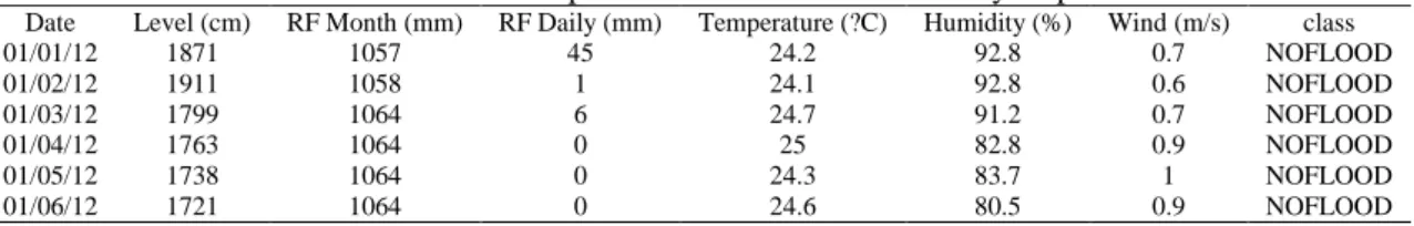
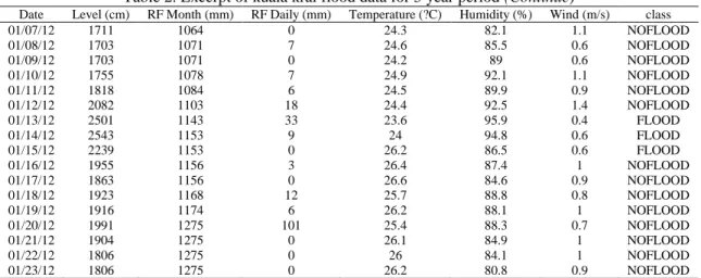
All the dataset were extracted from [13-14] which are 5 year period records of flood data in Kuala Krai, Kelantan, Malaysia between 1st January 2012 until 31st December 2016 consisting of 1,827 instances and 8 features including date, rainfall monthly, rainfall daily, water level, humidity, wind and the binary target class whether flood or not which are correspond features for flood risks prediction. Note that ’date’ feature were not included in the experimental process since it contain unique value for each instances which not gave any significant impact to learning process. The part of sample data accordingly to the features are shown in Table 2.

Table 2. Excerpt of kuala krai flood data for 5 year period

Date Level (cm) RF Month (mm) RF Daily (mm) Temperature (?C) Humidity (%) Wind (m/s) class 01/01/12 1871 1057 45 24.2 92.8 0.7 NOFLOOD 01/02/12 1911 1058 1 24.1 92.8 0.6 NOFLOOD 01/03/12 1799 1064 6 24.7 91.2 0.7 NOFLOOD 01/04/12 1763 1064 0 25 82.8 0.9 NOFLOOD 01/05/12 1738 1064 0 24.3 83.7 1 NOFLOOD 01/06/12 1721 1064 0 24.6 80.5 0.9 NOFLOOD

Table 2. Excerpt of kuala krai flood data for 5 year period (Continue)

Date Level (cm) RF Month (mm) RF Daily (mm) Temperature (?C) Humidity (%) Wind (m/s) class 01/07/12 1711 1064 0 24.3 82.1 1.1 NOFLOOD 01/08/12 1703 1071 7 24.6 85.5 0.6 NOFLOOD 01/09/12 1703 1071 0 24.2 89 0.6 NOFLOOD 01/10/12 1755 1078 7 24.9 92.1 1.1 NOFLOOD 01/11/12 1818 1084 6 24.5 89.9 0.9 NOFLOOD 01/12/12 2082 1103 18 24.4 92.5 1.4 NOFLOOD 01/13/12 2501 1143 33 23.6 95.9 0.4 FLOOD 01/14/12 2543 1153 9 24 94.8 0.6 FLOOD 01/15/12 2239 1153 0 26.2 86.5 0.6 FLOOD 01/16/12 1955 1156 3 26.4 87.4 1 NOFLOOD 01/17/12 1863 1156 0 26.6 84.6 0.9 NOFLOOD 01/18/12 1923 1168 12 25.7 88.8 0.8 NOFLOOD 01/19/12 1916 1174 6 26.2 88.1 1 NOFLOOD 01/20/12 1991 1275 101 25.4 88.3 0.7 NOFLOOD 01/21/12 1904 1275 0 26.1 84.9 1 NOFLOOD 01/22/12 1806 1275 0 26 84.1 1 NOFLOOD 01/23/12 1806 1275 0 26.2 80.8 0.9 NOFLOOD

3.2. Experimental setup

All the Bayesian Networks and machine learning (ML) algorithms used in this research such as Decision Trees (DT), k-Nearest Neighbours (kNN) and Support Vector Machine (SVM) algorithms fully available in the Waikato Environment for Knowledge Analysis (WEKA) [15]. The Weka software runs on Intel(R) Core (TM) i5-4200M CPU in Window 8 (64-bit) operating system with 8 GB of random access memory (RAM). The 10-fold cross validation was applied for validating the performance for each algorithm in term of accuracy, precision, recall and f-measure. Five year period of sample flood data are selected to observe the stability of performance for each Bayesian Networks and three other classifiers.

3.3. Pre-processing

The pre-processing performed in the data preparation phase is imperative before building the flood risks prediction model using the four classification algorithms, which are BN, kNN, DT and SVM. The data first required undergoing resampling process since the dataset is imbalance. Imbalance data is a classification problem that occur when the target classes are not equally distributed. For example, the dataset for flood in Kuala Krai containing about 1,795 instances of ‘no flood’ class as compared to remaining 32 instances of ‘flood’ class. According to review conducted by [16], many real world domains has imbalance data problem and it is crucial to combat imbalance data because it will negatively affect the machine learning process and driven error in classification or prediction. Resampling is one of the method to combat imbalance data. Resampling process consists of oversampling and under-sampling. Oversampling is a process to add copies or synthetic instances to under-represented class while under-sampling is a process to delete the instances from over represented class. In other word, the oversampling method called Synthetic Minority Oversampling Technique (SMOTE) has been applied to under-represented data class which are flood class by adding synthetic instances to make the data class balance. [17] Proposed the SMOTE technique to combat imbalance data by creating extra training data called synthetic data. The synthetic data were created by taking the difference between two point or neighbours from real sample data. As a result, there new dataset will be created randomly along the line segment between two specific features of real data. Thus, 1,795 instances of ’no flood’ class and 2,048 instances of ’flood’ class are produced after applying SMOTE to under-represented ’flood’ class.

3.4. Modelling

This paper is set to investigate the performance of Bayesian Networks and other machine learning techniques which are DT, kNN and SVM in predicting flood risks based on a CRISP-DM methodology. The Bayesian approach is among of well-known techniques to be used by researchers for constructing prediction model as well as three other ML techniques. Four classifiers techniques which are Bayesian Networks (BN), DT, kNN and SVM are well supported by data mining tools, WEKA for executing of experiment [18].

 Bayesian Networks (BN) or also known as Bayesian Nets or Bayesian Belief Networks (BBN) is a network structure made up of Directed Acyclic Graphs (DAG) that link features based on their conditional probabilities which then are calculated using Bayes’ Theorem [19]. [19] Also stated that BN also very useful in determine, represent and visualize the relationship among features from empirical data, expert knowledge or both empirical and expert knowledge besides determine the key of uncertainties. A K2 searching algorithm with Bayesian Dirichlet BDeu scoring metric adopted from

[20] have been used to construct BN model. Note that, the initial structure learning were set to random since the default setting in WEKA will construct naive Bayes as initial structure learning. In addition, the number of parent node is limit to five in order to avoid complexity and high computational costs.

 Decision Tree (DT) or also known as Classification and Regression Trees (CART) is one of popular ML techniques. The target class in classification trees is categorical type class while numerical type class for regression trees [21]. It is shows that trees are capable to process both discrete and continuous data. WEKA offered decision tree in its software however in this research, more advance tree algorithm, C4.5 algorithm or also known as J48 in WEKA have been used to construct the decision tree compare to basic REPTree. The setting of no pruning is set to false to allow the pruning process occur. Thus, it may reduce the complexity of tree and computational costs besides deduce data over-fitting which may increase the predictive accuracy.

 k-nearest neighbours (kNN) also supports both classification and regression same like DT. kNN is a simple algorithm that store all training dataset and call back the data to predict the k most similar with training pattern from stored dataset. So, kNN only used little computational costs in order to compute the distance between two instances for k value. In WEKA, kNN algorithm were put under the ‘lazy’ group. The default setting were Linear NN Search which used Euclidean distance as distance function parameter to calculate the distance between instances. Note that, the cross validate parameter were set to true in order to allow WEKA discover a good value for k. However, the value of k were set to 1, 3, 5 and 7 to control the size of the neighbourhood for kNN in the experiment. The best result produced by selected k value will be used as comparison with BN and other ML techniques. Note that 3 as k value produced most optimum result.

 Support Vector Machine (SVM) was actually developed for solving the binary classification problems. However, the researchers have extended the SVM to make it suitable to support multi-class classification and regression problems. SVM has the capability to handle both continuous and discrete data as it automatically normalizes the data before they are modelled. SVM then calculates a line that best isolate the data into two groups and only consider those instances that are closest to the separating line. The instances are called support vectors, hence the name of the technique. In WEKA, the SVM algorithm is implemented as the Sequential Minimal Optimization (SMO), which are the optimization algorithm used inside the SVM implementation.

3.5. Evaluation metrics

Every prediction model has its own way of validating and evaluating its performance. Evaluation is performed to compare whether there are similarity or consistency between the observed results and the predicted results or across a number of different models’ predicted results. For this research, accuracy, precision, recall and f-score has been used as evaluation metric because it has been used widely by a majority of researchers including [2, 22] for flood risks prediction compare to other evaluation metrics such as Root Mean Square Error [23] and model construction times [24]. Accuracy can be derived from a confusion matrix as shown in Table 3.

Table 3. Confusion matrix

NO (Prediction) YES(Prediction) NO (Actual) True Negative (TN) False Positive (FP) YES (Actual) False Negative (FN) True Positive (TP)

The columns represent the prediction class and rows show the actual class target. The flood outcome is represented with the label YES, and no-flood is represented with the label NO. Therefore, diagonal elements (TN, TP) in Table 2 shows the true predictions and the other elements (FN, FP) reflect the false predictions. For example, there are two outcome in the flood prediction, which are flood and no-flood. The True Positive (TP) means correct flood result prediction and True Negative (TN) means correct no-flood result prediction while False Positive (FP) means incorrect flood result prediction and False Negative (FN) means incorrect no-flood result prediction. If a target class is predicted as flood (YES) even though it is a no-flood (NO) target class, this test result is added to the FP in the table. Therefore, number FP is incremented by 1. Thus, accuracy in the confusion matrix is defined as in (1).

Accuracy = TP TN

FP TP TN FN



Precision (positive predictive value) can be defined as in (2) where the total number of correctly classified positive samples are divided by the total number of actual positive samples.

Precision = TP

FP TP

(2)

Recall (sensitivity) know can be defined as in (3) where the total number of correctly classified positive samples divided by the total number of predicted positive samples.

Recall = TP

TPFN

(3)

F-measure (F1 score or F score) can be defined as the weighted harmonic mean of the precision and recall of the samples.

2 Precision Recall F-Measure =

Precision+Recall

  ₍₄₎

4. RESULTS AND DISCUSSION

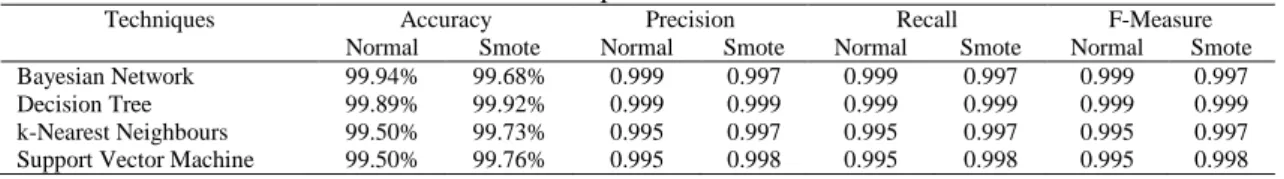
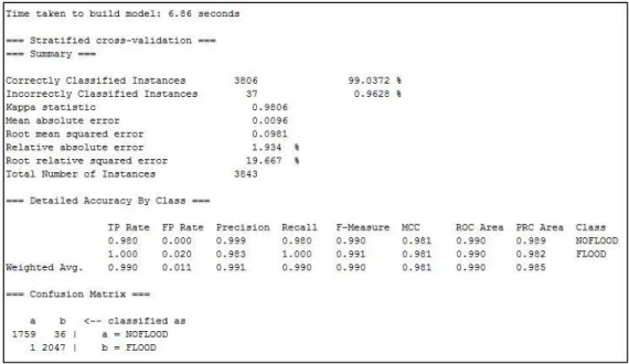
Following the previous evaluation metric used in research work carried out by [2, 22], the experimental results for BN and three other ML techniques, DT, kNN and SVM are compared in terms of accuracy, precision, recall and f-measure performance as the evaluation metric. Table 4 shows the experimental results across 5 years period of flood data from Kuala Krai, Kelantan using 10-fold cross validation. The data were divided into two, normal data and SMOTE data. Technically, the normal data actually imbalance because the target class which are flood and no flood are not equally distributed. It may cause the prediction results produce will be biased to majority target class. So, the data have been applied SMOTE method in order to combat imbalance data by adding the under-presented target class with synthetic data that derived from real data. Overall, the results shows that BN (99.94%) slightly better than other three ML techniques which are DT (99.89%), kNN (99.50%) and SVM (98.23%) however are comparable after application of SMOTE method to data by 99.68% (BN), 99.92% (DT), 99.86% (kNN) and 99.03% (SVM) as well as other metric such as precision, recall and f-measure respectively. Thus, DT achieved the highest value of precision, recall and F-measure whether in normal data and SMOTE data by 0.999. Figure 2 shows part of experimental output from WEKA using SVM based on SMOTE data. The experimental output include evaluation matrix such as accuracy, precision, recall and f-measure as well as confusion matrix of target class of ’not flood’ and ’flood’.

Table 5 shows the confusion matrix for BN and three other ML techniques, DT, kNN and SVM based on target class of ’no flood’ (NO) and ’flood’ (YES) using normal data and SMOTE data. There are some observation has been done in the experiment. For example, it is observed that the best kNN result in accuracy were produced if the value of k is set to 1 while other value of k such as 3, 5 and 7 produced slightly worse result in accuracy. In other words, when the value of k increased, the accuracy achieved by kNN will be decreased. Besides, the water level play important roles as features for flood since the feature become main rules for DT (’no flood’ if the water level lower and equal to 2182 cm and ’flood’ if the water level more than 2182 cm) and directly pointed to target class in BN. Meanwhile, BN still evolve over time and has potential to be improved further in future. [25] Claimed that BN have many advantages over other classification techniques to solve the real world problems. In their survey, they explained and discuss every discrete BN classifier that available and categorize them in three group based on factorization. They also stated that BN can be organised hierarchically from the simplest algorithm like naive Bayes to the most complex like Bayesian multiunit. However, [22] stated in their work where the continuous development of machine learning algorithms in time may expand the machine learning applications in the field of hydrology are becoming more and more extensive in the future especially on flood risk assessment.

Table 4. Experimental results

Techniques Accuracy Precision Recall F-Measure Normal Smote Normal Smote Normal Smote Normal Smote Bayesian Network 99.94% 99.68% 0.999 0.997 0.999 0.997 0.999 0.997 Decision Tree 99.89% 99.92% 0.999 0.999 0.999 0.999 0.999 0.999 k-Nearest Neighbours 99.50% 99.73% 0.995 0.997 0.995 0.997 0.995 0.997 Support Vector Machine 99.50% 99.76% 0.995 0.998 0.995 0.998 0.995 0.998

Figure 2. Excerpt of experimental output from WEKA

Table 5. Confusion matrix for all techniques based on normal data and smote data NO (Prediction) Yes (Prediction)

Bayesian Networks with normal data NO (Actual) 1795 0 YES (Actual) 1 31

Bayesian Networks with SMOTE data NO (Actual) 1793 2 YES (Actual) 10 2038

Decision Tree with normal data NO (Actual) 1793 2 YES (Actual) 0 32

Decision Tree with SMOTE data NO (Actual) 1792 3 YES (Actual) 0 2048

k-Nearest Neigbors with normal data NO (Actual) 1794 1 YES (Actual) 8 24

k-Nearest Neigbors with SMOTE data NO (Actual) 1791 4 YES (Actual) 1 2047

Support Vector Machine with normal data NO (Actual) 1795 0 YES (Actual) 9 23

Support Vector Machine with SMOTE data NO (Actual) 1786 9 YES (Actual) 0 2048

5. CONCLUSION AND FUTURE WORK

In conclusion, this research presented a flood risks prediction based on CRISP-DM methodology using BN and three machine learning (ML) techniques known as DT, kNN and SVM. The aims of this research is to develop a predictive modelling for flood risks prediction in Kuala Krai, Kelantan, Malaysia. The predictive accuracy of all models were compared and results showed that BN was slightly better using normal data. The research also found that SMOTE method are highly useful in combating with imbalance dataset. This finding is supported by the results of the models when SMOTE method are applied. Other than that, the study also found that each techniques as its own advantages and disadvantages. However, some research like [11] suggest ensembles classifier is better than BN and other ML techniques such as DT, kNN and SVM. It is also encourage to make dynamic system that can incorporate with time variation for flood prediction as the flood event is a race with time in order to plan the preventive action that must be taken in a short of time since flood is disaster that not just destroy huge amount of properties but also can cause loss of many human lives.

ACKNOWLEDGEMENTS

This research is supported by Universiti Tun Hussein Onn Malaysia via the Tier 1 Grant Scheme Vot H073

REFERENCES

[1] M. S. Tehrany, S. Jones, and F. Shabani, “Identifying the essential flood conditioning factors for flood prone area mapping using machine learning techniques,” Catena, vol. 175, no. April, pp. 174–192, 2019.

[2] N. I. M. Roslin, A. Mustapha, N. A. Samsudin, and N. Razali, “A bayesian approach to prediction of flood risks,”

International Journal of Engineering and Technology, vol. 7, no. 4.38, pp. 1142–1145, 2018.

[3] E. Venkatesan and A. B. Mahindrakar, “Forecasting floods using extreme gradient boosting – a new approach,”

International Journal of Civil Engineering and Technology, vol. 10, no. 2, pp. 1336–1346, 2019.

[4] M. Othman, A. A. Latif, S. S. Maidin, M. F. M. Saad, and M. N. Ahmad, Engagement of Local Heroes in Managing Flood Disaster: Lessons Learnt from the 2014 Flood of Kemaman, Terengganu, Malaysia. Intech Open, 2018.

[5] V. Yadav and K. Eliza, “A hybrid wavelet-support vector machine model for prediction of lake water level fluctuations using hydro-meteorological data,” Journal of the International Measurement Confederation, vol. 103, pp. 2655–2675, 2017.

[6] A. D. A. Dali, N. A. Omar, and A. Mustapha, “Data mining approach to herbs classification,” Indonesian Journal of Electrical Engineering and Computer Science, vol. 12, no. 2, pp. 570–576, 2018.

[7] S. F. A. Razak, C. P. Lee, K. M. Lim, and P. X. Tee, “Smart halal recognizer for muslim consumers,” Indonesian Journal of Electrical Engineering and Computer Science, vol. 14, no. 1, pp. 193–200, 2019

[8] M. A. S. Anuar, R. Z. A. Rahman, S. B. Mohd, A. C. Soh, and Z. D. Zulkafli, “Early prediction system using neural network in kelantan river, malaysia,” in Proceedings of the 15th IEEE Student Conference on Research and

Development: Inspiring Technology for Humanity, SCOReD 2017, 2018, pp. 104–109.

[9] M. Abdullah, M. Othman, S. Kasim, and S. Mohamed, “Evolving spiking neural networks methods for classification problem: a case study in flood events risk assessment,” Indonesian Journal of Electrical Engineering

and Computer Science, vol. 16, no. 1, pp. 222–229, 2019.

[10] G. Zhao, B. Pang, Z. Xu, D. Peng, and L. Xu, “Assessment of urban flood susceptibility using semi-supervised machine learning model,” Science of the Total Environment, vol. 659, no. 3, pp. 940–949, 2019.

[11] Z. Geng, X. Hu, Q. Zhu, Y. Han, Y. Xu, and Y. He, “Pattern recognition for water flooded layer based on

ensemble classifier,” in Proceedings of the 5th International Conference on Control, Decision and Information

Technologies, CoDIT 2018, 2018, pp. 164–169.

[12] R. Wirth and J. Hipp, “Crisp-dm: Towards a standard process model for data mining,” in Proceedings of the 4th

international conference on the practical applications of knowledge discovery and data mining. Citeseer, 2000, pp. 29–39.

[13] The officital web of public infobanjir. [Online]. Accessed on: Nov. 24, 2019. Available: http://publicinfobanjir.water.gov.my/

[14] Laman web rasmi jabatan meteorologi Malaysia. [Online]. Accessed on: Nov. 24, 2019. Available: http://www.met.gov.my/

[15] I. H. Witten, E. Frank, M. A. Hall, and C. J. Pal, Data Mining: Practical machine learning tools and techniques. Morgan Kaufmann, 2016.

[16] H. Ali, M. N. M. Salleh, R. Saedudin, K. Hussain, and M. F. Mushtaq, “Imbalance class problems in data mining: A review,” Indonesian Journal of Electrical Engineering and Computer Science, vol. 14, no. 3, pp. 1552–1563, 2019.

[17] N. V. Chawla, K. W. Bowyer, L. O. Hall, and W. P. Kegelmeyer, “Smote: Synthetic minority over-sampling technique,” Journal of Artificial Intelligence Research, vol. 16, pp. 321–357, 2002.

[18] J. Brownlee, “How to use classification machine learning algorithms in weka”, Aug. 22, 2019. Accessed on: Nov. 24, 2019. [Online]. Available: https://machinelearningmastery.com/use-classification-machine-learning-algorithms-weka/

[19] B. G. Marcot and T. D. Penman, “Advances in bayesian network modelling: Integration of modelling technologies,” Knowledge-Based Systems, vol. 22, pp. 386–393, 2019.

[20] M. G. Madden, “On the classification performance of tan and general bayesian networks,” Environmental Modelling and Software, vol. 22, no. 2, pp. 489–495, 2009.

[21] N. Yadav, A. Kumar, R. Bhatnagar, and V. K. Verma, “City crime mapping using machine learning techniques,” in

Proceedings of the 4th International Conference on Advanced Machine Learning Technologies and Applications, AMLTA 2019, vol. 921, 2020, pp. 656–668.

[22] X. Li, D. Yan, K. Wang, B. Weng, T. Qin, and S. Liu, “Flood risk assessment of global watersheds based on multiple machine learning models,” Water, vol. 11, no. 1654, pp. 1–18, 2019.

[23] Y. Wu, W. Xu, J. Fengt, S. Palaiahnakote, and T. Lu, “Local and global bayesian network based model for flood prediction,” in Proceedings of the 24th International Conference on Pattern Recognition, ICPR 2018, pp. 225–230,

2018.

[24] A. Hesar, H. Tabatabaee, and M. Jalali, “Structure learning of bayesian networks using heuristic methods,”

Pertanika Journal of Science and Technology, vol. 45, pp. 246–250, 2012.