MapSplice: Accurate mapping of RNA-seq reads for
splice junction discovery
Kai Wang
1, Darshan Singh
2, Zheng Zeng
1, Stephen J. Coleman
3, Yan Huang
1,
Gleb L. Savich
4, Xiaping He
4, Piotr Mieczkowski
4, Sara A. Grimm
4, Charles M. Perou
4,
James N. MacLeod
3, Derek Y. Chiang
4, Jan F. Prins
2and Jinze Liu
1,*
1
Department of Computer Science, University of Kentucky, Lexington, KY 40506, 2Department of Computer
Science, University of North Carolina, Chapel Hill, NC 27599-3175,3Gluck Equine Research Center,
Department of Veterinary Science, University of Kentucky, Lexington, KY 40546-0099 and4Department of
Genetics and UNC Lineberger Comprehensive Cancer Center, University of North Carolina, Chapel Hill, NC 27599-7295, USA
Received April 25, 2010; Revised June 21, 2010; Accepted June 28, 2010
ABSTRACT
The accurate mapping of reads that span splice junctions is a critical component of all analytic tech-niques that work with RNA-seq data. We introduce a second generation splice detection algorithm, MapSplice, whose focus is high sensitivity and spe-cificity in the detection of splices as well as CPU and memory efficiency. MapSplice can be applied to both short (<75 bp) and long reads (75 bp). MapSplice is not dependent on splice site features or intron length, consequently it can detect novel
canonical as well as non-canonical splices.
MapSplice leverages the quality and diversity of read alignments of a given splice to increase
accuracy. We demonstrate that MapSplice
achieves higher sensitivity and specificity than TopHat and SpliceMap on a set of simulated RNA-seq data. Experimental studies also support the accuracy of the algorithm. Splice junctions
derived from eight breast cancer RNA-seq
datasets recapitulated the extensiveness of alterna-tive splicing on a global level as well as the
differ-ences between molecular subtypes of breast
cancer. These combined results indicate that
MapSplice is a highly accurate algorithm for the alignment of RNA-seq reads to splice junctions.
Software download URL: http://www.netlab.uky
.edu/p/bioinfo/MapSplice.
INTRODUCTION
Alternative splicing is a fundamental mechanism that generates transcript diversity. Particular combinations
of cis-acting sequences, trans-acting splicing regulators and histone modifications contribute to differential exon usage among diverse cell types (1,2). Through shuffling of exons, splice sites and untranslated regions can drastically alter the cellular function of proteins (3,4). Notably, SNPs have been linked to changes in transcript isoform proportions among different individ-uals (5). In some cases, rare mutations that alter splicing patterns have been linked to disease (6–9). Thus, tran-scriptome profiling should comprise a comprehensive survey of alternative splicing.
Microarrays were the first technology to enable global assessment of alternative splicing (10–13). Oligo-nucleotides designed to span two adjacent exons can be used to measure the abundance of splice junctions. However, these splice junction probes only interrogate a predefined set of transcript isoforms. Due to the large number of hypothetical exon–exon combinations, micro-arrays are not efficient at discovering novel transcript isoforms.
Deep transcriptome sequencing provides sufficient read counts to measure relative proportions of transcript isoforms, as well as to discover new isoforms (1,14–17). Several high-throughput technologies currently sample short sequence tags, typically <200 bp in size. The accurate mapping of sequence tags that span splice junctions is the foundation for transcript isoform recon-struction (18,19). One approach relies on existing tran-script annotations to create a database of potential splice junction sequences. Similar to the above limitation with microarrays, the construction of predefined align-ment databases limits the set of possible splice junctions interrogated.
Recently methods have been developed to find novel splice junctions from short sequence tags. The pioneering QPALMA algorithm adopted a machine learning
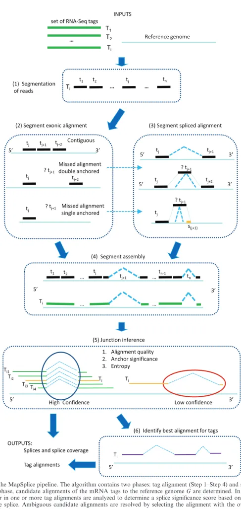
splices and to provide a basis for choosing the most likely alignment for each tag based on a combination of align-ment quality and splice significance. An overview of the algorithm can be found in Figure 1. The two phases are described in the following two sections.
Tag alignment
Letbe the set of tags and letmbe the tag length. A tag
T2has an ‘exonic alignment’ if it can be aligned in its entirety to a consecutive sequence of nucleotides in G. T has a ‘spliced alignment’ if its alignment toGrequires one or more gaps.
MapSplice identifies candidate tag alignments in three steps. First, tags are partitioned into consecutive short segments and an exonic alignment to Gis attempted for each segment. In the second step, segments that do not have an exonic alignment are considered for spliced align-ment using a splice junction search technique that starts from neighboring segments already aligned. In the final step, segment alignments for a tag are merged to find can-didate overall alignments for each tag. The details of the steps follow next.
Step 1: partition tags into segments. Tags in of length
m are partitioned into n consecutive segments of lengthk wherekm=2. Typically k is 20–25 for tags of length 50 or greater. Askis decreased, the chance that a segment contains one or more splice junctions decreases correspondingly, but the chance for multiple spurious alignments of the segment increases. The segments making up a tag T are labeled t1,t2,. . .,tn where the
number of segmentsn¼ mk :
Step 2: exonic alignment of segments. Exonic alignment of segments can be performed using fast approximate aligners such as Bowtie (23), and BWA (24), or aligners with more general error tolerance models such as SOAP2 (25), BFAST (26) and MAQ (27). For each segmentti of
tagT, letnibe the number of possible exonic alignments of
ti to the genome, determined using one of the algorithms
mentioned above with an error tolerance of k
mismatches. When ni¼1 the segment has a unique
exonic alignment. When ni>1 the segment has multiple
alignments, each of which is considered in the subsequent steps.
Step 3: spliced alignment of segments. Ifni¼0, segmentti
does not have an exonic alignment. One possible reason is that it may have a gapped alignment crossing a splice junction. In general, if the minimum exon length is at least 2k, then for every pair of consecutive segments in
Tat least one segment should have an exonic alignment. Therefore, the alignment of segment ti is localized to the
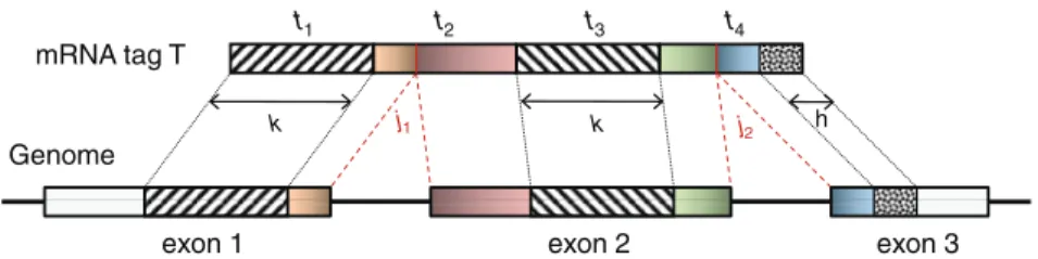
alignments of its neighbors. The following two techniques are used to find a spliced alignment for segments, and are illustrated in Figure 2.
If ti1 and ti+1 both have exonic alignments, then we
perform a ‘double-anchored’ spliced alignment of ti for
all combinations of exonic alignments of ti1 and ti+1. If
only one neighboring segmenttjhas an exonic alignment,
algorithm to predict splice junctions from a training set of positive controls (20). The TopHat algorithm con-structs candidate splice junctions by pairing candidate exons and evaluating the alignment of reads to such candidates (21). SpliceMap is another method that uses splice site flanking bases in locating potential splice sites(22).
WeintroducetheMapSplice algorithmtodetectsplice junctionswithout any dependence on splicesite features. This enables MapSplice to discover non-canonical junc-tions and other novel splicing events, in additional to the more common canonical junctions. MapSplice can be generally applied to both short and long RNA-seq reads. In addition, MapSplice leverages the quality and diversity of read alignments that include a given splice to increase specificity in junction discovery. As a result, MapSplice demonstrates high specificity and sensitivity. Performance results are established using synthetic data setsandvalidatedexperimentally.
We haveusedMapSplice to investigatesignificant dif-ferencesinalternativesplicing betweena setofbasaland luminal breastcancer tissues. Experimentalvalidation of 20exonskipping eventsbyquantitativeRT–PCR(qRT– PCR) correctly identified isoform proportions that are highly correlated (Pearson’s correlation=0.86) with theirestimates basedon splicejunctions. Splicejunctions also recapitulated the difference between molecular subtypesof breastcancer. Ona globallevel,the propor-tion of splice junctions in various categories of alterna-tive splicing was concordant with a previous RNA-seq study.
MATERIALSAND METHODS
ThegoalofMapSpliceistofindtheexonsplicejunctions present in the sampled mRNA transcriptome, and to determine the most likely alignment of each mRNA sequencetagtoareferencegenome.Eachtagcorresponds to a number of consecutive nucleotides read from an mRNA transcript, where the length of the tag is determined by the protocol and the sequencing technol-ogy.Forexample,theIlluminaGenomeAnalyzerIIx gen-eratesover20Mtagsof sizeupto 100bp persequencing lane.
MapSpliceoperatesintwophasestoachieveitsgoal.In the ‘tag alignment’ phase, candidate alignments of the mRNA tags to the reference genome G are determined. Tagswithacontiguousalignmentfallwithinanexonand canbemappeddirectlytoG,buttagsthatincludeoneor more splice junctions require a gapped alignment, with each gap corresponding to an intron spliced out during transcription. Since multiple possible alignments may be found,theresult ofthisphaseis,ingeneral,a setof can-didatealignmentsforeachtag.
then we perform a ‘single-anchored’ alignment starting from thenj possible alignments oftj.
(a) Double-anchored spliced alignment: the spliced alignment of ti to the genomic interval between
anchors ti1 and ti+1 need only consider the k+1
possible positions of the splice junction x within ti
and minimize alignment mismatch.
Formally, the ‘Hamming distance’ DHðS,TÞ between
two equal length sequences SandT is defined as the number of corresponding positions with mismatching bases. We define the spliced alignment between the segment t½1:k and the genomic intervalG½i:j as
spliced-alignðt½1:k,G½i:jÞ ¼
min arg1x<kDHðt½1:x,G½i:i+x1Þ
+DHðt½x+1:k,G½j ðkxÞ+1:jÞ
which yields the optimal position x of the splice junction int that gives the best spliced alignment to the given genomic interval. The splice junction x
defines the intron asG½i+x1:j ðkxÞ+1:
To find the spliced alignment for ti between
two aligned segments, let gi1 and gi+1 be the
leftmost genomic coordinates in the alignment of
ti1 and ti+1, respectively, and compute
spliced–alignðt½1:k,G½gi1+k:gi+11Þ:
In case the alignment cost for the splice junction exceeds the error tolerance threshold k, the
align-ment for ti fails. If there exists more than one
splice junction position with minimum cost for ti,
multiple alignments are recorded for ti:
(b) Single-anchored spliced alignment: in the case of a single anchor ti1 upstream of the unaligned ti, we
conduct a search for si, theh-base suffix ofti in the
genomic region downstream from ti1: Similarly, in
the case of a single anchor ti+1 downstream from ti,
the search is for the h-base prefix pi of ti in the
region upstream from ti+1: In either case this search
is limited in range by a parameter D, the maximum intron size for single anchor search, typically set to 50 000 bp.
All single anchored alignments can be resolved with a single traversal of (the expressed portion of) the genome using a sliding window of size D. An h-mer index is maintained during this traversal, mapping occurrences of an h-mer pi to the downstream
anchorti+1 within distance D and occurrences of an h-mer si to the upstream anchor ti1 within distance D. As the window moves, new entries are added as anchors come within range, and old entries are deleted as anchors fall out of range.
When the h-mer at the current coordinate c in the genome scan is mapped to a downstream segment
ti+1, spliced-alignðt½1:k,G½c:gi+11Þ gives the
best spliced alignment which is recorded if it is within the segment error threshold "k. Similarly,
when the h-mer is mapped to an upstream segment
ti1, we record spliced-alignðt½1:k,G½gi1+k:c+hÞif
it is within the segment error thresholdk.
(c) Spliced alignment in the presence of small exons: if an exon shorter than 2kis included in a transcript, it is possible that two adjacent segments ti and ti+1
both include a splice junction so that neither can be aligned continuously within an exonic region. If the exon is shorter than k, even a single segment might include more than one splice junction. The following approach allows us to detect exons with size less than 2k.
Assume S is a sequence of one or two missed segments between two anchors ½a,b that cannot be successfully aligned in the previous steps, potentially due to short exons. We divideS into a sequential set ofh-mers and indexS with theseh-mers. By extend-ing the sequential scan of the genome used in single-anchored spliced alignment,h-mers on the ref-erence genome in ½a,b can all be searched simultan-eously. When a match exists, two double-anchored spliced alignments will be performed: one is between a and the 50-site of the h-mer alignment;
and the other is between the 30-site of h-mer
align-ment and b.
According to the pigeon-hole principle, if the exon is no shorter than 2h, one of the h-mers in the un-aligned segments will fall within an exon and thus trigger the subsequent spliced alignments. Therefore, this method is guaranteed to detect small exons longer than 2h and possibly detect shorter exons. The typical h-mer size is 6–8 bps. When exons are shorter than 2h, the chances of finding a spliced alignment decrease. Reducing h
will lead to an increasing number of spurious matches that will be difficult to filter out.
Genome mRNA tag T
t1 t2 t3 t4
k j1 k j h
2
3 n o x e 2
n o x e 1
n o x e
Figure 2. A portion of an mRNA transcript sampled by tagTconsists of the 30end of exon 1, all of exon 2 and the 50end of exon 3.Tis split into segmentst1,. . .,tneach of lengthkto identify the alignment ofTto the genome. Provided no exon has a length less than 2knucleotides, at least one
of every two consecutive segments must have an exonic alignment. In this example withn¼4,segmentst1andt3have exonic alignment. Segmentt2 has spliced alignment; the splice junctionj1 can be easily discovered using the double-anchor search method starting fromt1 andt3. The spliced
Letibe the set of alignments for segmenttiand when
0<ni, let ji be the j-th alignment of ti, where 1in
and 1jni. In principle there exist Qni¼1ni different
combinations of alignments, but most can be ruled out by a simple coherence test based on contiguity of consecu-tive segment alignments.
Two adjacent segmentstiandti+1with exonic alignment
that are not contiguous on the genome are checked for a splice junction between the two segments using the double-anchored spliced alignment method. This proced-ure also corrects inaccurate splice points due to the error tolerance in the alignment oftiandti+1.
For each assembly of segments that yields a candidate alignment for T, we compute its ‘mismatch score’, a modified Hamming distance betweenTand its alignment to the genomeGT.
The mismatch score takes into account base call qualities when available. A poor quality base call can improve the score when associated with a mismatched base, but can also decrease the score when associated with a matched base (28). The base call quality for a given base x in the overall alignment of a tag T can be converted to a probabilityp thatxwas called incorrectly, and so the expected mismatch sðx,yÞin the alignment of basexto basey in the genome is given by
sðx,yÞ ¼ ð1pÞ=fx, x¼y
p=ð1fxÞ, x6¼y
ð1Þ
wherefxis the probability of basexin the background
dis-tribution of nucleotides. We assume a uniform distribu-tion for nucleotides hencefx¼1=4 for allx. Thus, given a
proposed alignment of T¼b1. . .bm and GT¼gi1. . .gim
andpithe probability that nucleotidebi was called
incor-rectly, the expected mismatch is
E½mismatchðT,GTÞ ¼j¼1,msðbj,gijÞ:
The candidate alignment is retained if
E½mismatchðT,GTÞ k, otherwise it is discarded. Note
that while each segment was aligned allowing "k
mismatches, the overall tag alignment only allows a total of k expected mismatches. We define the quality of the
alignment to bekE½mismatchðT,GTÞ: Splice junction inference
Splice junction alignments introduce a multiplicity of ways in which a tag may be split into pieces, each of which may be separately aligned to the genome. For a given tag, at most one of these is the true alignment. Splice inference leverages the extensive sampling of splice junctions by tags to compute a junction quality that can be used to distin-guish true splice junctions from spurious splice junctions and to determine the best alignment among the remaining candidate alignments of a tag.
Step 5: splice junction quality. For a given splice
J¼ ðJd,JaÞ, where Jd is the last coordinate of the donor
exon andJais the first coordinate of the acceptor exon, we
consider the setAðJÞof tags that include a splice junction for J in a candidate alignment. We define two statistical measures on AðJÞ: the ‘anchor significance’ sðAðJÞÞ,
determined by the alignment in AðJÞ that maximizes sig-nificance as a result of long anchors on each side of the splice junction, and the ‘entropy’hðAðJÞÞ,measured by the diversity of splice junction positions inAðJÞ:
(i) Anchor significance of a splice junction: a tag that includes a splice junction has some number of con-tiguous bases aligned on either side of the splice site. An alignment with a short anchor on one side has low confidence, since we expect it to be easy to find other occurrences of the sequence of nucleotides found in the short anchor each of which might equally well be the correct target. We define the anchor significance of a splice J in a tag T2AðJÞ
as follows. Let Tp be the maximal contiguous
sequence of bases in T with exonic alignment ending at coordinate Jd in the genome, and let Tq
be the maximal contiguous sequence of bases in T
with exonic alignment starting from coordinate Ja:
These are the two anchors, each of which has at least one alignment (the one in T). The expected number of alignments in the genome for an anchor Ta is therefore given by
EðTaÞ ¼ 1+ D
4jTaj ifTafound by single anchor search
1+N
4jTaj otherwise
Here, we model the genome as a sequence of inde-pendent random variables with uniform distribution over A, C, T, G, so that the chance that a length n
sequence aligns at a given coordinate is simply 4n. For double-anchor alignments, the search space is effectively the entire genome of lengthN. For single anchor alignments, we only consider occurrences within distanceD.
Since we assume that only one of the potential alignments is correct and the rest are spurious, the chance of a spurious alignment of anchor
Ta is 0<1EðTaÞ1 <1: Thus the
log-transformed significance of anchor Ta is
sðTaÞ ¼ log2ð1EðTaÞ1Þ: The anchor alignment
of junction J in T is only as significant as the anchor with least confidence, hence is
sTðJÞ ¼minðsðTpÞ,sðTqÞÞ:
The anchor significance of junctionJover all occur-rences in T2AðJÞ is the occurrence with greatest anchor significance:
sðAðJÞÞ ¼ max
T2AðJÞsTðJÞ
(ii) Entropy: in principle, the RNA-seq protocol samples each transcript uniformly, so that the position of a true splice junction J within AðJÞ is expected to be uniformly distributed on 1::m,
provided the sampling is sufficiently deep and the
Step 4: merging segment alignments. The assembly of a completetag alignmentfrom individual alignmentsofits segments is straightforward if each segment is aligned uniquely and connects to its neighboring segments without a gap. However, a given segment ti may be
splice junction is not too close to the end of the transcript. To measure the uniformity of the sampling, we apply Shannon maximum entropy to the distribution of splice junction positions in AðJÞ
for splice J.Let pi with 1i<mbe the frequency
of occurrence of a splice junction J at position i
within AðJÞ: The Shannon entropy can be measured as
hðAðJÞÞ ¼ X 1i<m
pilog2pi
The higher the Shannon entropy, the closer the dis-tribution is to uniform, and therefore the higher the chance that the junction is part of some transcript that was sampled uniformly.
(iii) Combined Metric: the combined metric pðJÞ is the posterior probability that junction J is a true junction determined using Bayesian regression. The observed data of pðJÞ are the entropy and anchor significance ofJwithin AðJÞand the average quality of read alignments that include J.
pðJÞ ¼sðAðJÞÞ+hðAðJÞÞ+qðAðJÞÞ+"
We apply linear regression to obtain the best config-uration of , and that achieves the maximum sensitivity and specificity in junction classification.
Step 6: best alignment for tags. For each tagT, we select the candidate alignmentTGthat achieves the highest score
when combining alignment quality from Step 4 and junction quality from Step 5.
Synthetic data generation for validation
To evaluate the sensitivity and specificity of MapSplice, we generated synthetic data sets of tags derived from transcripts cataloged in the Alternative Splicing and Transcript Diversity (ASTD) database (29).
This database collects full-length transcripts illustrating alternative splicing events in genes from human, mouse and rat. A synthetic ‘transcriptome’ is generated by randomly selecting genes and expression levels according to an empirical distribution of tags per gene observed in Ref. (1). Within a gene, transcripts are selected at random following various submodels that determine expression level of individual transcripts relative to the overall gene. The synthetic transcriptome characterized in this fashion is then sampled to yield two synthetic RNA-seq data sets. The noise-free data set samples the transcripts exactly and the resultant tags align to the reference genome exactly to model single-nucleotide variations in the data base tran-scripts. The noisy data set introduces mutations into base calls following empirical Illumina base call quality profiles. The resulting data sets mimic the observed distri-bution of errors in tags in Ref. (30).
Experimental validation by qRT–PCR
Total RNA isolated from MCF-7 and SUM-102 cells was reverse transcribed using the High-Capacity cDNA Reverse Transcription Kit with RNase inhibitor
(Applied Biosystems, Foster City, CA, USA) as per manu-facturer’s instructions. Relative expression levels of the transcripts of interest were determined by qRT–PCR on the Applied Biosystems 7300 Real Time PCR System with premade or custom TaqMan Gene Expression Assays (Applied Biosystems, Foster City, CA, USA) containing primers flanking the splice sites of interest and FAM/ MGB-labeled oligonucleotide probes. PCR reactions were carried out as per manufacturer’s instructions. cDNA equivalent to 100 ng of total RNA was amplified with 1ml of TaqMan assay in Gene Expression master mix in a total volume of 20ml. Each assay was performed in triplicate. Thermal Cycling conditions were as follows: 50C for 2 min, 95C for 10 min, 40 cycles of 95C for
15 s and 60C for 1 min. Ct values were determined in
the manufacturer’s software, data was further analyzed in Excel utilizing comparative Ct method. For compari-sons of relative expression levels between the two cell lines,
Ct values for the transcripts of interest were first normalized to those of HPRT1.
RESULTS
Junction inference
We constructed a synthetic noise-free RNA-seq data set with 20M 100 bp tags sampling 46 311 distinct transcripts from the ASTD. The tags were aligned to the reference genome (hg18) using the MapSplice algorithm steps 1–4 with k¼25, h¼8 andk¼1: To establish the training
data set containing both true and false junctions, no re-strictions on splice site flanking sequences or maximum intron size were enforced.
We randomly selected 10K true junctions and 10K false junctions as a training set and analyzed the three different junction classification metrics utilized in Step 5 of MapSplice: alignment quality entropy and anchor signifi-cance, as well the combined metric obtained by linear regression of the first three metrics. Five-fold cross-validation was applied to avoid sample bias in training. The ROC curve that illustrates the sensitivity and specificity of each metric is shown in Figure 3. The combined metric (solid green curve) offers better classifi-cation results than individual metrics simply because indi-vidual metrics only capture one property of a junction. At the best point, the combined metric achieves a true-positive rate of 96.3% and false-positive rate of 8%. We also compared the results with one of the most commonly used metrics: junction coverage (the number of tags aligned to a junction). In many studies, a junction is considered to be true if at least three tags are aligned to the junction. However, as shown in Figure 3, coverage (solid red curve) is the least reliable metric and yields the worst performance in terms of junction classification.
SpliceMap including minimum anchor (extension) of 10 bp and no multiple alignments within a 400 kb region improved its specificity with some tradeoff in sensitivity in 100 bp tags. MapSplice performed best in both categories by detecting more true-positive junctions and fewer false-positive junctions.
Due to the incompleteness of SpliceMap’s output (tag alignments were not generated), we limit the more comprehensive comparison to TopHat and MapSplice. We investigated the sensitivity and specificity in splice in-ference as a function of tag length and sampling depth. We generated synthetic data sets to study the effect of these variations on junction discovery. In the synthetic data set, we have ground truth junctions and know their actual coverage, i.e. the number of tags spanning each junction. Two measures were used to evaluate the algorithms. The ‘sensitivity’ is the ratio of the total number of true junc-tions discovered to the total number of juncjunc-tions sampled in the synthetic data. The ‘specificity’ is the ratio of the total number of true junctions discovered over the total number of discovered junctions. Since coverage of a junction is essential for the junction to be discovered, we plot sensitivity and specificity at coveragex as the sensi-tivity and specificity for all junctions with coverage x
or greater, as shown in Figure 4. We also show the re-covered ‘coverage ratio’ for junctions identified as true in Figure 5.
Effect of noise. In the first experiment, we constructed the error-free and noisy versions of a 100 bp synthetic RNA-seq data sets of 20M tags as described above. MapSplice and TopHat were run on both data sets and given the same error tolerance of 4% (k¼4). Figure 5A
and B shows that performance was only impaired at low coverage. When coverage is high, the sensitivity is similar despite the presence of errors. Specificity is more affected, but also converges to similar performance when coverage is high. With low coverage, more spurious junctions were discovered in the data set with error than the one without. Comparing MapSplice with TopHat, MapSplice has higher sensitivity and specificity in identifying junctions in both data sets. Specificity is substantially higher even at low coverage.
Effect of tag length. In the second experiment, we generated a synthetic data set of 20M 100 bp tags and created two additional data sets by selecting a 50 and
0 0.1 0.2 0.3 0.4 0.5 0.6 0.7 0.8 0.9 1
0 0.1 0.2 0.3 0.4 0.5 0.6 0.7 0.8 0.9 1
False positive rate
True positive rate
alignment quality anchor confidence entropy
coverage combined
Figure 3. ROC curves for junction classification. A synthetic data set of 20M 100 bp tags was generated from transcripts selected from the ASTD database. 10K true-positive junctions and 10K false-positive junctions were selected as training data sets. Five different metrics were evaluated. They include (i) alignment quality; (ii) anchor signifi-cance; (iii) entropy; (iv) coverage; and (v) combination of metrics (i–iii). The red cross in each curve marks the point with best balance of sen-sitivity and specificity.
Table 1. Comparison of TopHat (21), SpliceMap (22) and MapSplice on two synthetic data sets with tags of length 50 and 100 bp, respectively
Data set Method Performance Junction discovery
Time Peak Mem. Total True False
50 bp TopHat (1.0.12) 50 min <4 GB 85 356 76 486 8870
SpliceMap (C++3.0) 13 h 9.3 GB 88 807 87 205 1602
MapSplice 25 min <4 GB 88 180 87 330 750
100 bp TopHat (1.0.12) 3 h 40 min <4 GB 100 012 90 720 9292
SpliceMap (C++3.0) 41 h 12 GB 91 259 89 991 1268
MapSplice 1 h 50 min <4 GB 94 112 92 849 1263
Both data sets have 20 million tags.
The best values in each comparison are shown in bold.
robustnessof the parameters and their sensitivity to tag length and sampling depth are included in the SupplementaryData.
Sensitivityandspecificityofspliceinference
ThreeprogramsthatmapsplicejunctionsusingRNA-seq data were compared, MapSplice, TopHat (1.0.12) and SpliceMap (C++, v3.0, 15 April 2010). We applied all three algorithms to two representative synthetic data sets. One was a data set with 20M tags of length50bp. Theotherwasadatasetwith20M100bptags.Forboth MapSpliceandTopHat,wesetk¼25,h¼8andk¼1.
75 bp random subsequences of the 100 bp tags, respec-tively. Both MapSplice and TopHat were applied to these data sets with maximum percentage of mismatches as 4% of the tag length. The result is shown in Figure 5C
and D. In general, for both TopHat and MapSplice, longer tags not only improve the sensitivity but also improve the specificity of the junction discovery. In com-parison, MapSplice has higher sensitivity for all three tag
100 101 102
0.9 0.91 0.92 0.93 0.94 0.95 0.96 0.97 0.98 0.99 1
Junction coverage
Sensitivity
tophat error=0 tophat error>0 mapsplice error=0 mapsplice error>0
100 101 102
0.9 0.91 0.92 0.93 0.94 0.95 0.96 0.97 0.98 0.99 1
Junction coverage
Specificity
tophat error=0 tophat error>0 mapsplice error=0 mapsplice error>0
100 101 102
0.8 0.82 0.84 0.86 0.88 0.9 0.92 0.94 0.96 0.98 1
Junction coverage
Sensitivity
tophat 50bp tophat 75bp tophat 100bp mapsplice 50bp mapsplice 75bp mapsplice 100bp
100 101 102
0.8 0.82 0.84 0.86 0.88 0.9 0.92 0.94 0.96 0.98 1
Junction coverage
Specificity
tophat 50bp tophat 75bp tophat 100bp mapsplice 50bp mapsplice 75bp mapsplice 100bp
100 101 102
0.9 0.91 0.92 0.93 0.94 0.95 0.96 0.97 0.98 0.99 1
Junction coverage
Sensitivity
tophat 10M tophat 20M mapsplice 10M mapsplice 20M
100 101 102
0.9 0.91 0.92 0.93 0.94 0.95 0.96 0.97 0.98 0.99 1
Junction coverage
Specificity
tophat 10M tophat 20M mapsplice 10M mapsplice 20M
A B
C D
E F
lengths. The difference in sensitivity is more pronounced in junctions with low coverage, where junction discovery is most difficult.
Effect of sampling depth. In the final experiment, we generated two 100 bp data sets with a different number of tags: 10M and 20M, respectively. Doubling the sampling depth does not double the specificity of junctions, but it does improve the sensitivity. Doubling the depth has a negative effect on specificity, especially in the low coverage areas. This is mostly because increasing the number of tags sampled from a fixed number of transcripts increases the chances for a repeated tag, especially one with a high error rate, to be incorrectly aligned on the genome.
Breast cancer transcriptomes
We performed cDNA sequencing to obtain about 25 million tags of length 75 bp for four primary breast tumors and replicate samples for two breast cancer cell lines. In total, four samples correspond to the basal subtype of breast cancer, and four samples correspond to the luminal subtype. We applied both MapSplice and TopHat to detect splice junctions using the same param-eter settings employed with the synthetic data sets. The mapping result is shown in Table 2. In summary, between 10% and 16% of the tags in each sample include splice junctions in their alignment. Over 77% of these canonical junctions were confirmed by known tran-scripts in GenBank, which represented between 6% and 11% more confirmed junctions than TopHat. MapSplice
identified 24213173 semi-canonical junctions, much less than the number reported by TopHat. But for both sets, very similar sets of junctions are known, which suggests that MapSplice has a higher specificity for non-canonical splice junctions.
MapSplice reported between 1157 and 1967 non-canonical splice junctions, of which 5–8% were con-firmed in known GenBank transcripts. While TopHat reported up to 5944 non-canonical junctions, none of them were confirmed in GenBank transcripts. Since the TopHat program does not search for non-canonical junc-tions, this result might be an artifact. We found 9205 genes that showed evidence of alternative splicing, ranging from 7371 to 8942 genes per tumor. There were 420 to 430 ca-nonical junctions identified by MapSplice within 2 bp of a known semi-canonical or non-canonical junction. For almost all of them, the tags aligned to the canonical junction have fewer mismatches than if they were aligned to the nearby non-canonical or semi-canonical junction. Such findings suggest that there exist errors in the current database and RNA-seq data might be able to correct these errors.
MapSplice detected the expected proportion of alterna-tive splicing categories, even though it did not rely on a database of transcript annotations. We investigated how many alternative splicing events could be detected at dif-ferent minimum thresholds for the minor transcript isoforms (Table 3). For instance, at a cutoff of two or more tags per splice junction, MapSplice detected between 7535 and 8270 alternative splicing events in
0 0.2 0.4 0.6 0.8 1 1.2 1.4 1.6 1.8 2
1 2 4 8 16 32 64 128 256 512 1024 2048
Junction coverage
Percentage of recovered reads
0 0.2 0.4 0.6 0.8 1 1.2 1.4 1.6 1.8 2
1 2 4 8 16 32 64 128 256 512 1024 2048
Junction coverage
Percentage of recovered reads
A B
each tumor. These events comprised: 34.5% skipped exons; 30.3% alternative 50-sites; 33.8% alternative
30-sites; and 1.4% mutually exclusive exons. A previous
RNA-seq study across 10 different tissues and 10 different cell lines (1) reported similar values: 35% skipped exons; 28% alternative 50-sites and first exons; 31% alternative
30-sites, last exons and UTRs; and 4% mutually exclusive
exons. The high concordance between these two studies further suggested that the MapSplice alignments were highly accurate.
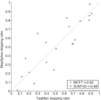
We randomly selected skipped exon events for the ex-perimental validation of MapSplice alignments to splice junctions. We calculated the proportion of splice junction tags aligning to the skipped exon isoform, and then compared this to the total number of splice junction tags aligning to either the skipped exon isoform or the included exon isoform (Figure 6). We compared these calculations with the splicing ratio determined by qRT–PCR in the MCF-7 and SUM-102 cell lines. With a Pearson’s correlation of 0.84 across these 20 events, MapSplice achieved very high accuracy for splice junction counting.
We identified 12 exon skipping events with significant differences between the basal and luminal subtypes. For instance, NUMB is an adaptor protein in the Notch and Hedgehog pathways with a potential skipped exon in an N-terminal PTB domain, as well as another skipped exon in a C-terminal proline-rich region (31). While all breast cancer samples had similar skipping ratios for the PTB domain exon, we detected significant differences for the skipped exon in the proline-rich region. This longer isoform had exon inclusion ratios ranging 45–78% in the luminal samples, compared with 16–22% of the basal
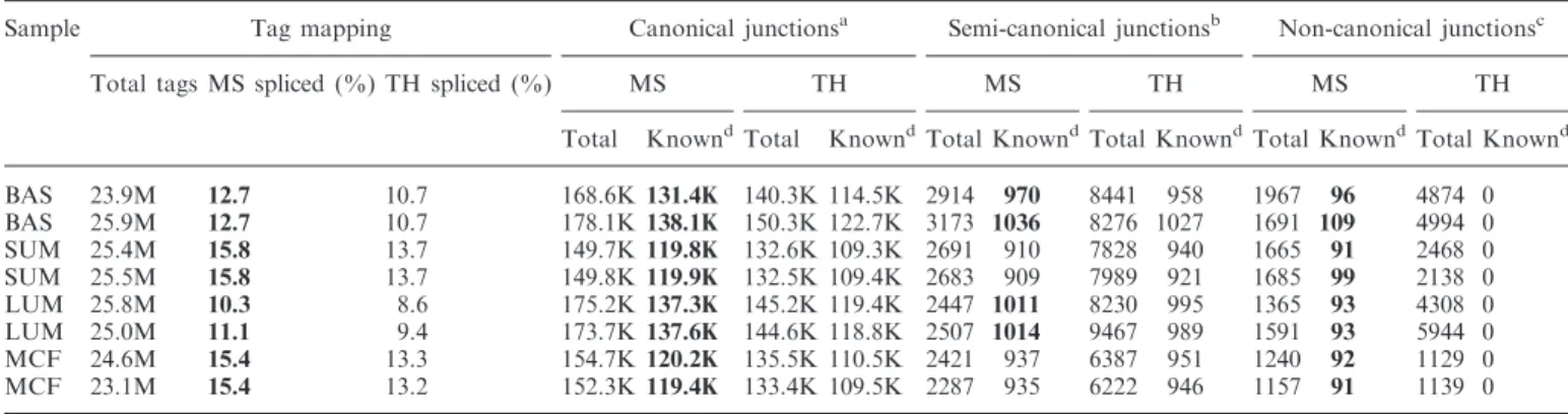
Table 2. Tag mapping and splice junction detection results on eight breast cancer samples: two basal (BAS) primary tumors, two SUM-102 (SUM) cell lines, two luminal (LUM) primary tumors and two MCF-7 (MCF) cell lines
Sample Tag mapping Canonical junctionsa Semi-canonical junctionsb Non-canonical junctionsc
Total tags MS spliced (%) TH spliced (%) MS TH MS TH MS TH
Total KnowndTotal KnowndTotal KnowndTotal KnowndTotal KnowndTotal Knownd
BAS 23.9M 12.7 10.7 168.6K131.4K 140.3K 114.5K 2914 970 8441 958 1967 96 4874 0 BAS 25.9M 12.7 10.7 178.1K138.1K 150.3K 122.7K 3173 1036 8276 1027 1691 109 4994 0 SUM 25.4M 15.8 13.7 149.7K119.8K 132.6K 109.3K 2691 910 7828 940 1665 91 2468 0 SUM 25.5M 15.8 13.7 149.8K119.9K 132.5K 109.4K 2683 909 7989 921 1685 99 2138 0 LUM 25.8M 10.3 8.6 175.2K137.3K 145.2K 119.4K 2447 1011 8230 995 1365 93 4308 0 LUM 25.0M 11.1 9.4 173.7K137.6K 144.6K 118.8K 2507 1014 9467 989 1591 93 5944 0 MCF 24.6M 15.4 13.3 154.7K120.2K 135.5K 110.5K 2421 937 6387 951 1240 92 1129 0 MCF 23.1M 15.4 13.2 152.3K119.4K 133.4K 109.5K 2287 935 6222 946 1157 91 1139 0
MapSplice (MS) detected 177 875 splice junctions occurring in at least two tags in any of the breast tumors or cell lines. Of the tags, 10–16% in each sample contained splice junctions. MapSplice detected 149.7K–178.1K canonical junctions, among which about 109.3K–122.7K are confirmed by known transcripts in GenBank. In general, MapSplice detected 10K–18K more canonical junctions than TopHat (TH). MapSplice identified 2421–3173 semi-canonical junctions, far fewer than the number reported by TopHat. But in both sets, a very similar subset of junctions are known. There are 91–99 non-canonical junctions known out of the 1157–1967 non-canonical junctions reported by MapSplice. While TopHat did report up to 5944 non-canonical junctions, none of them are confirmed.
aFlanked by GT-AG. b
Flanked by AT-AC or GC-AG. cOther flanking dinucleotide. d
A junction is known if it is included in at least one transcript in GenBank.
Table 3. A survey of alternative exon splicing events identified with MapSplice junctions
Coverage Alternative exon events Mutual Excl.
Sample Skipped Exon Alt. Start Alt. End
1 BAS 6880 6700 7474 442
BAS 7365 7611 8005 454 SUM 5574 5690 6359 353 SUM 5491 5701 6451 337 LUM 6523 7326 7777 387 LUM 6321 6928 7625 355 MCF 6776 6338 7350 472 MCF 6352 6063 7083 444
2 BAS 2726 2144 2564 101
BAS 2941 2529 2689 111 SUM 2271 2098 2347 103 SUM 2277 2096 2359 95 LUM 2599 2542 2574 95 LUM 2333 2031 2387 86 MCF 2949 2410 2778 129 MCF 2669 2331 2588 109
5 BAS 651 476 614 26
BAS 718 522 641 23
SUM 644 538 643 25
SUM 623 528 656 25
LUM 618 538 582 22
LUM 503 386 528 21
MCF 815 686 780 30
MCF 757 656 735 22
samples (Figure 7). We expect that as more samples are sequenced, we will have more statistical power to identify alternative splicing events that can distinguish between cancer subtypes.
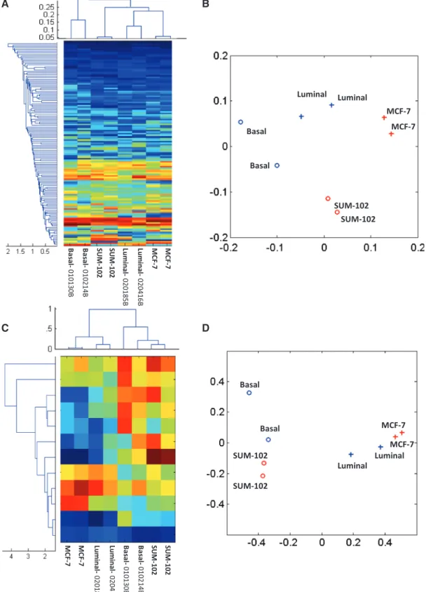
We investigated whether molecular subtypes of tumors may have different patterns of alternative splicing regard-less of their gene expression levels. We selected 129 single exon skipping events that were detected by at least three tags in each tumor. The matrix of splicing ratios was then hierarchically clustered, with each row representing a distinct splicing event and each column representing a single tumor (Figure 8). Notably, the two primary breast tumors from the luminal subtype clustered together, as did the two primary breast tumors from the basal subtype. The breast cancer cell lines clustered in between the primary tumors, which indicates that these cell lines resemble their primary tumors of origin, but also share some major differences in splicing. Principal components analysis on these splicing ratios reached similar conclu-sions: the first principal component distinguished cell lines from primary tumors, while the second principal component segregated luminal versus basal subtypes (Figure 8B and D).
Figure 7. Examples of alternative exon skipping events. The second exon in NUMB shows differential alternative splicing between two cancer subtypes. The exon skipping ratios in basal samples are70% while in luminal samples they are<50%.
0 0.1 0.2 0.3 0.4 0.5 0.6 0.7 0.8 0.9 1
0 0.1 0.2 0.3 0.4 0.5 0.6 0.7 0.8 0.9 1
TaqMan skipping ratio
MapSplice skipping ratio
MCF7 r=0.83 SUM102 r=0.88
A B
C D
>100 bp. With a processing power of 10 million reads (100 bp) per hour and peak memory usage below 4 GB, MapSplice can run on both desktop and servers with high efficiency.
Third, MapSplice incorporates a rigorous approach to increase specificity of the splice search, necessitated by the multiple ways in which some RNA-seq tags can find spliced alignments to the genome. By leveraging the deep sampling of the transcriptome in RNA-seq data sets, spurious splices can be discriminated from true splices. High specificity is critical as a typical RNA-seq data set can contain some evidence for hundreds of thou-sands of splices.
In this article, we have made a rigorous measurement of sensitivity and specificity of splice finding algorithms using realistic synthetic data sets. The performances are further assessed by experimental validation of results obtained from breast cancer samples. Using synthetic data sets, we determined that read lengths of 75 or 100 bp yield sig-nificantly better sensitivity and specificity for splice detec-tion than 50 bp data sets. We determined that splices can be found despite the presence of errors. Finally, we used synthetic data to calibrate several filtering criteria to achieve over 98% specificity and 96% sensitivity in the detection of splice junctions in the simulated data. These filtering criteria provided superior accuracy in our com-parisons to the TopHat (21) and SpliceMap (22) algorithms.
Several experimental lines of evidence also confirmed a high accuracy of the MapSplice algorithm’s splice junction alignments. First, the distribution of splice junctions in
various categories of alternative splicing are highly con-cordant with previous studies (Table 3). Second, experi-mental validation of 10 predictions by qRT-PCR correctly identified isoform proportions that are highly correlated (Pearson’s correlation = 0.86) with their estimates based on splice junctions. Third, hierarchical clustering of splicing ratios recapitulated known molecular subtypes of four breast tumors and two breast cancer cell lines. As sample size increases, we will achieve more power to identify candidate genes with significant differences in splicing isoform proportions between molecular subtypes of cancer.
This deep sequencing study represents the first survey of alternative splicing differences between cancer subtypes. At a sequencing depth of approximately 20 million reads with a length of 75 bp, we identified between 149 722 and 178 107 canonical splice junctions, as well as 3661 to 4884 semi-canonical and non-canonical splice junctions. Notably, we discovered that 19–22% of these splice junc-tions have not been previously observed in full-length transcripts in GenBank. Among these junctions, 15% connected two known exons, suggesting novel isoforms with exon skipping events.
We anticipate that tests between sample groups will be crucial to interpret data from large-scale transcriptome sequencing projects, such as the Cancer Genome Atlas. Future research efforts will be needed to distinguish splicing patterns that are enriched in a (potentially hetero-geneous) disease state, compared to the natural variation in alternative splicing within populations (5).
The reconstruction of full-length transcripts from short sequence reads is a challenging task, especially for low abundance transcripts. Splice junctions constitute the building blocks for these algorithms (19,32–35). We antici-pate that further advances in sequencing technologies, such as higher read depths and longer reads, will continue to improve these methods. Recent studies have combined both splice junction reads and exon reads to provide an integrated partitioning of alignments (36).
SUPPLEMENTARY DATA
Supplementary Data are available at NAR Online.
ACKNOWLEDGEMENTS
We wish to thank Zefeng Wang, Ben Berman, Corbin Jones, Oleg Evgrafov and the anonymous reviewers for their critical comments on the manuscript.
FUNDING
National Science Foundation (grant number 0850237 to J.L., J.N.M. and J.F.P.); National Institutes of Health (grant number CA143848 to C.M.P. and grant number P20RR016481 to J.L.); Alfred P. Sloan Foundation (to D.Y.C.). Funding for open access charge: National Institutes of Health (grant number CA143848).
Conflict of interest statement. None declared.
DISCUSSION
Accurate identification and quantification of transcript isoforms is crucial to characterize alternative splicing among different cell types. In addition, sequence variantsfoundwithin splicesitesor splicingenhancer se-quencesmayhavefunctionalconsequenceson alternative splicing. Thus, methods to accurately detect alternative splicing events will be necessary to determine whether thesesequencevariantsaffect thetranscriptisoform pro-portions.Sincecertainsplicejunctionscanunambiguously distinguish transcript isoforms, we have focused on increasing the accuracy of aligning splice junctions
denovo.Forthistask,wedevelopedanewsplicediscovery algorithm,MapSplice,thatmeetsthreegoals.
First, MapSplice performs a sensitive, complete and unbiasedsearchtofindsplicejunctionsusingapproximate sequence similarity that is not dependent on features or locationsofthesplicesites.Asaresult,thealgorithmcan be applied equally to RNA-seq data from well-studied model organisms and also data from organisms with sparse transcriptsannotations. The algorithm is capable of finding short-range as well as long-range and inter-chromosomal splices such as that might arise in genefusionand otherchimericsplicingeventsthatresult fromdamageto theDNA.
REFERENCES
1. Wang,E.T., Sandberg,R., Luo,S.J., Khrebtukova,I., Zhang,L., Mayr,C., Kingsmore,S.F., Schroth,G.P. and Burge,C.B. (2008) Alternative isoform regulation in human tissue transcriptomes. Nature,456, 470–476.
2. Luco,R.F., Pan,Q., Tominaga,K., Blencowe,B.J., Pereira-Smith,O.M. and Misteli,T. (2010) Regulation of alternative splicing by histone modifications.Science,327, 996–1000. 3. Andersen,L.B., Ballester,R., Marchuk,D.A., Chang,E.,
Gutmann,D.H., Saulino,A.M., Camonis,J., Wigler,M. and Collins,F.S. (1993) A conserved alternative splice in the von Recklinghausen neurofibromatosis (NF1) gene produces two neurofibromin isoforms, both of which have GTPase-activating protein activity.Mol. Cell. Biol.,13, 487–495.
4. Screaton,G.R., Bell,M.V., Jackson,D.G., Cornelis,F.B., Gerth,U. and Bell,J.I. (1992) Genomic structure of DNA encoding the lymphocyte homing receptor CD44 reveals at least 12 alternatively spliced exons.Proc. Natl Acad. Sci. USA,89, 12160–12164.
5. Kwan,T., Benovoy,D., Dias,C., Gurd,S., Provencher,C., Beaulieu,P., Hudson,T.J., Sladek,R. and Majewski,J. (2008) Genome-wide analysis of transcript isoform variation in humans. Nat. Genet.,40, 225–231.
6. Meyers,G.A., Day,D., Goldberg,R., Daentl,D.L., Przylepa,K.A., Abrams,L.J., Graham,J.M. Jr, Feingold,M., Moeschler,J.B., Rawnsley,E.et al. (1996) FGFR2 exon IIIa and IIIc mutations in Crouzon, Jackson-Weiss, and Pfeiffer syndromes: evidence for missense changes, insertions, and a deletion due to alternative RNA splicing.Am. J. Hum. Genet.,58, 491–498.
7. Pollock,P.M., Gartside,M.G., Dejeza,L.C., Powell,M.A., Mallon,M.A., Davies,H., Mohammadi,M., Futreal,P.A., Stratton,M.R., Trent,J.M.et al. (2007) Frequent activating FGFR2 mutations in endometrial carcinomas parallel germline mutations associated with craniosynostosis and skeletal dysplasia syndromes.Oncogene,26, 7158–7162.
8. Perou,C.M., Sorlie,T., Eisen,M.B., van de Rijn,M., Jeffrey,S.S., Rees,C.A., Pollack,J.R., Ross,D.T., Johnsen,H., Akslen,L.A.et al. (2000) Molecular portraits of human breast tumours.Nature,406, 747–752.
9. Dutt,A., Salvesen,H.B., Chen,T.H., Ramos,A.H., Onofrio,R.C., Hatton,C., Nicoletti,R., Winckler,W., Grewal,R., Hanna,M.et al. (2008) Drug-sensitive FGFR2 mutations in endometrial
carcinoma.Proc. Natl Acad. Sci. USA,105, 8713–8717. 10. Johnson,J.M., Castle,J., Garrett-Engele,P., Kan,Z., Loerch,P.M.,
Armour,C.D., Santos,R., Schadt,E.E., Stoughton,R. and Shoemaker,D.D. (2003) Genome-wide survey of human alternative pre-mRNA splicing with exon junction microarrays. Science, 302, 2141–2144.
11. Pan,Q., Shai,O., Misquitta,C., Zhang,W., Saltzman,A.L., Mohammad,N., Babak,T., Siu,H., Hughes,T.R., Morris,Q.D. et al. (2004) Revealing global regulatory features of mammalian alternative splicing using a quantitative microarray platform. Mol. Cell,16, 929–941.
12. Ule,J., Ule,A., Spencer,J., Williams,A., Hu,J.S., Cline,M., Wang,H., Clark,T., Fraser,C., Ruggiu,M.et al. (2005) Nova regulates brain-specific splicing to shape the synapse.Nat. Genet., 37, 844–852.
13. Castle,J.C., Zhang,C., Shah,J.K., Kulkarni,A.V., Kalsotra,A., Cooper,T.A. and Johnson,J.M. (2008) Expression of 24,426 human alternative splicing events and predicted cis regulation in 48 tissues and cell lines.Nat. Genet.,40, 1416–1425.
14. Pan,Q., Shai,O., Lee,L.J., Frey,J. and Blencowe,B.J. (2008) Deep surveying of alternative splicing complexity in the human transcriptome by high-throughput sequencing.Nat. Genet.,40, 1413–1415.
15. Mortazavi,A., Williams,B.A., McCue,K., Schaeffer,L. and Wold,B. (2008) Mapping and quantifying mammalian transcriptomes by RNA-Seq.Nat. Methods,5, 621–628.
16. Sultan,M., Schulz,M.H., Richard,H., Magen,A., Klingenhoff,A., Scherf,M., Seifert,M., Borodina,T., Soldatov,A., Parkhomchuk,D. et al. (2008) A global view of gene activity and alternative splicing by deep sequencing of the human transcriptome.Science, 321, 956–960.
17. Mereau,A., Anquetil,V., Cibois,M., Noiret,M., Primot,A., Vallee,A. and Paillard,L. (2009) Analysis of splicing patterns by pyrosequencing.Nucleic Acids Res.,37, e126.
18. Xing,Y., Yu,T., Wu,Y.N., Roy,M., Kim,J. and Lee,C. (2006) An expectation-maximization algorithm for probabilistic
reconstructions of full-length isoforms from splice graphs. Nucleic Acids Res.,34, 3150–3160.
19. Jiang,H. and Wong,W.H. (2009) Statistical inferences for isoform expression in RNA-Seq.Bioinformatics,25, 1026–1032.
20. De Bona,F., Ossowski,S., Schneeberg,K. and Ratsch,G. (2008) Optimal spliced alignments of short sequence reads.
Bioinformatics,24, i174–i180.
21. Trapnell,C., Pachter,L. and Salzberg,S.L. (2009) TopHat: discovering splice junctions with RNA-Seq.Bioinformatics,25, 1105–1111.
22. Au,K., Jiang,H., Lin,L., Xing,Y. and Wong,W.H. (2010) Detection of splice junctions from paired-end RNA-seq data by SpliceMap.Nucleic Acids Res.,2010, doi:10.1093/nar/gkq211. 23. Langmead,B., Trapnell,C., Pop,M. and Salzberg,S.L. (2009)
Ultrafast and memory-efficient alignment of short DNA sequences to the human genome.Genome Biol.,10, R25. 24. Li,H. and Durbin,R. (2009) Fast and accurate short read
alignment with Burrows-Wheeler transform.Bioinformatics,25, 1754–1760.
25. Li,R., Yu,C., Li,Y., Lam,T.W., Yiu,S.M., Kristiansen,K. and Wang,J. (2009) SOAP2: an improved ultrafast tool for short read alignment.Bioinformatics,25, 1966–1967.
26. Homer,N., Merriman,B. and Nelson,S.F. (2009) BFAST: an alignment tool for large scale genome resequencing.PLoS ONE, 4, e7767.
27. Li,H., Ruan,J. and Durbin,R. (2008) Mapping short DNA sequencing reads and calling variants using mapping quality scores.Genome Res.,18, 1851–1858.
28. Malde,K. (2008) The effect of sequence quality on sequence alignment.Bioinformatics,24, 897–900.
29. Koscielny,G., Le Texier,V., Gopalakrishnan,C., Kumanduri,V., Riethoven,J.J., Nardone,F., Stanley,E., Fallsehr,C., Hofmann,O., Kull,M.et al. (2009) ASTD: the Alternative Splicing and Transcript Diversity database.Genomics,93, 213–220.
30. Kircher,M., Stenzel,U. and Kelso,J. (2009) Improved base calling for the Illumina Genome Analyzer using machine learning strategies.Genome Biol.,10, R83.
31. Gulino,A., Di Marcotullio,L. and Screpanti,I. (2010) The multiple functions of Numb.Exp. Cell Res.,316, 900–906.
32. Heber,S., Alekseyev,M., Sze,S.H., Tang,H. and Pevzner,P.A. (2002) Splicing graphs and EST assembly problem.Bioinformatics, 18(Suppl. 1), S181–S188.
33. Xing,Y. and Lee,C. (2008) Reconstruction of full-length isoforms from splice graphs.Methods Mol. Biol.,452, 199–205.
34. Birol,I., Jackman,S.D., Nielsen,C.B., Qian,J.Q., Varhol,R., Stazyk,G., Morin,R.D., Zhao,Y., Hirst,M., Schein,J.E.et al. (2009) De novo transcriptome assembly with ABySS. Bioinformatics,25, 2872–2877.
35. Zheng,S. and Chen,L. (2009) A hierarchical Bayesian model for comparing transcriptomes at the individual transcript isoform level.Nucleic Acids Res.,37, e75.