Stochastic Processes and their Applications 123 (2013) 156–190
www.elsevier.com/locate/spa
Law of large numbers for non-elliptic random walks in
dynamic random environments
F. den Hollander
a,b, R. dos Santos
a,∗, V. Sidoravicius
c,daMathematical Institute, Leiden University, P.O. Box 9512, 2300 RA Leiden, The Netherlands bEURANDOM, P.O. Box 513, 5600 MB Eindhoven, The Netherlands
cCWI, Science Park 123, 1098 XG, Amsterdam, The Netherlands
dIMPA, Estrada Dona Castorina 110, Jardim Botanico, CEP 22460-320, Rio de Janeiro, Brazil
Received 14 March 2011; received in revised form 2 September 2012; accepted 3 September 2012 Available online 8 September 2012
Abstract
We prove a law of large numbers for a class ofZd-valued random walks in dynamic random
environ-ments, including non-elliptic examples. We assume for the random environment a mixing property called conditional cone-mixingand that the random walk tends to stay inside wide enough space–time cones. The proof is based on a generalization of a regeneration scheme developed by Comets and Zeitouni (2004) [5] for static random environments and adapted by Avena et al. (2011) [2] to dynamic random environments. A number of one-dimensional examples are given. In some cases, the sign of the speed can be determined.
c
⃝2012 Elsevier B.V. All rights reserved.
MSC:Primary 60K37; Secondary 60F15; 82C22
Keywords:Random walk; Dynamic random environment; Non-elliptic; Conditional cone-mixing; Regeneration; Law of large numbers
1. Introduction
1.1. Background
Random walk in random environment(RWRE) has been an active area of research for more than three decades. Informally, RWREs are random walks in discrete or continuous space–time
∗Corresponding author. Tel.: +31 71 527 7141; fax: +31 71 527 7101.
E-mail addresses:[email protected],[email protected](R. dos Santos).
0304-4149/$ - see front matter c⃝2012 Elsevier B.V. All rights reserved.
Fig. 1. Jump rates of the(α, β)-walk on top of a hole (=0), respectively, a particle (=1).
whose transition kernels or transition rates are not fixed but are random themselves, constituting a random environment. Typically, the law of the random environment is taken to be translation invariant. Once a realization of the random environment is fixed, we say that the law of the random walk is quenched. Under the quenched law, the random walk is Markovian but not translation invariant. It is also interesting to consider the quenched law averaged over the law of the random environment, which is called theannealed law. Under the annealed law, the random walk is not Markovian but translation invariant. For an overview on RWRE, we refer the reader to Zeitouni [12,13], Sznitman [10,11], and references therein.
In the past decade, several models have been considered in which the random environment itself evolves in time. These are referred to asrandom walk in dynamic random environment
(RWDRE). By viewing time as an additional spatial dimension, RWDRE can be seen as a special case of RWRE, and as such it inherits the difficulties present in RWRE in dimensions two or higher. However, RWDRE can be harder than RWRE because it is an interpolation between RWRE and homogeneous random walk, which arise as limits when the dynamics is slow, respectively, fast. For a list of mathematical papers dealing with RWDRE, we refer the reader to [3]. Most of the literature on RWDRE is restricted to situations in which the space–time correlations of the random environment are either absent or rapidly decaying.
One paper in which a milder space–time mixing property is considered is [2], where a law of large numbers (LLN) is derived for a class of one-dimensional RWDREs in which the role of the random environment is taken by aninteracting particle system(IPS) with configuration space
Ω:= {0,1}Z. (1.1)
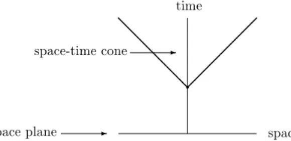
In their paper, the random walk starts at 0 and has transition rates as inFig. 1: on ahole(i.e., on a 0) the random walk has rateαto jump one unit to the left and rateβ to jump one unit to the right, while on a particle(i.e., on a 1) the rates are reversed (w.l.o.g. it may be assumed that 0 < β < α < ∞, so that the random walk has a drift to the left on holes and a drift to the right on particles). Hereafter, we will refer to this model as the(α, β)-model. The LLN is proved under the assumption that the IPS satisfies a space–time mixing property calledcone-mixing(see Fig. 2), which means that the states inside a space–time cone are almost independent of the states in a space plane far below this cone. The proof uses a regeneration scheme originally developed by Comets and Zeitouni [5] for RWRE and adapted to deal with RWDRE. This proof can be easily extended toZd,d ≥2, with the appropriate corresponding notion of cone-mixing.
1.2. Elliptic vs. non-elliptic
The original motivation for the present paper was to study the(α, β)-model in the limit as
Fig. 2. Cone-mixing property: asymptotic independence of states inside a space–time cone from states inside a space plane.
Matic [9], where a recurrence vs. transience criterion, respectively, a large deviation principle are derived.
In the RW(D)RE literature, ellipticity assumptions play an important role. In the static case, RWRE inZd,d≥1, is calledellipticwhen, almost surely w.r.t. the random environment, all the rates arefiniteand there is a basis{ei}1≤i≤d ofZd such that the rate to go fromxtox+ei is
positivefor 1 ≤ i ≤ d. It is calleduniformly ellipticwhen these rates arebounded away from infinity, respectively,bounded away from zero. In [5], in order to take advantage of the mixing property assumed on the random environment, it is important to have uniform ellipticity not necessarily in all directions, but in at least one direction in which the random walk is transient. One way to state this “uniform directional ellipticity” in a way that encompasses also the dynamic setting is to require the existence of a deterministic timeT >0 and a vectore∈Zdsuch that the quenched probability for the random walk to displace itself alongeduring timeT is uniformly positive for almost every realization of the random environment. This is satisfied by the(α, β) -model for e = 0 and any T > 0. This model is also transient (indeed, non-nestling) in the time direction, which enables the use of the cone-mixing property of [2]. In the case of the
(∞,0)-model, however, there are in general no suchT ande. For example, when the random environment is a spin-flip system with bounded flip rates, any fixed space–time position has positive probability of being unreachable by the random walk. For all such models, the approach in [2] fails.
In the present paper, in order to deal with the possible lack of ellipticity we require a different space–time mixing property for the dynamic random environment, which we callconditional cone-mixing. Moreover, as in [5,2], we must require the random walk to have a tendency to stay inside space–time cones. Under these assumptions, we are able to set up a regeneration scheme and prove a LLN. Our result includes the LLN for the(α, β)-model in [2], the(∞,0)-model for at least two subclasses of IPSs that we will exhibit, as well as models that are intermediate, in the sense that they are neither uniformly elliptic in any direction, nor deterministic as the
(∞,0)-model.
1.3. Outline
The rest of the paper is organized as follows. In Section2 we discuss, still informally, the
or have finite range and a small enough ratio of maximal/minimal flip rates. Section5contains preparation material, given in a general context, that is used in the proof of the LLN given in Section6. In Section7we verify our hypotheses for the two classes of IPSs described in Sec-tion4. We also obtain a criterion to determine the sign of the speed in the LLN, via a comparison with independent spin-flip systems. Finally, in Section8, we discuss how to adapt the proofs in Section7to other models, namely, generalizations of the(α, β)-model and the(∞,0)-model, and mixtures thereof. We also give an example where our hypotheses fail. The examples in our paper are all one-dimensional, even though our LLN is valid inZd,d ≥1.
2. Motivation
2.1. The(∞,0)-model
Let
ξ :=(ξt)t≥0 withξt :=ξt(x)x∈Z (2.1)
be a c`adl`ag Markov process onΩ. We will interpretξ by saying that at timet sitex contains either ahole(ξt(x) = 0) or a particle(ξt(x) = 1). Typical examples are interacting particle systems onΩ, such as independent spin-flips and simple exclusion.
Suppose that we run the(α, β)-model onξ with 0< β ≪1≪α <∞. Then the behavior of the random walk is as follows. Suppose that ξ0(0) = 1 and that the walk starts at 0. The walk rapidly moves to the first hole on its right, typically before any of the particles it encounters manages to flip to a hole. When it arrives at the hole, the walk starts to rapidly jump back and forth between the hole and the particle to the left of the hole: we say that it sits in atrap. If
ξ0(0) = 0 instead, then the walk rapidly moves to the first particle on its left, where it starts to rapidly jump back and forth in a trap. In both cases, before moving away from the trap, the walk typically waits until one or both of the sites in the trap flip. If only one site flips, then the walk typically moves in the direction of the flip until it hits a next trap, etc. If both sites flip simultaneously, then the probability for the walk to sit at either of these sites is close to 12, and hence it leaves the trap in a direction that is close to being determined by an independent fair coin.
The limiting dynamics whenα→ ∞andβ ↓0 can be obtained from the above description by removing the words “rapidly, “typically” and “close to”. Except for the extra Bernoulli (12) random variables needed to decide in which direction to go to when both sites in a trap flip simultaneously, the walk up to timet is a deterministic functional of(ξs)0≤s≤t. In particular, if ξ changes only by single-site flips, then apart from the first jump the walk is completely deterministic. Since the walk spends all of its time in traps where it jumps back and forth between a hole and a particle, we may imagine that it lives on the edges ofZ. We implement this observation by associating with each edge its left-most site, i.e., we say that the walk is atx
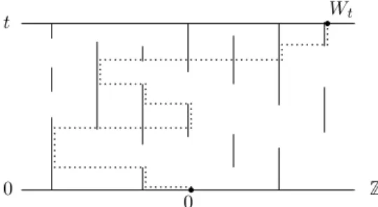
when we actually mean that it is jumping back and forth betweenxandx+1. SeeFig. 3. Let
W :=(Wt)t≥0 (2.2)
denote the random walk path. By the description above,W is c`adl`ag and
Fig. 3. The vertical lines represent the presence of particles. The dotted line is the path of the(∞,0)-walk.
whereYis a sequence of i.i.d. Bernoulli(12) random variables independent ofξ. Note thatWalso has the following three properties:
(1) For any fixed times, the incrementWs+t −Ws is found by applying the same function in (2.3)to the environment shifted in space and time by(Ws,s)and an independent copy ofY; in particular, the pair(Wt, ξt)is Markovian.
(2) Given thatW stays inside a space–time cone until timet,(Ws)0≤s≤t is a functional only of
Y and of the states inξ up to timet inside a slightly larger cone, obtained by adding all neighboring sites to the right.
(3) Each jump of the path follows the same mechanism as the first jump, i.e., Wt −Wt− is computed using the same rules as those for W0but applied to the environment shifted in space and time by(Wt−,t).
The reason for emphasizing these properties will become clearer in Section2.2.
2.2. Regeneration
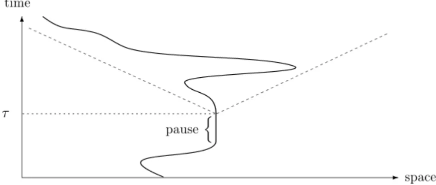
The cone-mixing property that is assumed in [2] to prove the LLN for the(α, β)-model can be loosely described as the requirement that all the states of the IPS inside a space–time cone opening upwards depend weakly on the states inside a space plane far below the tip (recallFig. 2). Let us give a rough idea of how this property can lead toregeneration. Consider the event that the walk stands still for a long time. Since the jump times of the walk are independent of the IPS, so is this event. During this pause, the environment around the walk is allowed to mix, which by the cone-mixing property means that by the end of the pause all the states inside a cone with a tip at the space–time position of the walk are almost independent of the past of the walk. If thereafter the walk stays confined to the cone, then its future increments will be almost independent of its past, and so we get an approximate regeneration. Since in the(α, β)-model there is a uniformly positive probability for the walk to stay inside a space–time cone with a large enough inclination, we see that this regeneration strategy can indeed be made to work. SeeFig. 4.
For the actual proof of the LLN in [2], cone-mixing must be more carefully defined. For technical reasons, there must be some uniformity in the decay of correlations between events in the space–time cone and in the space plane. This uniformity holds, for instance, for any spin-flip system in theM < ϵregime (Liggett [6], Section I.3), but not for the exclusion process or the supercritical contact process. Therefore the approach outlined above works for the first IPS, but not for the other two.
Fig. 4. Regeneration at timeτ.
is important that the pair (IPS, walk) is Markovian and that the law of the environment as seen from the walk at any time is comparable to the initial law. Second, there is a uniformly positive probability for the walk to stand still for a long time and afterwards stay inside a space–time cone. Third, once the walk stays inside a space–time cone, its increments depend on the IPS only through the states inside that cone. Let us compare these observations with what happens in the
(∞,0)-model. Property (1) from Section2.1gives us the Markov property, while property (2) gives us the measurability inside cones. As we will see, when the environment is translation-invariant, property (3) implies absolute continuity of the law of the environment as seen from the walk at any positive time with respect to its counterpart at time zero. Therefore, as long as we can make sure that the walk has a tendency to stay inside space–time cones (which is reasonable when we are looking for a LLN), the main difference is that the event of standing still for a long time is not independent of the environment, but rather is adeterministicfunctional of the environment. Consequently, it is not at all clear whether cone-mixing is enough to allow for regeneration. On the other hand, the event of standing still is local, since it only depends on the states of the two neighboring sites of the trap where the walk is pausing. For many IPSs, the observation of a local event will not affect the weak dependence between states that are far away in space–time. Hence, if such IPSs are cone-mixing, then states inside a space–time cone remain almost independent of the initial configuration even when we condition on seeing a trap for a long time.
Thus, under suitable assumptions, the event “standing still for a long time” is a candidate to induce regeneration. In the(α, β)-model this event does not depend on the environment whereas in the (∞,0)-model it is a deterministic functional of the environment. If we put the(α, β) -model in the form(2.3)by taking forY two independent Poisson processes with ratesαandβ, then we can restate the previous sentence by saying that in the(α, β)-model the regeneration-inducing event depends only onY, while in the(∞,0)-model it depends only onξ. We may therefore imagine that, also for other models of the type(2.3)and that share properties (1)–(3), it will be possible to find more general regeneration-inducing events that depend on bothξ and
Y in a non-trivial manner. This motivates our setup in Section3.
3. Model setting
environment ξ. Notation is set up in Section 3.1. Section 3.2 contains the three structural assumptions that define the class of models we will consider.
3.1. Notation and setup
LetN= {1,2, . . .}be the set of natural numbers, andN0:=N∪ {0}. LetEbe a Polish space andξ :=(ξt)t≥0a Markov process with state spaceEZd whered ∈N. LetY :=(Yn)n∈Nbe an i.i.d. sequence of random elements independent ofξ. ForI ⊂ [0,∞), abbreviateξI :=(ξu)u∈I, and analogously forY. The joint law ofξ andY whenξ0=η∈EZ
d
will be denoted byPη. For
n∈N, putYn:=σ(Y[1,n]). LetF0:=σ (ξ0)and, fort>0,Ft :=σ(ξ[0,t])∨Y⌈t⌉. Fort ≥0 andx∈Zd, letθtandθx be the time-shift and space-shift operators given by
θt(ξ,Y):=(ξt+s)s≥0, (Y⌊t⌋+n)n∈N, θx(ξ,Y):=(θxξt)t≥0, (Yn)n∈N, (3.1)
whereθxξt(y)=ξt(x+y). In the sequel, whetherθis a time-shift or a space-shift operator will always be clear from the index.
We assume thatξ is translation-invariant, i.e.,θxξ has underPη the same distribution as ξ under Pθxη. We also assume the existence of a (not necessarily unique) translation-invariant equilibrium distributionµ forξ, and write Pµ(·) := µ(dη)Pη(·)to denote the joint law of
ξandY whenξ0is drawn fromµ.
The random walk will be denoted byW =(Wt)t≥0, and we will writeξ¯:=(ξ¯t)t≥0to denote theenvironment process as seen from W, i.e.,ξ¯t :=θWtξt. Letµ¯t denote the law ofξ¯tunderPµ.
We abbreviateµ¯ := ¯µ0. Note thatµ¯ =µwhenPµ(W0=0)=1. Form>0 andR∈N0, define theR-enlargedm-cone by
CR(m):=
(x,t)∈Zd× [0,∞): ∥x∥ ≤mt+R, (3.2)
where∥ · ∥is theL1norm. LetCR,t(m)be theσ-algebras generated by the states ofξup to time
tinsideCR(m).
3.2. Structural assumptions
We will assume thatW is random translation of a random walk starting at 0. More precisely, we assume thatZ =(Zt)t≥0is a c`adl`agF-adaptedZd-valued process withZ0=0Pµ¯-a.s. such that
Wt =W0+θW0Zt ∀t≥0. (3.3)
We also assume thatW0∈Zdand depends onξ andY only throughξ0, i.e.,
Pµ(W0=x |F∞)=Pµ(W0=x|ξ0) a.s.∀x∈Zd. (3.4) Under these assumptions,(Wt −W0)t≥0has underPµthe same distribution as Z underPµ¯. In what follows we makethree structural assumptionsonZ:
(A1) (Additivity)
For alln∈N,
(Zt+n−Zn)t≥0=θZnθnZ Pµ¯-a.s. (3.5)
(A2) (Locality)
(A3) (Homogeneity of jumps)
For alln∈Nandx∈Zd, Pµ¯
Zn−Zn−=x |ξ[0,n],Z[0,n)
=Pθ
Zn−ξn
W0=x
Pµ¯-a.s. (3.6)
These properties are analogs of properties (1)–(3) of the(∞,0)-model mentioned in Section2.1, with the difference that we only require them to hold at integer times; this will be enough as our proof relies on integer-valued regeneration times. We also assume the ‘extra randomness’
Y to be split independently among time intervals of length 1; for example, in the case of the
(∞,0)-model, each Yn wouldnotbe a Bernoulli(12) random variable but a wholesequenceof such variables instead. This is discussed in detail in Section7.1.
Another remark: assumption (A3) might seem strange since many random walk models have no deterministic jumps, which is indeed the case for the examples described in Section4. Note however that, in this case, (A3) severely restrictsW0, implyingW0=0 a.s. whenξis started from
θZn−ξn. Furthermore, our main theorem (Theorem 4.1below) is not restricted to this situation and
includes also cases with deterministic jumps. For example, one could modify the(∞,0)-walk to jump exactly at integer times. Additional examples with deterministic jumps are described in item 4 of Section8. The relevance of assumption (A3) is in showing that the law of the environment as seen by the RW after any jump is absolutely continuous w.r.t. the law after the first jump; this is done inLemma 6.1below.
4. Main results
Theorems 4.1and4.2below are the main results of our paper.Theorem 4.1in Section4.1is our LLN.Theorem 4.2in Section4.2verifies the hypotheses in this LLN for the(∞,0)-model in two classes of one-dimensional IPSs. For these classes some more information is available, namely, convergence inLp, p≥1, and a criterion to determine the sign of the speed.
4.1. Law of large numbers
In order to develop a regeneration scheme for a random walk subject to assumptions (A1)–(A3) based on the heuristics discussed in Section 2.2, we need suitable regeneration-inducing events. In thefour hypothesesstated below, these events appear as a sequence(ΓL)L∈N such that, for a certain fixedm∈(0,∞)andRas in (A2),ΓL ∈CR,L(m)∨YLfor allL ∈N.
(H1) (Determinacy)
OnΓL,Zt =0 for allt ∈ [0,L]Pµ¯-a.s.
(H2) (Non-degeneracy)
ForL large enough, there exists aγL >0 such thatPη(ΓL)≥γL forµ¯-a.e.η.
(H3) (Cone constraints)
Let S := inf{t > 0: ∥Zt∥ > mt}. Then there exist a ∈ (1,∞), κL ∈ (0,1] and
ψL ∈ [0,∞)such that, forL large enough andµ¯-a.e.η,
(1) Pη(θLS = ∞ |ΓL)≥κL,
(2) Eη
1{θLS<∞}(θLS) a|Γ
L≤ψLa.
(4.1)
(H4) (Conditional cone-mixing)
There exists a sequence of non-negative numbers(ΦL)L∈Nsatisfying limL→∞κL−1ΦL =0 such that, forLlarge enough and forµ¯-a.e.η,
Eη(θLf |ΓL)−Eµ¯(θLf |ΓL)
We are now ready to state our LLN.
Theorem 4.1. Under assumptions(A1)–(A3)and hypotheses(H1)–(H4), there exists aw∈Rd
such that
lim t→∞t
−1W
t =w Pµ−a.s. (4.3)
Remark 1. Hypothesis (H4) above without the conditioning onΓL in(4.2)and with constantκL is the same as the cone-mixing condition used by Avena et al. [2]. There,W0=0Pµ-a.s., so that
¯
µ=µ.
Remark 2. Theorem 4.1provides no information about the value ofw, not even its sign when
d=1. Understanding the dependence ofwon model parameters is in general a highly non-trivial problem.
4.2. Examples
We next describe two classes of one-dimensional IPSs for which the(∞,0)-model satisfies hypotheses (H1)–(H4). Further details will be given in Section7. In both classes,ξ is a spin-flip system inΩ= {0,1}Zwith bounded and translation-invariant single-site flip rates. We may assume that the flip rates at the origin are of the form
c(η)=
c0+λ0p0(η) ifη(0)=1,
c1+λ1p1(η) ifη(0)=0, η
∈Ω, (4.4)
for someci, λi ≥0 andpi: Ω→ [0,1],i =0,1.
Example 1. c(·)is in theM < ϵregime (see Liggett [6], Section I.3).
Example 2. p(·)has finite range and(λ0+λ1)/(c0+c1) < λc, whereλcis the critical infection rate of the one-dimensional contact process with the same range.
Theorem 4.2. Consider the(∞,0)-model. Suppose that ξ is a spin-flip system with flip rates given by(4.4). Then forExamples1and2there exist a version of ξ and eventsΓL ∈CR,L(m)∨ YL, L ∈ N, satisfying hypotheses (H1)–(H4). Furthermore, the convergence inTheorem4.1
holds also in Lpfor all p≥1, and
w≥ c0+λ0
c1+c0+λ0
(c1−c0−λ0) if c1≥c0+λ0,
w≤ − c1+λ1
c0+c1+λ1(
c0−c1−λ1) if c0≥c1+λ1.
(4.5)
For independent spin-flip systems (i.e., whenλ0 = λ1 =0),(4.5)shows thatwis positive, zero or negative when the densityc1/(c0+c1)is, respectively, larger than, equal to or smaller than12. The criterion for otherξ is obtained by comparison with independent spin-flip systems.
Additional models will be discussed in Section 8. We will consider generalizations of the
(α, β)-model and the(∞,0)-model, namely,internal noisemodels andpatternmodels, as well
as mixtures of them. The verification of (H1)–(H4) will be analogous to the two examples discussed above and will not be carried out in detail.
This concludes the motivation and the statement of our main results. The remainder of the paper will be devoted to the proofs ofTheorems 4.1and4.2, with the exception of Section8, which contains additional examples and remarks.
5. Preparation
The aim of this section is to prove two propositions (Propositions 5.2and5.4below) that will be needed in Section6to prove the LLN. In Section5.1we deal with approximate laws of large numbers for general discrete- or continuous-time random walks inRd. In Section5.2we specialize to additive functionals of a Markov chain whose transition kernel satisfies a certain absolute-continuity property.
5.1. Approximate law of large numbers
This section contains two fundamental facts that are the basis of our proof of the LLN. They deal with the notion of an approximate law of large numbers.
Definition 5.1. LetW =(Wt)t≥0be a random process inRd witht ∈ N0ort ∈ [0,∞). For
ε ≥ 0 and v ∈ Rd, we say that W has anε-approximate asymptotic velocityv, written as
W ∈ AV(ε, v), if
lim sup t→∞
Wt
t −v
≤ε a.s. (5.1)
We take∥ · ∥to be theL1-norm. A simple observation is thatW a.s. has an asymptotic velocity if and only if for everyε > 0 there exists avε ∈ Rd such that W ∈ AV(ε, vε). In this case limε↓0vεexists and is equal to the asymptotic velocity.
5.1.1. First key proposition: skeleton approximate velocity
The following proposition gives conditions under which an approximate velocity for the process observed along a random sequence of times implies an approximate velocity for the full process.
Proposition 5.2. Let W be as in Definition 5.1. Set τ0 := 0, let (τk)k∈N be an increasing
sequence of random times in(0,∞)(orN) withlimk→∞τk = ∞a.s. and put Xk :=(Wτk, τk)∈ Rd+1, k∈N0. Suppose that the following hold:
(i) There exists an m>0such that
lim sup k→∞
sup s∈(τk,τk+1]
Ws−Wτk
s−τk
≤m a.s. (5.2)
Proof. First, let us check that (i) implies
lim sup t→∞
∥Wt∥
t ≤m a.s. (5.3)
Suppose that
lim sup k→∞
sup s>τk
Ws−Wτk
s−τk
≤m a.s. (5.4)
Since, for everykandt > τk, Wt t
≤ ∥Wτk∥
t +
Wt−Wτk
t−τk
1−
τk
t
≤
∥Wτk∥
t +ssup>τk
Ws−Wτk
s−τk
1−
τk
t
, (5.5)
(5.3)follows from(5.4)by lettingt → ∞followed byk→ ∞. To check(5.4), define, fork∈N0andl∈N,
m(k,l):= sup s∈(τk,τk+l]
Ws−Wτk
s−τk
and
m(k,∞):= sup s>τk
Ws−Wτk
s−τk
= lim
l→∞m(k,l). (5.6)
Using the fact that(x1+x2)/(y1+y2)≤(x1/y1)∨(x2/y2)for allx1,x2∈ Randy1,y2>0, we can prove by induction that
m(k,l)≤max{m(k,1), . . . ,m(k+l−1,1)}, l∈N. (5.7)
Fixε >0. By (i), a.s. there exists akεsuch thatm(k,1)≤m+εfork>kε. By(5.7), the same is true form(k,l)for alll∈N, and therefore also form(k,∞). Sinceεis arbitrary,(5.4)follows.
Let us now proceed with the proof of the proposition. Assumption (ii) implies that, a.s.,
lim sup k→∞
Wτk k −v
≤ε and lim sup k→∞
τk
k −u
≤ε. (5.8)
Fort ≥0, letktbe the (random) non-negative integer such that
τkt ≤t< τkt+1. (5.9)
Sinceτ1<∞a.s.,kt >0 for large enought. From(5.8)and(5.9)we deduce that
lim sup t→∞ t kt −u
≤ε and so lim sup t→∞ t kt
−τkt
kt
≤2ε. (5.10)
Fortlarge enough we may write
uWt
t −v
≤ ∥Wt∥
t
u− t
kt +
Wt−Wτkt
kt +
Wτkt kt −v
≤ ∥Wt∥
t
u− t
kt + sup s∈(τkt,τkt+1]
Ws−Wτkt
s−τk
t
t−τk
t kt +
Wτkt kt −v , (5.11)
5.1.2. Conditions for the skeleton to have an approximate velocity
The following lemma states sufficient conditions for a discrete-time process to have an approximate velocity. It will be used in the proof ofProposition 5.4below.
Lemma 5.3. Let X =(Xk)k∈N0 be a sequence of random vectors inR
dwith joint law P such
that P(X0 = 0) = 1. Suppose that there exist a probability measure Q onRd and numbers
φ∈ [0,1), a>1, K >0with
Rd∥x∥
aQ(d x)≤Ka, such that, P-a.s. for all k∈ N0, (i) |P(Xk+1−Xk∈ A| X0, . . . ,Xk)−Q(A)| ≤φfor all A measurable;
(ii) E[∥Xk+1−Xk∥a|X0, . . . ,Xk] ≤Ka. Then
lim sup n→∞ Xn
n −v
≤2Kφ(a−1)/a P-a.s., (5.12)
wherev=
Rdx Q(d x). In other words, X∈ AV(2Kφ
(a−1)/a, v).
Proof. The proof is an adaptation of the proof of Lemma 3.13 in [5]; we include it here for
completeness. With regular conditional probabilities, we can, using (i), couple P and Q⊗N0
according to a standard splitting representation (see e.g. Berbee [4]). More precisely, on an enlarged probability space we can construct random variables
(∆k,Vk,Rk)k∈N (5.13)
such that
(1) (∆k)k∈Nis an i.i.d. sequence of Bernoulli(φ) random variables. (2) (Vk)k∈Nis an i.i.d. sequence of random vectors with lawQ. (3) (∆l)l≥kis independent of(∆l,Vl,Rl)0≤l<k,Rk.
(4) SettingXˆ0 :=0 and, fork ∈ N0,Xˆk+1− ˆXk :=(1−∆k)Vk +∆kRk, then Xˆ is equal in distribution toX.
(5) SettingGk :=σ (∆l,Vl,Rl: 0 ≤ l ≤ k), thenE[f(Vk)| Gk−1]is measurable w.r.t.σ (Xˆl: 0≤l ≤k−1)for any Borel nonnegative function f.
Using (4), we may write
Xn n d = ˆ Xn n = 1 n n k=1
Vk− 1
n
n
k=1
∆kVk+ 1
n
n
k=1
∆kRk. (5.14)
Asn → ∞, the first term on the r.h.s. converges a.s. tovby the LLN for i.i.d. random variables. By H¨older’s inequality, the norm of the second term is at most
1 n n k=1 ∆k
(a−1)/a 1
n
n
k=1
∥Vk∥a 1/a
, (5.15)
which, by (1) and (2), converges a.s. asn→ ∞to
φ(a−1)/a
Rd
∥x∥aQ(d x)
1/a
≤ Kφ(a−1)/a. (5.16)
To control the third term, putRk∗:=E[Rk |Gk−1]. Since∥∆kRk∥ ≤ ∥ ˆXk+1− ˆXk∥, using (1), (3), (4), (5) and (ii), we get
Combining(5.17)with Jensen’s inequality, we obtain
∥Rk∗∥ ≤E∥Rk∥a|Gk−11/a≤
K
φ1/a, (5.18)
so that 1 n n k=1
∆kRk∗ ≤ K
φ1/a 1 n n k=1 ∆k −−−→
n→∞ Kφ
(a−1)/a. (5.19)
Now fixy∈Rdand put
Mny := n
k=1
∆k
k ⟨Rk−R
∗
k,y⟩ (5.20)
where⟨·,·⟩denotes the usual inner product. Then(Mny)n∈N0 is a (Gn)n∈N0-martingale whose quadratic variation is
⟨My⟩n=
n
k=1
∆k
k2⟨Rk−R ∗
k,y⟩2. (5.21)
By the Burkholder–Gundy inequality and(5.17)–(5.18), we have
E
sup n∈N
|Mny|a∧2
≤C E⟨My⟩(∞a∧2)/2
≤C E
∞
k=1
∆k
ka∧2
⟨Rk−Rk∗,y⟩
a∧2
≤C∥y∥a∧2Ka∧2, (5.22)
whereC is a positive constant that may change after each inequality. This implies that Mny is uniformly integrable and therefore converges a.s. asn→ ∞. Kronecker’s lemma then gives
lim n→∞ 1 n n k=1
∆k⟨Rk−R∗k,y⟩ =0 a.s. (5.23)
Sinceyis arbitrary, this in turn implies that
lim n→∞ 1 n n k=1
∆k(Rk−R∗k)=0 a.s. (5.24)
Therefore, by(5.19)and(5.24), the limsup of the norm of the last term in the r.h.s. of(5.14)is also bounded byKφ(a−1)/a, which finishes the proof.
5.2. Additive functionals of a discrete-time Markov chain 5.2.1. Notation
LetX = (Xn)n∈N0 be a time-homogeneous Markov chain in the canonical space equipped
with the time-shift operators(θn)n∈N0. Forn≥1, putFn :=σ(X[1,n])(note thatX0̸∈F∞) and
letPχ denote the law of(Xn)n∈N0 whenX0=χ. Fix an initial measureνand suppose that, for
any nonnegative f ∈F∞,
Pν(EXn[f] ∈ ·)≪Pν(EX0[f] ∈ ·), (5.25)
Let Z =(Zn)n∈N0 be a Z
d-valued F-adapted process that is an additive functional of
(Xn)n∈N, i.e.,Z0=0 and, for anyk∈N0,
(Zk+n−Zk)n∈N0 =θkZ Pν-a.s. (5.26)
We are interested in finding random times(τk)k∈N0 such that(Zτk, τk)k∈N0 satisfies the
hy-potheses ofLemma 5.3. In the Markovian setting it makes sense to look forτkof the form
τ0=0, τk+1=τk+θτkτ, k∈N0, (5.27)
whereτ is a random time.
Condition (i) ofLemma 5.3is a “decoupling condition”. It states that the law of an increment of the process depends weakly on the previous increments. Such a condition can be enforced by the occurrence of a “decoupling event” under which the increments of(Zτk, τk)k∈N0 lose dependence. In this setting,τ is a time at which the decoupling event is observed.
5.2.2. Second key proposition: approximate regeneration times
Proposition 5.4below is a consequence ofLemma 5.3and is the main result of this section. It will be used together withProposition 5.2to prove the LLN in Section6. It gives a way to constructτ when the decoupling event can be detected by “probing the future” with a stopping time.
For a random variableT taking values inN0∪ {∞}, we define theimageofT byIT := {n∈ N: Pν(T =n) >0}, and its closure under addition byI¯T := {n ∈ N: ∃l ∈N,i1, . . . ,il ∈ IT : n =i1+ · · · +il}. Note thatIT = ∅if and only ifT ∈ {0,∞}a.s.
Proposition 5.4. LetT be a stopping time for the filtrationF taking values in N∪ {∞}. Put
D:= {T = ∞}and suppose that the following properties hold:
(i) For every n∈ ¯IT there exists a Dn∈Fnsuch that
D∩θnD=Dn∩θnD Pν-a.s.
(ii) There exist numbersρ∈(0,1], a>1, C >0, m>0andφ∈ [0,1)such that, Pν-a.s.,
(a) PX0(D)≥ρ,
(b) EX0
1{T<∞}Ta≤Ca, (c) On D,∥Zt∥ ≤mt for all t∈N0, (d)
EX0
f(Z, (θnT)n∈ ¯IT)| D
−Eνf(Z, (θnT)n∈ ¯IT)| D
≤φ∥f∥∞ ∀f ≥ 0
mea-surable.
Then there exists a random timeτ ∈F∞taking values inNsuch that, settingτk as in(5.27)
and Xk :=(Zτk, τk), then X ∈ AV(ε, (v,u))where(v,u)= Eν[(Zτ, τ)| D], u >0and
ε=12(m+1)uφ(a−1)/a.
5.2.3. Two further propositions
In order to proveProposition 5.4, we will need two further propositions (Propositions 5.5and 5.6below).
Proposition 5.5. Letτ be a random time measurable w.r.t.F∞taking values in N. Put τk as
in(5.27)and Xk :=(Zτk, τk). Suppose that there exists an event D∈F∞such that the following
(i) For n∈Iτ, there exist events Hnand Dn∈Fnsuch that
(a) {τ =n} = Hn∩θnD,
(b) D∩θnD=Dn∩θnD.
(5.28)
(ii) There existφ∈ [0,1), K >0and a>1such that, on{PX0(D) >0},
(a) EX0[∥X1∥
a|D] ≤Ka,
(b) PX0(X1∈ A|D)−Pν(X1∈ A|D)
≤φ ∀A measurable.
(5.29)
Then X ∈ AVε, (v,u), whereε=2Kφ(a−1)/aand(v,u):=Eν[X1|D].
Proof. Sinceτ < ∞, by (i)(a) and(5.25)we must have Pν(D) >0. LetFτk be theσ-algebra of the events B ∈ F∞such that, for alln ∈ N, there exists Bn ∈ Fn with B∩ {τk = n} =
Bn∩ {τk =n}. We will show that,Pν-a.s., for allk∈N,
Eν∥θτ
kX1∥ a|F
τk
≤Ka (5.30)
and Pν
θ
τkX1∈ A|Fτk
−
Pν(X1∈ A|D)
≤φ ∀Ameasurable. (5.31)
Then, settingQ(·):= Pν(X1∈ ·|D)and noting thatθτkX1 =Xk+1−XkandXj ∈Fτk for all
0≤ j ≤k, we will be able to conclude since(5.30)–(5.31)and (ii)(a) imply that the conditions ofLemma 5.3are all satisfied.
To prove(5.30)–(5.31), first note that, using (i), one can verify by induction that (i)(a) holds also forτk, i.e., for everyn ∈Iτk there existsHk,n∈Fnsuch that
{τk=n} = Hk,n∩θnD Pν-a.s. (5.32)
TakeB∈Fτkand a measurable nonnegative function f, and write
Eν
1Bθτkf(X1)
= n∈Iτk
Eν
1B∩{τk=n}θnf(X1)
= n∈Iτk
Eν
1Bn∩Hk,nθn
1Df(X1)
=
n∈Iτk
Eν
1Bn∩Hk,nPXn(D)EXn[f(X1)|D]
.
(5.33)
Noting that Pν(B)= n∈Iτk Eν
1Bn∩Hk,nPXn(D)
, obtain(5.30)by taking f(x)= ∥x∥aand using (ii)(a) together with(5.25). For(5.31), choose f =1A, subtract Pν(B)Eν[f(X1)|D] from (5.33)and use (ii)(b).
Proposition 5.6.Let T be a stopping time as in Proposition5.4and suppose that conditions
(ii)(a)and(ii)(b)of that proposition are satisfied. Define a sequence of stopping times(Tk)k∈N0
as follows. Put T0=0and, for k∈N0,
Tk+1:= ∞
if Tk= ∞
Tk+θTkT otherwise.
(5.34)
Put
N:=inf{k∈N0: Tk <∞and Tk+1= ∞}. (5.35)
Then N<∞a.s. and there exists a constant~=~(a, ρ)∈(0,∞)such that, Pν-a.s., EX0
TNa≤(~
C)a. (5.36)
Proof. First, let us check that
PX0(N ≥n)≤(1−ρ)
n. (5.37)
Indeed,N ≥nif and only ifTn<∞, so that, fork∈N0,
PX0(Tk+1<∞)=EX0
1{Tk<∞}PXTk(T <∞)
≤(1−ρ)PX0(Tk<∞), (5.38)
where we use (ii)(a) and the fact that(5.25)holds also with a stopping time in place ofn. Clearly, (5.37)follows from(5.38)by induction. In particular,N<∞a.s.
From(5.34)we see that, for 0≤k≤n,
Tn=Tk+θTkTn−kon{Tk <∞}. (5.39)
Using (ii)(a) and (b), with the help of(5.25)again, we can a.s. estimate, for 0≤k<n,
EX0
1{Tn<∞}|Tk+1−Tk| a
= EX0
1{Tk+1<∞}|Tk+1−Tk| aP
XTk+1(Tn−k−1<∞)
≤ (1−ρ)n−k−1EX0
1{Tk<∞,θTkT<∞}θTkT a
=(1−ρ)n−k−1EX0
1{Tk<∞}EXTk
1{T<∞}Ta
≤ (1−ρ)n−k−1CaPX0(Tk <∞)
≤ (1−ρ)n−1Ca. (5.40)
Now write
TN = N−1
k=0
Tk+1−Tk. (5.41)
By Jensen’s inequality,
TNa ≤Na−1
N−1
k=0
|Tk+1−Tk|a (5.42)
so that, by(5.40),
EX0
TNa≤
∞
n=1
na−1
n−1
k=0
EX0
1{N=n}|Tk+1−Tk|a≤Ca ∞
n=1
na(1−ρ)n−1 a.s. (5.43)
and(5.36)follows by taking~=∞
n=1na(1−ρ)n−1 1/a
.
As for the claim thatITN ⊂ ¯IT, write, forn∈N,
{TN =n} = ∞
k=1
{Tk =n,N =k} (5.44)
to see thatITN ⊂
∞
5.2.4. Proof ofProposition 5.4
We can now combinePropositions 5.5and5.6to proveProposition 5.4.
Proof. In the following we will refer to the hypotheses ofProposition 5.5with the prefix P. For example, P(i)(a) denotes hypothesis (i)(a) in that proposition. The hypotheses inProposition 5.4 will be referred to without a prefix. Since the hypotheses ofProposition 5.6are a subset of those ofProposition 5.4, the conclusions of the former are valid.
We will show that, ifτ :=t0+θt0TN for a suitablet0∈N, thenτ satisfies the hypotheses of
Proposition 5.5for a suitableK. There are two cases. IfIT = ∅, thenTN≡0. Choosingt0=1, we basically fall in the context ofLemma 5.3. P(i)(a) and P(i)(b) are trivial, (ii)(c) implies that P(ii)(a) holds withK =(m+1), while P(ii)(b) follows immediately from (ii)(d). Therefore, we may suppose thatIT ̸= ∅and putι:=minIT ∈N. LetCˆ :=1∨(~C)andt0:=ι⌈ ˆCρ−1/a⌉. We will show thatτ satisfies the hypotheses ofProposition 5.5withK =6ι(m+1)Cˆρ−1/a. P(i)(a): First we show that this property is true forTN. Indeed,
{TN =n} =
k∈N0
{N =k,Tk=n} =
k∈N0
{Tk=n, θnT = ∞} (5.45)
=θnD∩
k∈N0
{Tk =n}
, (5.46)
andHˆn := k∈N0{Tk = n} ∈ Fn since theTk’s are all stopping times. Now we observe that
{τ =n} =θt
0{TN =n−t0}, so we can takeHn:= ∅ifn<t0andHn:=θt0Hˆn−t0otherwise.
P(i)(b): By (i), it suffices to show thatIτ ⊂ ¯IT. Sincet0∈ ¯IT (as an integer multiple ofι), this
follows from the definition ofτ and the last conclusion ofProposition 5.6.
P(ii)(a): By (ii)(c),∥X1∥a=(∥Zτ∥ +τ)a≤((m+1)τ)aonD. Therefore, we just need to show that
EX0
τa|D
≤(6ιCˆ)a/ρ. (5.47)
Now,τa≤2a−1
t0a+θt
0T a N
and, byProposition 5.6and(5.25),
EX0
θt0T a N
=EX0
EXt0
TNa≤ ˆCa. (5.48)
Using (ii)(a), we obtain
EX0
θ t0T
a N|D
≤ ˆ
Ca/ρ. (5.49)
Sincet0≤2ιCˆρ−1/aandι≥1,(5.47)follows.
P(ii)(b): LetS=(Sn)n∈ ¯IT withSn:=θnT. By (ii)(d), it is enough to show thatX1=(Zτ, τ)∈ σ (Z,S)a.s. SinceZτ =∞
n=01{τ=n}Zn∈σ (Z, τ), it suffices to show thatτ ∈σ(S)a.s. Using the definition of theTk’s, we verify by induction that eachTk is a.s. measurable inσ (S). Since
With all hypotheses verified,Proposition 5.5implies thatX ∈ AV(ε, (v,ˆ u)), where(v,u)=
Eν[X1|D]andεˆ =2Kφ(a−1)/a. To conclude, observe thatu =Eν[τ|D] ≥t0≥ιCˆρ−1/a>0, so thatK =6(m+1)ιCˆρ−1/a ≤ 6(m+1)u. Therefore,εˆ ≤εand the proposition follows. In the caseIT = ∅, we conclude similarly sinceu =1 andK =(m+1).
6. Proof ofTheorem 4.1
In this section we show how to put the model defined in Section3in the context of Section5, and we prove the LLN usingPropositions 5.2and5.4.
6.1. Two further lemmas
Before we start, we first derive two lemmas (Lemmas 6.1and6.2below) that will be needed in Section6.2. The first lemma relates the laws of the environment as seen fromWn and from
W0. The second lemma is an extension of the conditional cone-mixing property for functions that depend also onY.
Lemma 6.1. µ¯n≪ ¯µfor all n∈N.
Proof. Fort ≥0, letµ¯t−denote the law ofθWt−ξt underPµ. First we will show thatµ¯t−≪µ.
This is a consequence of the fact that µis translation-invariant equilibrium, and remains true if we replace Wt− by any random variable taking values in Zd. Indeed, ifµ(A) = 0 then Pµ(θxξt ∈ A)=0 for everyx ∈Zd, so
¯
µt−(A)=Pµ(θWt−ξt ∈ A)=
x∈Zd
Pµ(Wt−=x, θxξt ∈ A)=0. (6.1)
Now taken∈Nand letgn:= d ¯
µn−
dµ . For any measurable f ≥0, Eµf(θWnξn)
=Eµ¯f(θZnξn)
=
x∈Zd Eµ¯
1{Zn−Zn−=x}f(θxθZn−ξn)
=
x∈Zd Eµ¯
PθZn−ξn(W0=x)f(θxθZn−ξn)
=
x∈Zd Eµ
PθWn−ξn(W0=x)f(θxθWn−ξn)
=
x∈Zd
Eµgn(ξ0)Pξ0(W0=x)f(θxξ0)
=
x∈Zd
Eµgn(ξ0)1{W0=x}f(θxξ0)
=Eµgn(ξ0)f(θW0ξ0)
(6.2)
where, for the second equality, we use (A3).
Lemma 6.2. For L large enough and for all nonnegative f ∈CR,∞(m)∨Y∞,
Eη[θLf |ΓL]−Eµ¯[θLf |ΓL]
Proof. Put fy(η) = f(η,y)and abbreviateY(L) =(Yk)k>L. ThenθLf = θLfY(L). SinceΓL depends onY only through(Yk)k≤L, we have
Eη[θLf 1ΓL |Y
(L)] =
EηθLf(·)1ΓL
◦(Y(L)), (6.4)
and(6.3)follows from (H4) applied to fy.
6.2. Proof ofTheorem 4.1
Proof. Extendξ andZ for timest ∈ [−1,0]by taking them constant in this interval, and letY0 be a copy ofY1independent ofF∞. Put
X0:=ξ[−1,0],Z[−1,0],Y0,
Xn+1:=θZnξ[n,n+1], (Zt+n−Zn)0≤t≤1,Yn+1
, n ∈N0. (6.5)
Then(Xn)n∈N0 is a time-homogeneous Markov chain; to avoid confusion, we will denote its
time-shift operator byθ¯n. Note thatFn =Fn∀n ∈ N∪ {∞}and that, for functions f ∈ F∞,
¯
θnf =θZnθnf ∀n ∈N0.
FixL ∈Nlarge enough and put
TL :=L+1ΓL⌈θLS⌉. (6.6)
By(3.5)and sinceΓL ∈FL andZ isF-adapted,TL is anF-stopping time and(Zn)n∈N0 is an
additive functional of(Xn)n∈Nas in Section5.2.
Next, we will verify(5.25)forXand the hypotheses ofProposition 5.4forZandTLunderPµ¯. These hypotheses will be referred to with the prefix P. The notation here is consistent in the sense that parameters in Section3are named according to their role in Section5; the presence/absence of a subscriptLindicates whether the parameter depends onL or not.
(5.25): Noting that, for nonnegative f ∈F∞andn ∈N0,
EXn[f]=EθZnξn[f] Pµ¯-a.s., (6.7)
this follows fromLemma 6.1and(3.3)–(3.4).
P(i): We will findDnforn≥L. This is enough, since bothITLand
¯
ITLare subsets of[L,∞)∩N.
Using (A1) and (H1), we may write
D=ΓL∩ {∥Zt+L∥ ≤mt∀t ≥0},
¯
θnD= ¯θnΓL∩ {∥Zt+n+L−Zn∥ ≤mt ∀t ≥0}.
(6.8)
Intersecting the two above events, we get
D∩ ¯θnD=ΓL∩ {∥Zt∥ ≤mt∀t ∈ [0,n]} ∩ ¯θnD, (6.9) i.e., P(i) holds withDn:=ΓL∩ {∥Zt∥ ≤mt∀t∈ [0,n]} ∈Fnforn≥L.
For the remaining items, note that, by(6.7), the distribution of(Z,TL)underPX0 isPµ¯-a.s.
the same as underPξ0.
P(ii)(a): Since{TL = ∞} = {θLS = ∞} ∩ΓL, we get from (H2) and (H3)(1) that,Pµ¯-a.s.,
Pξ0(TL = ∞)=Pξ0(θLS = ∞ |ΓL)Pξ0(ΓL)≥κLγL >0, (6.10)
P(ii)(b): By the definition ofTL, we have
TLa1{TL<∞} = L a1
Γc
L +(L+ ⌈θLS⌉) a1
ΓL∩{θLS<∞}
≤ La1Γc
L +(L+1+θLS) a1
ΓL∩{θLS<∞}
≤ 2a−1(L+1)a+2a−1(θLS)a1{θLS<∞}
1ΓL. (6.11)
Therefore, by (H3)(2), we get
Eξ0
TLa1{TL<∞}
≤2a((L+1)a+(1∨ψL)a)≤[2(L+1+1∨ψL)]a Pµ¯-a.s., (6.12)
so that we can takeCL :=2(L+1+1∨ψL).
P(ii)(c): This follows from (H1) and the definition ofS.
P(ii)(d): First note that, for anyn ∈ ¯ITL,
¯
θnTL ∈ σ (Z,θ¯nΓL). Sincen ≥ L, on{TL = ∞} = ΓL ∩ {θLS = ∞}, Z, θ¯nΓL and{θLS = ∞} are all measurable in θL(CR,∞(m)∨Y∞); this follows from (A2), (H1) and the assumptions onΓL. Noting that, for any two probability measuresν1,ν2and an eventA,
∥ν1(· | A)−ν2(· |A)∥T V ≤2 ∥ν1−ν2∥T V
ν1(A)∨ν2(A)
(6.13)
where∥ · ∥T V stands for total variation distance, we see that P(ii)(d) follows fromLemma 6.2 and (H3)(1) withφL :=2ΦL/κL →0 asL → ∞by (H4).
Thus, for large enoughL, we can conclude byProposition 5.4that there exists a sequence of times(τk)k∈N0 with limk→∞τk= ∞a.s. such that(Zτk, τk)k∈N0 ∈ AV(εL, (vL,uL)), where
vL =Eµ¯[Zτ1|D],
uL =Eµ¯[τ1|D]>0,
εL =12(m+1)uLφ(La−1)/a.
(6.14)
From(6.14)and P(ii)(c),Proposition 5.2implies thatZ ∈ AV(δL, wL), where
wL =vL/uL,
δL =(3m+1)12(m+1)φ(La−1)/a.
(6.15)
By (H4), limL→∞δL = 0. As was observed after Definition 5.1, this implies that w := limL→∞wL exists and that limt→∞t−1Zt =wPµ¯-a.s., which, by(3.3)–(3.4), implies the same forW,Pµ-a.s.
We have at this point finished the proof of our LLN. In the following sections, we will look at examples that satisfy (H1)–(H4). Section7is devoted to the(∞,0)-model for two classes of one-dimensional spin-flip systems. In Section8we discuss three additional models where the hypotheses are satisfied, and one where they are not.
7. Proof ofTheorem 4.2
We begin with a proper definition of the(∞,0)-model in Section7.1, where we identify Z
(H2) for which we then verify (H3). We also derive uniform integrability properties oft−1Wt which are the key for convergence inLp once we have the LLN. In Sections7.3and7.4, we specialize to particular constructions in order to prove (H4), which is the hardest of the four hypotheses. Section7.5is devoted to proving a criterion for positive or negative speed.
7.1. Definition of the model
Assume thatξ is a c`adl`ag process with state spaceE := {0,1}Z. We will define the walkW in several steps, and a monotonicity property will follow.
7.1.1. Identification of Z and W0
First, letT r+ =T r+(η)andT r−=T r−(η)denote the locations of the closest traps to the right and to the left of the origin in the configurationη∈E, i.e.,
T r+(η):=inf{x∈N0: η(x)=1, η(x+1)=0},
T r−(η):=sup{x∈ −N0: η(x)=1, η(x+1)=0}, (7.1)
with the convention that inf∅ = ∞and sup∅ = −∞. Fori,j∈ {0,1}, abbreviate⟨i,j⟩ := {η∈
E: η(0)=i, η(1)= j}. LetE¯ := ⟨1,0⟩, i.e., the set of all the configurations with a trap at the origin.
Next, we define the functionalJthat gives the jumps inW. Forb∈ {0,1}andη∈ E, let
J(η,b):=T r+
1⟨1,1⟩+b1⟨0,1⟩+T r−1⟨0,0⟩+(1−b)1⟨0,1⟩, (7.2) i.e., J is equal to either the left or the right trap, depending on the configuration around the origin. In the case of an inverted trap (⟨0,1⟩), the direction of the jump is decided by the value of
b. Observe that J=T r+=T r−=0 whenη∈ ¯E, independently of the value ofb. Letb0be a Bernoulli(12) random variable independent ofξ and set
W0=X0:=J(ξ0,b0). (7.3)
Now let (bn,k)n,k∈N be a double-indexed i.i.d. sequence of Bernoulli(12) r.v.’s independent of
(ξ,b0). Putτ0:=0 and, fork≥0,
τk+1:= ∞
inf{t > τk: (ξt(Xk), ξt(Xk+1))̸=(1,0)}
if|Xk| = ∞, otherwise,
Xk+1:=
Xk
Xk+JθXkξτk,b⌈τk+1⌉,k+1
ifτk+1= ∞, otherwise.
(7.4)
Sinceξ is c`adl`ag, for anyk∈N0we either haveτk= ∞orτk+1> τk. We define(Wt)t≥0as the path that jumpsXk+1−Xkat timeτk+1and is constant between jumps, i.e.,
Wt := ∞
k=0
1{τk≤t<τk+1}Xk. (7.5)
With this definition, it is clear thatWt is c`adl`ag and, by(7.3)–(7.4),
Therefore, definingZ by
Zt :=1{ξ0∈ ¯E}Wt, t ≥0, (7.7)
we getWt =W0+θW0Zt on{W0<∞}since, in this case,θW0ξ0∈ ¯E, andW0=0 on
¯
E.
7.1.2. Monotonicity
The following monotonicity property will be helpful in checking (H3). In order to state it, we first endow bothEandD([0,∞),E)with the usual partial ordering, i.e., forη1, η2∈ E,η1≤η2 means thatη1(x)≤η2(x)for allx ∈Z, while, forξ(1), ξ(2)∈ D([0,∞),E),ξ(1) ≤ξ(2)means thatξt(1)≤ξt(2)for allt ≥0.
Lemma 7.1. Fix a realization of b0and(bn,k)n,k∈N. Ifξ(1)≤ξ(2), then
Wt
ξ(1),b
0, (bn,k)n,k∈N
≤Wt
ξ(2),b
0, (bn,k)n,k∈N
(7.8)
for all t≥0.
Proof. This is a straightforward consequence of the definition. We need only to understand what happens when the two walks separate and, at such moments, the second walk is always to the right of the first.
7.2. Spin-flip systems with bounded flip rates
7.2.1. Dynamic random environment
From now on we will takeξto be a single-site spin-flip system with translation-invariant and bounded flip rates. We may assume that the rates at the origin are of the form
c(η)=
c0+λ0p0(η) whenη(0)=1,
c1+λ1p1(η) whenη(0)=0,
(7.9)
whereci, λi >0 and pi ∈ [0,1]. We assume the existence conditions of Liggett [6], Chapter I, which in our setting amounts to the additional requirement thatc(·)has finite triple norm. This is automatically satisfied in theM < ϵregime or whenc(·)has finite range.
From(7.9), we see that the IPS is stochastically dominated by the systemξ+with rates
c+(η)=
c0 whenη(0)=1,
c1+λ1 whenη(0)=0, (7.10)
while it stochastically dominates the systemξ−with rates
c−(η)=
c0+λ0 whenη(0)=1,
c1 whenη(0)=0.
(7.11)
These are the rates of two independent spin-flip systems with respective densitiesρ+ :=(c1+
λ1)/λ+andρ−:=c1/λ−whereλ+:=c0+c1+λ1andλ−:=c0+λ0+c1. Consequently, any equilibrium forξ is stochastically dominated byνρ+ and dominatesνρ−, whereνρis a Bernoulli
product measure with densityρ.
implements the stochastic ordering as an a.s. partial ordering. More precisely,Ξ is the IPS with state spaceE3whose rates are translation invariant and at the origin are given schematically by (the configuration of the middle coordinate isη),
(000) →
(111) c1,
(011) c(η)−c1,
(001) c1+λ1−c(η),
(001) →
(111) c1,
(011) c(η)−c1,
(000) c0,
(011) →
(111) c1,
(000) c0,
(001) c(η)−c0,
(111) →
(000) c0,
(001) c(η)−c0,
(011) c0+λ0−c(η).
(7.12)
7.2.2. Verification of (A1)–(A3)
Under our assumptions, limk→∞τk = ∞andX0<∞Pµ-a.s., asξhas bounded flip rates per site andµdominates and is dominated by non-trivial product measures. By induction,Xk <∞ a.s. for everyk∈Nas well, since the law ofθXk−1ξτkis absolutely continuous w.r.t.µ, which can
be verified by approximatingτkfrom above by times taking values in a countable set. Therefore,
Wtis finite for allt ≥0.
SetYn :=(bn,k)k∈N. Then Z isF-adapted as it is independent ofb0. (A1) follows by(7.6) and(7.7), and (A3) follows either from the recursive construction(7.4)or by noting thatZ has no deterministic jumps andθZnθnW0=0. To verify (A2), note that{J =x}depends onηonly
through(η(y))y∈{0∧x,...,0∨x+1}so we may takeR=1.
7.2.3. Definition ofΓLand verification of (H1)–(H3) UsingΞ, we can define the eventsΓL by
ΓL :=ξt±(x)=ξ ±
0 (x)∀t ∈ [0,L],x=0,1 .
(7.13)
ThenΓL ∈ C1,L(m)for anym >0. Whenξ0±∈ ¯E,ΓL implies that there is a trap at the origin between times 0 and L; since µ(¯ E¯) = 1, (H1) holds. The probability ofΓL is positive and depends onΞ0only through the states at 0 and 1, so (H2) is also satisfied.
In order to verify (H3), we will take advantage ofLemma 7.1and the stochastic domination in
Ξto define two auxiliary processesH±=(Ht±)t≥0which we can control and which will bound
Z. This will also allow us to deduce uniform integrability properties.
In the following we will suppose thatξ0±∈ ¯E. LetG0=U0:=0 and, fork≥0,
Uk+1:=inf
t>Uk: ξt+(Gk+1)=1
,
Gk+1:=Gk+T r+
θGkξ
+ Uk+1
(7.14)
and put
Ht+:=
∞
k=0
DefineH−analogously, usingT r−andξ−instead and switching 1’s to 0’s in(7.14). Then H+
(H−) is the process that, observingξ+(ξ−), waits to the left of a hole (on a particle) until it flips to a particle (hole), and then jumps to the right (left) to the next trap. Therefore, byLemma 7.1 and the definition of Z,Ht− ≤ Zt ≤ Ht+∀t ≥0. Note that H+depends only on(ξ+(x))x≥1, and analogously forH−.
In the following, we will writeZ≤x :=Z∩(−∞,x]and analogously forZ≥x.
Lemma 7.2. Fixρ∗∈(0, ρ−]andρ∗∈ [ρ+,1). There exist m,a, ψ∗∈(0,∞)andκ∗∈(0,1),
depending onρ∗,ρ∗andλ±, such that, for any probability measureν¯ on E that stochastically¯
dominatesνρ∗onZ≤−1and is dominated byνρ∗onZ≥2,
(a) sup t≥1
Eν¯
ea
t−1|Ht±|
≤ψ∗ (7.16)
and, setting
S±:=inf{
t >0: |Ht±|>mt}, S±:=sup{t>0: |Ht±|>mt}, (7.17)
then
(b)Pν¯S±= ∞≥κ∗,
(c)Eν¯
eaS±≤ψ ∗.
(7.18)
Before proving this lemma, let us see how it leads to (H3). We will show that there exist
m,a, ψ ∈(0,∞)andκ∈(0,1)such that, for allL≥1 andη∈ ¯E,
Pη(θLS= ∞ |ΓL)≥κ (7.19)
and
Eη
ea(θLS)1
{θLS<∞}|ΓL
≤ψ, (7.20)
which clearly imply (H3).
Let us verify(7.19). First note thatθLS ≥θL(S+∧S−), and that the latter is nonincreasing in(η(x))x≥2and nondecreasing in(η(x))x≤−1. Therefore we may assume thatη=η01which is the configuration inE¯ with all 0’s onZ≤−1and all 1’s onZ≥2. In this case,ξL−is distributed as
νρL
0 onZ≤−1andξ
+
L asνρ1L onZ≥2, whereρ0L =ρ
−(1−e−λ−L)andρL 1 =ρ
++e−λ+L(1−ρ+). Furthermore, onΓL,ξL±∈ ¯E.
Let now m,a, ψ∗ andκ∗ as inLemma 7.2forρ∗ := ρ01andρ∗ := ρ11, and letν¯L be the distribution ofη¯L ∈ ¯E given byξL−onZ≤−1andξL+onZ≥2. Noting thatη¯L is independent of ΓL and thatS+andS−are independent, we use the previous observations, the Markov property andLemma 7.2(b) to write
Pη(θLS= ∞ |ΓL)≥ Pη01
θL(S+∧S−)= ∞ |ΓL
=Eη
01
1ΓLPη¯L
S+∧S−= ∞Pη
01(ΓL)
−1
=Pν¯
L
S+= ∞Pν¯
L
S−= ∞≥κ∗2∈(0,1), (7.21)
assumeη=η01and write, usingLemma 7.2(c),
EηθLeaS1{S=∞}
|ΓL≤ Eη01
θLea
S++
S−
|ΓL
=Eν¯L
eaS+ Eν¯L
eaS−≤ψ2
∗ ∈(0,∞), (7.22)
and we can takeψ:=ψ∗2. All that is left to do is to proveLemma 7.2.
Proof of Lemma 7.2. By symmetry, it is enough to prove (a)–(c) for H+. Since H+,S+ and
S+ are monotone, we may assume thatξ+ has ratesλ+ρ∗ to flip from holes to particles and
λ+(1−ρ∗)from particles to holes and starts fromνρ∗, which is the equilibrium measure. In this case, the incrementsGk+1−Gkare i.i.d. Geom(1−ρ∗), andUk+1−Uk are i.i.d. Exp(λ+ρ∗), independent from(Gk)k∈N0. Therefore,H
+is a c`adl`ag L´evy process andH+
1 has an exponential moment, so (a) promptly follows. Moreover,H+satisfies a large deviation estimate of the type
Pνρ∗
∃
s>t such thatHs+>ms≤
K1e−K2t for allt>0, (7.23)
wherem,K1andK2are functions of (ρ∗,λ+), which proves (c). In particular, S+ < ∞a.s., which implies thatPνρ∗(Hs+≤m(s+n∗)∀s≥0)≥ 12for somen∗large enough; then
Pνρ∗
S+= ∞≥ Pν
ρ∗
Hn+∗=0,H
+ n∗+s−H
+
n∗ ≤m(s+n
∗)∀
s≥0
=Pν
ρ∗
Hn+∗=0
Pνρ∗
Hs+≤m(s+n∗)∀s≥0=:κ∗>0, (7.24) proving (b).
7.2.4. Uniform integrability
The following corollary implies that, for systems given by(7.9),(t−1|Wt|p)t≥1is uniformly integrable for anyp≥1, so that, whenever we have a LLN, the convergence holds also inLp.
Corollary 7.3. Letξ be a spin-flip system with rates as in(7.9), starting from equilibrium. Then
(t−1Wt)t≥1is bounded in Lpfor all p≥1.
Proof. The claim for Z underPµ¯ follows fromLemma 7.2(a) by noting that µ¯ stochastically dominatesνρ−onZ≤−1and is dominated byνρ+onZ≥2; this can be verified noting thatW0≥0
corresponds to finding particles to the left ofW0, andW0≤0 to holes to its right. The same for
W follows from(3.3)–(3.4)sinceW0has exponential moments underPµ.
We still need to verify (H4). This will be done in Sections7.3and7.4below. Asκ in(7.19) could be taken independently ofLfor (H3), we only need limL→∞ΦL =0 in (H4).
7.3. Example 1: M< ϵ
We recall the definition ofM andϵfor a translation-invariant spin-flip system:
M:=
x̸=0 sup
η
c(ηx)−c(η)
, (7.25)
ϵ:=inf
η
c(η)+c(η0), (7.26)
7.3.1. Mixing forξ
If ξ is in the M < ϵ regime, then there is exponential decay of space–time correlations (see Liggett [6], Section I.3). In fact, ifξ,ξ′are two copies starting from initial configurations
η, η′ and coupled according to the Vasershtein coupling, then, as was shown in Maes and Shlosman [8], the following estimate holds uniformly inx∈Zand in the initial configurations:
Pη,η′ξt(x)̸=ξ′t(x)≤e−(ϵ−M)t. (7.27)
Since the system has uniformly bounded flip rates, it follows that there exist constantsK1,K2∈
(0,∞), independent ofx∈Zand of the initial configurations, such that
Pη,η′∃s>ts.t.ξs(x)̸=ξ′s(x)≤ K1e−K2t. (7.28)
ForA⊂Z×R+measurable, let Discr(A)be the event in which there is a discrepancy between
ξ andξ′inA, i.e., Discr(A):= {∃(x,t)∈ A: ξt(x)̸=ξ′
t(x)}. Recall the definition ofCR(m)in Section3.1, and letCR,t(m):=CR(m)∩Z× [0,t]. From(7.28)we deduce that, for any fixed
m>0 andR∈N0, there exist (possibly different) constantsK1,K2∈(0,∞)such that
Pη,η′(Discr(CR(m)\CR,t(m)))≤ K1e−K2t. (7.29)
7.3.2. Mixing forΞ
Bounds of the same type as(7.27)–(7.29)hold forξ±, sinceM =0 andϵ >0 for independent spin-flips. Therefore, in order to have such bounds for the tripleΞ, we need only couple a pairΞ,
Ξ′in such a way that each coordinate is coupled with its primed counterpart by the Vasershtein coupling. A set of coupling rates forΞ,Ξ′ that accomplishes this goal is given in (A.1), in Appendix A. Redefining Discr(A):= {∃(x,t)∈ A: Ξt(x)̸=Ξ′
t(x)}, by the previous results we see that(7.29)still holds for this coupling, with possibly different constants. As a consequence, we get the following lemma.
Lemma 7.4. Define d(η, η′):=
x∈Z1{η(x)̸=η′(x)}2−|x|−1. For any m >0and R∈N0,
lim d(Ξ0,Ξ0′)→0
PΞ0,Ξ0′
Discr(CR(m))
=0. (7.30)
Proof. For anyt >0, we may split Discr(CR(m))=Discr(CR,t(m))∪Discr(CR(m)\CR,t(m)), so that
Pη,η′Discr(CR(m))≤Pη,η′Discr(CR,t(m))+Pη,η′Discr(CR(m)\CR,t(m)). (7.31)
Fixε >0. By(7.29), fort large enough the second term in(7.31)is smaller thanεuniformly in
η,η′. For this fixedt, the first term goes to zero asd(η, η′)→0, sinceC
R,t(m)is contained in a finite space–time box and the coupling in(A.1)is Feller with uniformly bounded total flip rates per site. (Note that the metricd generates the product topology, under which the configuration space is compact.) Therefore lim supd(η,η′)→0Pη,η′(Discr(CR(m))) ≤ ε. Since εis arbitrary,
(7.30)follows.
7.3.3. Conditional mixing
Next, we define an auxiliary processΞ¯ that, for each L, has the law of Ξ conditioned on
ΓL up to time L. We restrict to initial configurationsη ∈ E¯. In this case, Ξ¯ is a process on
precisely, forη¯ ∈ {0,1}Z\{0,1}, denote by(η)¯
1,0the configuration in {0,1}Zthat is equal toη¯ inZ\ {0,1}and has a trap at the origin. Then setC¯x(η)¯ :=Cx((η)¯ 1,0), whereC¯x are the rates ofΞ¯ andCx the rates ofΞ at a site x ∈ Z. Observe that the latter depend only on the middle configurationη, and not onη±. These rates give the correct law forΞ¯ becauseΞconditioned on
ΓL is Markovian up to timeL. Indeed, the probability ofΓL does not depend onη(forη∈ ¯E) and, fors <L,ΓL =Γs∩θsΓL−s. Thus, the rates follow by uniqueness. Observe that they are no longer translation-invariant.
Two copies of the processΞ¯ can be coupled analogously toΞby restricting the rates in(A.1) toE¯. Since each coordinate ofΞ¯ has similar properties as the corresponding coordinate inΞ
(i.e.,ξ¯±are independent spin-flip systems andξ¯is in theM < ϵregime), it satisfies an estimate of the type
¯
Pη,η′(Discr([−t,t] × {t}))≤K1e−K2t ∀η, η′∈ ¯E, (7.32)
for appropriate constantsK1,K2 ∈ (0,∞). From this estimate we see thatd(Ξ¯t,Ξ¯t′) → 0 in probability ast→ ∞, uniformly in the initial configurations. ByLemma 7.4, this is also true for P(Ξ¯
t)1,0,(Ξ¯t′)1,0(Discr(CR(m))). Since the latter is bounded, the convergence holds inL1as well,
uniformly inη, η′.
7.3.4. Proof of (H4)
Let f be a bounded function measurable inCR,∞(m)and estimate
Eη[θL f |ΓL]−Eη′[θL f |ΓL]≤2∥f∥∞Pη,η′θLDiscr(CR(m))|ΓL
≤2∥f∥∞sup
η,η′
¯
Eη,η′
P(Ξ¯
L)1,0,(Ξ¯L′)1,0(Discr(CR(m)))
, (7.33)
whereE¯ denotes expectation under the (coupled) law ofΞ¯. Therefore (H4) follows with
ΦL :=2 sup
η,η′
¯
Eη,η′
P(Ξ¯
L)1,0,(Ξ¯L′)1,0(Discr(CR(m)))
, (7.34)
which converges to zero asL → ∞by the previous discussion. This is enough sinceκL could be taken constant in the verification of (H3)(1), as we saw in(7.19).
7.4. Example 2: subcritical dependence spread
In this section, we suppose that the ratesc(η)have a finite range of dependencer ∈ N0. In this case, the system can be constructed via a graphical representation as follows.
7.4.1. Graphical representation
For each x ∈ Z, let Itj(x)andΛtj(x)be independent Poisson processes with ratescj and
λj respectively, where j = 0,1. At each event of Itj(x), put a j-cross on the corresponding space–time point. At each event ofΛj(x), put two j-arrows pointing atx, one from each side, extending over the whole range of dependence. Start with an arbitrary initial configuration
ξ0 ∈ {0,1}Z. Then obtain the subsequent states ξt(x)from ξ0 and the Poisson processes by, at each j-cross, choosing the next state at sitexto be j and, at each j-arrow pair, choosing the next state to bej if an independent Bernoulli(pj(θxξs)) trial succeeds, wheresis the time of the