Weir_unc_0153D_19169.pdf

(1)

MODULARITY-BASED APPROACHES TO COMMUNITY

DETECTION IN MULTILAYER NETWORKS WITH

APPLICATIONS TOWARD PRECISION MEDICINE

William Harrington Weir

A dissertation presented to the faculty at University of North Carolina at Chapel Hill in partial fulfillment of the requirements for the degree of Doctor of Philosophy in the Curriculum of Bioinformatics and Computational Biology in the School of Medicine.

Chapel Hill 2020

Approved by:

Peter Mucha

William Kim

Timothy Elston

Mark Niethammer

(2)

(3)

ABSTRACT

William Harrington Weir: Modularity-based approaches to community detection in multilayer networks with applications toward precision medicine

(Under the direction of Peter J. Mucha and William Y. Kim)

Networks have become an important tool for the analysis of complex systems

across many different disciplines including computer science, biology, chemistry, social

sciences, and importantly, cancer medicine. Networks in the real world typically exhibit

many forms of higher order organization. The subfield of networks analysis known as

community detection aims to provide tools for discovering and interpreting the global

structure of a networks-based on the connectivity patterns of its edges. In this thesis, we

provide an overview of the methods for community detection in networks with an

emphasis on modularity-based approaches. We discuss several caveats and drawbacks of

currently available methods. We also review the success that network analyses have had

in interpreting large scaleomicsdata in the context of cancer biology. In the second and

third chapters, we present CHAMP andmultimodbp, two useful community detection

tools that seek to overcome several of the deficiencies in modularity-based community

detection. In the final chapter, we develop a networks-based significance test for

addressing an important question in the field of oncology: are mutations in DNA damage

repair genes associated with elevated levels of tumor mutational burden. We apply the

tools of network analysis to this question and showcase how this approach yields new

insight into the structure of the problem, revealing what we call theTMB Paradox. We

close by demonstrating the clinical utility of our findings in predicting patient response to

(4)

T , E :

.

(5)

ACKNOWLEDGMENTS

It has truly taken the entirety of the village to make this work and the other

components of my graduate and medical training possible. I am but a small node in a

much larger network of love and support that has enabled the work contained here.

Thanks to Peter for being a wonderful mentor academically, professionally, and

personally. I have always enjoyed our lively conversations: those about math and

science; but also the epic, drawn out golfing stories (that frequently end with a tragic

three or four putt). I have very much enjoyed the flexibility you have given me over the

years to pursue a wide range of projects and have benefitted tremendously from your

encouragement and insight. You have also done a splendid job of assembling fantastic

people in the group, which has created an amazing milieu to work in. From Natalie,

Sarai, Dane, and Peter Diao, all of whom helped shepherd me along during the early

years of my training; to Andrew, Eun, and Zach who have helped sharpen my work in the

last half of my time in the group. Thanks also to the undergraduates in the group for

keeping us all honest, and in particular to Ryan and Scott for their tremendous work on

the CHAMP project and many other contributions.

Thanks to Billy for being an awesome co-mentor and keeping me rooted in

medicine. For all of the help soldiering through the F30 and for taking me under your

wing for my longitudinal clinical rotation. I have learned a great deal about the genetics

of bladder cancer, but also more broadly about how to conduct rigorous science – to

think critically about biological questions in whatever context they arise. I have enjoyed

becoming a part of the lab and appreciate all that you have invested in my training.

Thanks to my family. To Mom and Dad for their encouragement, and all they

have invested in my education over the years. I owe far more to you than I could ever

(6)

being superb siblings and lifelong sounding boards and compatriots.

Finally, thanks to my wife, Elizabeth for the daily love, support, and

encouragement. You are truly a wife of noble character and I am blessed to have you as

(7)

LIST OF FIGURES

1.1 The famous Zachary karate club network. [255]. Each of the 34 nodes represents a member of the karate dojo Zachary was studying over several years, while edges represent whether or not Zachary observed con-sistent social interactions between the members outside of the official func-tions of the club. During the course of the the study, a disagreement

be-tween the leaders caused a split into two different clubs. . . 3

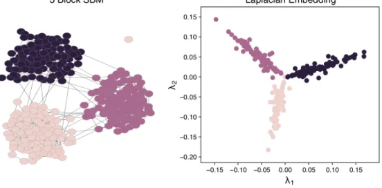
1.2 Embedding of 3 block SBM using the graph Laplacian. On the left we show the layout for a graph drawn from a 3 block non-degree cor-rected stochastic block model (planted partition model) withpin=.05and pout = .001. To the right we plot the first two eigen values of the graph Laplacian of the network, with each node colored according to the ground truth community assignment. We see that the three communities of the

model are well separated by the first two eigen values of the Laplacian. . . 6

1.3 Conceptualization of the configuration model. Given a network (left panel), we can construct the configuration model by cutting every edge in the network into two (middle panel), and then randomly re-connecting the stubs (right panel). Depending on the context, networks with multi-edges or with self loops are not allowed. See [65] for a discussion of sam-pling from the configuration model and how to avoid having self loops or

multi-edges. . . 8

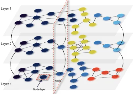
1.4 Depiction of a multilayer network with three different layers. Solid lines represent edges within each layer of the network while dashed lines represent edges across layers (interlayer edges). Node colors repre-sent communities within the network. Note that if this were to reprerepre-sent a temporal network, we have deliberately only included a few of the inter-layer edges for visibility. We have highlighted a node in the network that

extends across all three layers as well as an example of a node-layer. . . 9

1.5 The min-cut, graph partitioning problem. The goal of the min-cut problem is to partition a graph into k-parts with a minimum sized cut. A cut of a graph is the removal of edges such that subset of nodes defined by a partition are disjoint. The size of the cut is the number of edges removed (or some function thereof). In this figure, there is a cut of size 2 that separates the green nodes from the blue nodes. Note that there are other cuts of this

size in this particular example network. . . 13

1.6 TheLouvain algorithmdeveloped by Blondelet al. [27]. Each node starts in its own community, then each node is moved (in random order) into the community that gives the largest increase in modularity. Once no more moves can be identified the graph is condensed (with self loops and multiedges) on the basis of the partition and the algorithm is repeated. This

(11)

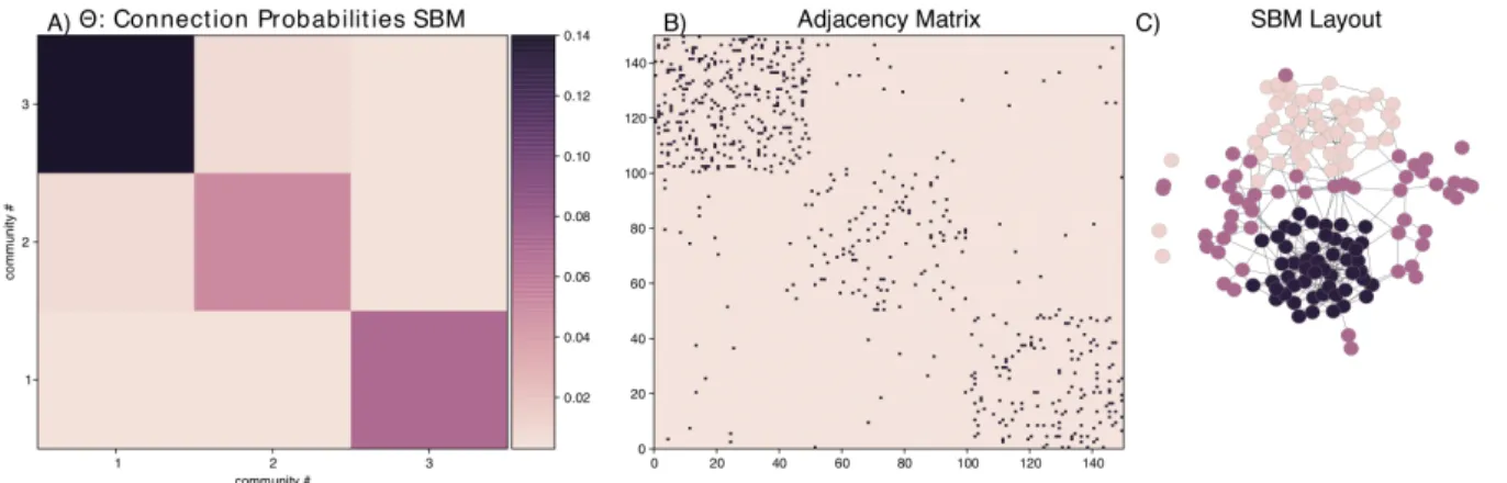
1.7 Example of a 3 community stochastic block model (without de-gree correction). A) The matrix,Θgiving the probabilities of connec-tions within and between the various communities. B) Adjacency matrix for a network sampled from this model and C) layout of the corresponding

network, colored by the block each node is assigned to. . . 22

1.8 A portion of the STRING PPI for the human genome.We have se-lected the top 83000 edges and removed all nodes with zero degree, leaving 10641 vertices. We have applied the Leiden algorithm [225], to identify 34 communities within the network, which we have denoted using the color

of the nodes. . . 37

1.9 Example of a bipartite layout.Node classes are indicated by color and shape. Edges are restricted to nodes of different classes (i.e. edges are only present between circles and triangles). This type of network commonly arises when interactions between objects are measured through a differ-ent variable of interest. Examples include the network of actors/actresses and which movies they appeared in, researchers and papers they have

pub-lished, the diseases and symptoms they express, etc. . . 46

2.1 Application of modularity-based community detection (using Lei-den method [225]) on very detectable 4 community stochastic block model. (non-degree corrected) withN = 1000,< k >= 4,ϵ =.2, community sizes = [325,325,175,175]. A)We run the Leiden algorithm

10 times for each value of γ ∈ [.1,2] in 300 evenly space intervals on a logarithmic scale. B)Layout of the network using force directed layout,

ForceAtlas2 [98], colored according to ground truth communities. . . 55

2.2 Application of Leiden [225] to the human reactome network [105,

120].We run the Leiden algorithm10times for each value ofγ ∈[.1,4]in

300evenly space intervals on a logarithmic scale. . . 55

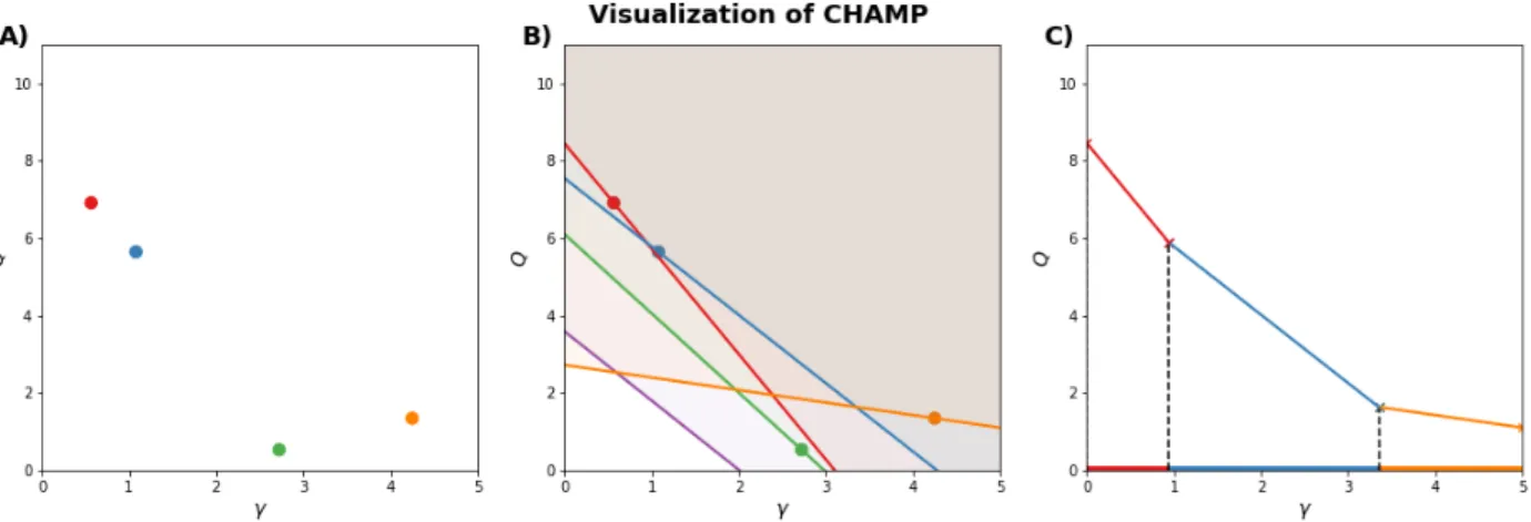
2.3 Visualization of the CHAMP algorithm. A) Each point represents a partition. The x-coordinate of the point is the resolution at which the partition was obtained by algorithm. B)We can think of each partition as defining a line. We want to to find the lines which bound the intersection of the areas above all of the lines (i.e. the region shaded brown in the figure). C)Only a fraction of the original lines will form this boundary (be in the convex hull) and each line will only optimal along some portion of the γ

domain. . . 58

2.4 Visualization of CHAMP on multilayer networks. Each planes is identified with a single multilayer partition detected using the multilayer modularity framework with set (γ,ω). Note that the surface formed by the boundary of the convex hull is piece-wise, simply connected, convex

(12)

2.5 CHAMP on the NCAA Football Network. A) ModularityQ(γ)given by Equation (3.10) versus resolution parameter γ for 50,000 runs (10%

of results displayed here) of the Louvain algorithm [27,226] at different γ on the unweighted NCAA Division I-A (2000) college football network [58,71]. Grey triangles indicate the number of communities that include≥

5nodes in each run, while the green step function shows the number in the optimal partition in each domain;B) Graphical depiction of CHAMP algo-rithm (see Section 2.3). Each line indicatesQσ(γ)given by Equation (2.2) for a particular partitionσ. Both panels show the convex hull of these lines as the dashed green piecewise-linear curve, with the transition values

rep-resented by downward triangles. . . 66

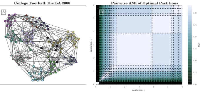
2.6 Similarity of CHAMP domains for NCAA Football. A) ForceAt-las2 [98] layout, created with [182], of the unweighted NCAA Division I-A (2000) college football network. Nodes are colored according to the dom-inant 12-community partition with the widest γ-domain γ ∈ [1.45,3.89], with node shapes and border indicating their conference labels; B) Pair-wise adjusted mutual information (N=AMI) between all partitions in the admissible subset identified by CHAMP, arranged by their corresponding γ-domains of optimality. Dashed lines indicate the transition values ofγ

identified by CHAMP. . . 67

2.7 CHAMP on the human reactome. A) ModularityQ(γ)given by Equa-tion (3.10) v. resoluEqua-tion parameterγfor20,000runs (25%of results shown) of Leiden [225] on the Human Protein Reactome network [105]. Small, grey triangles indicate the number of communities that include≥5nodes in each run, while the dark green step function shows the number in the op-timal partition in each domain. The dashed green curve is the piecewise-linear modularity function for the optimal partitions, with the transition values marked by blue triangles;B) Pairwise AMI between all partitions in the admissible subset identified by CHAMP, arranged by their correspond-ingγ-domains of optimality. Yellow stars denote the domains shown in

Figure 2.8. . . 69

2.8 Visualization of Reactome communities. ForceAtlas2 layout [98], created with [182], of the Human Reactome Network, colored according to the partitions with the three widestγ-domains of optimization identified

(13)

2.9 CHAMP applied to Caltech Facebook network. A) ModularityQ(γ)

v.γ for 100,000runs (5%of results shown) of Louvain [27, 226] on the Caltech Facebook network [227]. Orange triangles indicate the number of communities that include≥ 5nodes in each run, while the red step func-tion shows the number in the optimal partifunc-tion in each domain. The dashed green curve is the piecewise-linear modularity function for the optimal par-titions, with the transition values marked by blue triangles. The condensed layout of communities (created with [182]) here visualizes the optimal par-tition found for γ ∈ [0.908,1.09], with each pie-chart corresponding to a community, fractionally colored according to the House membership of the nodes in the community. The AMI between this partition and House labels (including the missing label) is 0.513;B) Pairwise AMI between all partitions in the admissible subset identified by CHAMP, arranged by their

correspondingγ-domains of optimality. . . 71

2.10 CHAMP on the US Senate network. A) Domains of optimization for the pruned set of partitions, colored by the number of communities within each partition. The set of partitions was generated from240,000runs of GenLouvain [101] on a600×400uniform grid over[0.3,2]×[0,2]in(γ, ω). The largest partitions are labeled “X.Y” withXthe number of communities with ≥ 5 nodes and Y the rank of the domain area (that is, in terms of size) for that given number of communities (e.g., “5.2” is the second-largest domain corresponding to 5-community partitions). The partitions of each labeled domain are visualized in Appendix 2.1;B) Weighted-average AMI of each partition with its neighboring domains’ partitions, weighted by the

length of the borders between neighboring domains. . . 72

2.11 Time-varying community structure for the U.S. Senate from 1789 to 2008 according to the (A,B) 5-community and (C,D) 8-community partitions with widest domains of optimality (see labels5.1and8.1in Fig-ure 2.10A); (A,C) The vertical axis indicates individual Senators, sorted by community label and time. The AMI reported here is the average over layers (Congresses) of the AMIs in each layer between the identified com-munities in that layer and political party labels. (This layer-averaged AMI is shown for all partitions in the convex hull over the originally searched parameter range in Figure 2.12.) (B,D) The vertical axis indicates the state of a Senator, sorted according to geographic region, and the horizontal axis

represents time (two-year Congresses). . . 74

2.12 The domains of optimality for the time-varying U.S. Senate roll-call similarity network(as in Figure 2.10), colored by the layer-averaged AMI between the political-party affiliations of Senators and the community

(14)

2.13 Size and consistency of the CHAMP sets for reactome network[105,

120]. A)The total size of the CHAMP set for each partition ensemble ofr runs, averaged over 10 trials. Size of baseline set of all partitions indicated by gold star. B)The average AMI between the CHAMP set for each par-tition ensemble ofrruns and the baseline ensemble, weighted by the size of the domain, and averaged over 10 trials (see Equation 2.8). Baseline

partition has average AMI of 1 by construction. . . 76

2.14 Exploring the stability of the CHAMP sets for reactome network[105,

120]. A)We compute the AMI for the intersection of each domain between the partitions for the baseline set of all partitions, and each individual set withrruns. We have averaged the individual step functions over 10 inde-pendent trails, each withrruns.B)Location of transitions between dom-inant domains for each of the 10 trials with 102400 runs of Leiden, uni-formly spaced acrossγ = [0,4], as well as the transitions for the baseline

combined set (1621000 total runs) shown in red. . . 77

3.1 Example representation of a factor graph. Each node is of one of two classes: variables represented by green circles or factors, represented by colored squares. Each variable node can occupy one of several states. Each factors node one more more of the variables as input to determine its value. The overall probability of a given state of the model is the product

over all of the factor nodes. . . 84

3.2 Schematic of modularity belief propagation.We have split the con-tributions to the modularity into two kinds of interactions: strong interac-tions represented by edges in the original graph (shown as dark, solid lines in figure) and weaker, all-to-all connections given by the null model term (shown as dashed lines). Beliefs (shown as arrows) are summed from all

interacting nodes except the one who is receiving the message (far right node). . . . 88

3.3 Demonstration ofmultimodbpon two realizations of the origi-nal SBM model (non-degree corrected).From left to right, the plots show the retrieval modularity, number of iterations to convergence, and the AMI of the retrieval partition with known community assignments and the effective number of communities. (a) 4 community SBM with n = 1000, ϵ = pout_pin = .1, cavg = 4, and even community sizes and (b)and 4 community SBM withn= 1000,ϵ=.1,cavg = 4, with uneven community sizes (ν = [300,200,300,200]). For each network we also show the perfor-mance of thesbmbpwith parameters for the SBM supplied (middle plot,

dotted black line. See Section 3.3.1 for details ofsbmbpmethod.) . . . 95

3.4 Performance ofmultimodbpandsbmbpover many LFR bench-mark realizations with a range of values for the mixing parame-terµ.Each point represents an average over 100 realizations of LFR with 1000 nodes, an average degree of 3 (with a max of 10), and other

(15)

3.5 Testingmultimodbpon the 2000-2001 Division I-A College Foot-ball network [58,71]. A)The average number of iterations until con-vergence in the retrieval phase across a range ofγ values. B)The average number of communities detected in the retrieval phase asγ increases and the corresponding adjusted mutual information (AMI) of those partitions. C)ForceAtlas2 [98] layout of the football network with each node colored according to a partition identified usingγ = 3.0, demonstrating excellent

alignment to the conference structure. . . 99

3.6 Performance characteristics of the algorithm for 3 different val-ues of γ on the 2000-2001 NCAA Division I-A College football network. A)Although all three values ofγproduce a wide retrieval phase, the communities identified within each retrieval phase are different. B) The number of non-redundant communities is higher asγ increases with γ = 3 producing the number of communities that lines up well with the ground truth (the conferences) in this example, with C) showing corre-sponding higher values of AMI for γ = 3. Horizontal black dashed line shows thatsbmbpidentifies correct number of communities inB)but has

less agreement with the known conference structure of the network. . . 99

3.7 Accuracy of the multilayer modbp algorithm on a DSBM.We test multimodbpacross different values of model parametersϵ, andη(x and y axes respectively) and formultimodbpparametersγandω(moving hori-zontally and vertically vertically across panels). For these generated

net-works,N = 250,nlayers = 20,c= 10, andqtrue= 2. . . 101

3.8 Graphical representation of the community structures for net-works samples from different interlayer topologies available with the multilayer-generative model in [21].In each subfigure, each row represents a particular node, with each column representing a layer of the network. Each node-layer is colored according to its multilayer partition. Thus we can see how the different communities persist across the layers of

(16)

3.9 (Previous page.) Comparison ofmultimodb withGenLouvainon multilayer benchmarks. We compare the performance ofmultimodb (top rows of each panel) andGenLouvain[104] (bottom row of each panel) across a range of multilayer benchmark networks developed by Bazzi et al. [21]. For each model we vary bothµ, the intralayer mixing parame-ter (strength of communities) denoted by the different markers and colors. From left to right, across the subfigures, we vary the persistence of com-munities across layers from p = .5 to p = 1.0. Each points represents the average ⟨AMI⟩ over 100 independent realizations of the model. A) Temporal network topology with ordered layers and interlayer connections only present between adjacent layers. Multilayer community partitions are drawn from Dirichlet distribution withθ = 1, nset = 5, andq = 1and in-tralayer edges are samples from a DCSB with : ηk=−2, kmax= 30, kmin=

3. Each network has 100 node-layers in each layer with 150 layers for a total of 15000 node-layers. B)Uniform multiplex multilayer network with un-ordered layers and all to all interlayer connections among identified node-layers across all node-layers. Multilayer partitions are sampled from Dirichlet distribution withθ = 1, nset = 10, andq = 1and intralayer connections are drawn from DCSB withηk=−2, kmin = 3, andkmax = 150. Each net-work has 1000 node-layers in each layer with 15 layers for a total of 15000 node-layers. C)Block multiplex model with the same parameters as the uniform multiplex models however we introduce a discontinuity between

each block of 5 layers where community labels are completely independent. . . 107

3.10 Detectability of communities in the uniform multiplex bench-marking network (withp =.85) asµis varied. We plot the average

⟨AMI⟩ of the detected communities for bothmultimodbp (solid red line) and forGenLouvain(solid blue line). We also show the average modular-ity of the partitions identified byGenLouvain(dashed blue line) as well as

percentage of trials that converged to a non-trivial solution formultimodbp . . . . 108

3.11 Application ofmultimodbpto US Senate voting network.We ran multimodbpon the US Senate voting similarity network comprised of 1884 Senators across the first 110 Congresses [155,242].A)The relationship be-tween the retrieval modularity (x-axis) and the Bethe free energy is given by equation Eq 3.35. The Bethe free energy correlates strongly with mod-ularity of a partition, and the partitions with the lowest free energy tend to correspond best with the underlying party structure. B)We examined the distribution of the average Senator entropy for each Congress (layer) in the network. Inset graphs depict how changes in average entropy correspond with network structure and the overall level of polarization within the net-work. Node size depicts the average entropy level of Senators with “high

(17)

3.12 Several visualizations of the Lazega Lawyer network [127]. On the right we show several characteristics of partitions identified with mul-timodbp at various values of γ (x-axes) and ω (y-axes). In the top row, from left to right, we show how many times the algorithm converged over 10 runs at differentβvalues, the number of communities identified by the best run for each set of parameters (based on lowest Bethe free energy), and the average entropy of the marginals across all of the nodes for each of these partitions. In the next two rows we show the AMI of the identi-fied partition within a single-layer and a speciidenti-fied metadata attribute. For example in the left most panel of the second row, we show how the “prac-tice” (which type of law practiced by each node) attribute lines up with the partitioning of work layer. To the right inB)we show the three lay-ers of the network (advice, work, friends) colored by two of the metadata attributes, practice (which specialty of law each person is involved in) and office (which is the location the person works in). Showing the partitions in this manner demonstrates how different metadata attributes affect the community structure in the different layers and how this is best captured

bymultimodbpfor different values ofγ andω. . . 111

4.1 Application of univariate approach to DDR pathways and com-parison against all genesA) We show the distribution of Tumor muta-tional burdens (TMB) for all samples with a mutation in each of the DNA Damage Repair (DDR) pathways. Dashed line shows the median TMB for all TCGA samples (including those with mutations in the DDR pathways) with light blue line showing the interquartile range. Mann-Whitney U p-values are calculated by comparing the distribution of TMB for samples with any mutation in the genes that define a pathway (counting only once if they have multiple mutations) to the distribution of all samples, again including those with mutations in the DDR pathway. B) Distribution of Mann-Whitney U test p-values (without multiple test correction) across all genes in TCGA. For each gene MWU test compares distribution of TMB values for samples with a mutation in the gene vs all samples in cohort. C) Distribution of mean TMB values for mutated sample set for each gene

compared with the overall mean TMB for the cohort (dashed black line). . . 124

4.2 Comparison of mutation frequency with mean TMB of mutated sample set. Gene level mutation frequency (x-axis) plotted against the mean TMB for all samples with a mutation in each gene. (y-axis) for the PMECA)and the TCGAB). Each scatter point represents a unique gene in the dataset, with DNA Damage Repair genes starred and colored according to their pathway (see legend in panel A). Dashed horizontal lines depict the threshold for high TMB(> 10)as well as the mean TMB for all samples within the data set (lower line in each panel). Regression curve show slight negative relationship between mutation frequency and the median level of

(18)

4.3 Schematic representation of converting our mutational data in matrix from, B to a bipartite network. The two classes of nodes are the genes and the samples. Each sample is connected to a gene if that sam-ple has a mutation within that gene. For simplicity, we consider an un-weighted bipartite network since it is rare for a sample to have multiple mutations in the same gene. Far right panel depicts the friendship para-dox for a randomly generated (non-bipartite) network using a common, synthetic benchmark model (Lancichinetti, Fortunato, & Radicchi, 2008) . Each scatter plot represents a node in the network, with the x-axis show-ing the node’s degree, and the y-axis showshow-ing the average neighbor degree. The scatter plots that are above the y=x line (dashed orange line) have a higher average neighbor degree than their own degree. We see that this is

the case for most nodes in the network. . . 127

4.4 Sampling from the bipartite configuration model A)Depiction of the configuration null model for a given network. Edges are ‘cut’ in two leaving stubs, which can be connected to any other stub as long as the bi-partite structure is maintained. In the configuration model, each valid ar-rangement is equally likely to occur. B)We can sample from the configu-ration model by repeated rewiring of the network. The samples from the model will be independent as long as a sufficient number of rewires has

occurred between each sample. . . 130

4.5 Sampling the distribution of mean TMBs from the bipartite null model. Each blue step function represents the empirical cumulative dis-tribution function for the TMB of all samples with a mutation in the se-lected gene (MSH3) in a single network drawn from the null model. The red line shows the observed distribution of TMB and the inset shows the dis-tribution of the means of each set of sampled TMBs with a fitted Gaussian overlaid. The red dashed line in the inset represents the observed mean

TMB for that gene. . . 131

4.6 Application of bipartite configuration test to the DNA Damage Repair pathways in the TCGA data. Each figure shows the observed cumulative distribution of TMB for samples with any mutation in the genes of the specified pathway (with samples with multiple mutations counted only once) by the red solid line. The blue line shows the average cumu-lative distribution across 500 sampled networks, with the light blue band showing the 99% confidence interval. The horizontal line at y = .5 de-notes the median TMB for the distributions. The inset figure in each panel shows a histogram of the means of the sampled distributions of TMB for samples with a mutation in the corresponding DDR pathway. The verti-cal red dashed line depicts the observed mean TMB in the actual data set. Z-scores were constructed by comparing the observed mean TMB to the

(19)

4.7 Comparisons of permutation test applied to DDR genes. A)We compare z-scores obtained for each of the DDR genes (solid dots) and the DDR pathways (open circles) using both the PMEC dataset (x-axis) as well as the TCGA mutation data (y-axis). Solid gray lines indicate boundaries for ap < .05 significance threshold for each test. B)We compare the z-scores obtained for the permutation test in the TCGA data with the p-values for the corresponding Mann-Whitney U test in the same dataset. Genes are

colored in both plots according to their DDR pathway. . . 134

4.8 Characterization of network permutation test Distributions of p-values for theA)Mann-Whitney U test as well as theB)network permuta-tion test applied to all18,000genes in the TCGA dataset.C)Z-score values and protein length (number of amino acids) show no relationship.D) Mu-tation frequency for each gene in TCGA plotted against its z-score based on

the permutation test. . . 135

4.9 Gene Ontology Enrichment analysis for genes with the lowest z-scores. Bars represent the−log₁₀of the p-values for the corresponding GO term with multiple test correction applied (using Bonferroni multiple

test correction). . . 136

4.10 Effect of Low Zscore DDR mutations on survival for the IMVigor dataset. A)Splitting the samples into groups based on high(>10)or low TMB(< 10)and mutated or WT for the low z-score DNA Damage Repair Genes. Samples are groupled based on whether or not they had a mutation in a low z-score DDR gene. We tested a Cox proportional hazard model for differences in overall survival between these four groups. B)Forest plot showing the estimated coefficients for a CPH model testing jointly testing TMB, mutation in low-zscore DDR genes, as well as an interaction term be-tween the two variables (denoted by DDRlow:highTMB). We note here that TMB is treated as a continuous variable.C)andD)show the percentage of clinical response rates across the samples segregated by low TMB with no mutation in low z-score DDR, low TMB with a mutation, high TMB with no mutation, and high TMB with a mutation in order. Red bars denote the percentage of samples in each group that had a complete or partial re-sponse while blue bars denote the fraction that had stable or progressive

disease. P-values were assessed using Fisher’s exact test. . . 138

4.11 Effect of Low z-score DDR mutations on survival for the Sam-stein dataset. A)Splitting the samples into groups based on high(>10)

or low TMB(< 10)and mutated or WT for the low z-score DNA Damage Repair Genes. We group samples based on whether or not they had a muta-tion in a low z-score DDR gene. We tested a Cox propormuta-tional hazard model for differences in overall survival between these four groups, each treated as a dummy variable. B)Forest plot showing the estimated coefficients for a CPH model testing jointly testing TMB, mutation in low-zscore DDR genes, as well as an interaction term between the two variables (denoted by DDRlow:highTMB). We note here that TMB is treated as a continuous

(20)

4.12 Splitting DDR genes on the basis of z-score. We split the DDR genes on the basis of having a high (>0) or low (<0) z-score for both the IMVigor and the Samsteinet al.datasets. Here we show the distribution of z-scores

as well as which genes were placed in each category. . . 145

13 Visualizations of partitions labeled in white in Figure 2.10.A, with Senators grouped according to their state. The listed AMI is the average over layers of the AMI in each layer (Congress) between the communi-ties and political party affiliations for that Congress. Partitions are labeled “X.Y” withXthe number of communities with≥5 nodes andY the rank

of the domain area for that number of communities. . . 148

14 (Previous page.) Visualizations of partitions labeled in white in Figure 2.10.A, with Senators sorted by their most frequent community label (with the labels sorted by last appearance in time), and within com-munities by first appearance. The listed AMI is the average over layers of the AMI in each layer (Congress) between the communities and political

party affiliations in that Congress. . . 150

15 Stability boundary for Erdös-Rényi graph with weights assigned randomly from aN(µ, σ =.5)normal distribution. Left three plots depict convergence curves of the algorithm for three different means of the normally distributed edge weights (µ=1,2, and 3 respectively). Each curve represents the average over 10 realizations of the ER random graph. The unweighted prediction forβ∗ is given by the black dashed line, while the weight adjusted prediction is given by the dashed green line. On far right plotβ∗was empirically determined for several different mean weights (red

line) and compared with the predicted values (blue line) showing good agreement. . 155

16 Stability boundary for 2 community stochastic block model graph with weights assigned randomly from aN(µ, σ =.5)normal dis-tribution. SBM’s had n = 200 nodes with mean degree, c = 6, and ϵ = pout

pin = .1. Each convergence curve was averaged over 10 realizations

of the SBM model with different means of the normally distributed edge weights (µ =1,2, and 3 respectively). The unweighted prediction forβ∗is given by the black dashed line, while the weight adjusted prediction is given by the dashed green line. Red curve shows the adjusted mutual information with the underlying ground truth. On far right plotβ∗was empirically de-termined for several different mean weights (red line) and compared with

(21)

17 Stability boundary for 2 community unweighted multilayer dy-namic stochastic block model graph. Network had n = 100 node within each layer with mean degreec = 6and ϵ = pout

pin = .1. Each

con-vergence curve was averaged over 10 realizations of the SBM model with the algorithm run with different interlayer edge couplings (ω =0, 1, and 2 respectively). The unweighted prediction for β∗ is given by the black dashed line, while the weight adjusted prediction is given by the dashed green line. Red curve shows the adjusted mutual information with the un-derlying ground truth. In the far right plotβ∗was empirically determined for several different mean weights (red line) and compared with the

pre-dicted values (blue line) showing good agreement. . . 156

18 Effect of varying γ with q remaining fixedWe compare the perfor-mance of the algorithm for a wide range ofγ values in the event that the number of communities is fixed at the correct number (q = 4). Here we do

not allowqto float as described in Section 3.5.2 . . . 157

19 Attempting to select the appropriate value of q on the American football network.Using the method recommended by Zhang and Moore to select the appropriate value of q for the American NCAA Div-IA Col-lege Football Network [58,71]. Each colored line corresponds to running modbp for a given value ofq across a window of β around β∗(q) (shown by black dashed line). Using this method would suggest an appropriate q ∈[6−8]depending on the threshold selected. We note that here, we do not collapse community labels as described in Section 3.5.2; for each run a single fixed value ofqis used as well as the default resolution (γ = 1). AMI

with the school conferences is denoted for eachqby the colored ”X”. . . 157

20 Scanning theβdomain for the US Senate Rollcall dataset.We run multimodbpon the US Senate Voting similarity network [242], using the KNN (k=10) as described in Section 3.3.2 of the main text. We ran multi-modbpfor a maximum of 4000 iterations across 100 evenly spaced values of β ∈ [0,1]. For each value of β we ran multimodbp5 different times. We show that Shiet al’s approach to selectingβ∗ [208] identifies regions where the algorithm is in the retrieval phase (i.econverges to non-trivial partitions). Vertical dashed black lines show calculated value forβ∗(q)for q = [4,6,8,10,12,14]. Vertical blue and red bars denote the percentage of runs for that value ofβ that ultimately converged (percentage is shown by the proportion of the space under the number of iterations curve occupied by the bar). Bar color denotes whether the identified partitions were trivial (ψi

t = 1q∀i, t) We see that several of these lie within the observed retrieval

(22)

21 Fragmentation of identified communities across layers. Demon-stration of layer ”splitting” on the multilayer dynamic stochastic block model (DSBM). Left shows the ground truth planted community assignments while the right shows the communities identified by multimodbp without the cross layer assignment procedure. We reiterate that this cross layer label permuting preserves all identified structure within a layer and always

re-sults in higher modularity. . . 159

22 multimodbpapplied to the US Senate Voting similarity network [242]. Left: AMI of identified partitions with the political party labels using multimodbp across a range ofγ (x-axis) and ω values. Right: the number of communities identified by the algorithm as a function of the

parameters(γ, ω). . . 159

23 Community structure for lowest free energy partitions identi-fied bymultimodbp.Top identified partitions based on minimization of the Bethe free energy on the US Senate voting similarity network. In each, each row represents the Senator for a particular State, organized by region, while the x-axis denotes the year of each Congress. Nodes are colored ac-cording to their identified partition, while the top left figure is colored by

the political party affiliation of each senator. . . 160

24 Multiplex benchmark without spectral initialization and only us-ing spectral method. Top row: the performance of multimodbp on the uniform multiplex network (as specified in Section 3.3.2 of the main text)withoutthe spectral initialization detailed in the main text. Perfor-mance of the algorithm at higher omega trails off abruptly. For comparison withmultimodbpwith spectral initialization, see Figure 3.9 in main text. Bottom row: performance of just the spectral initialization (without mul-timodbp). The spectral initialization’s performance tends to be better at

higher values of omega, complementing the deficiencies inmultimodbp. . . 161

25 Comparson of general characteristics of PMEC vs TCGA. AScatter of the short mutation (SNV+indel) frequency for the DDR genes in PMEC (x-axis) vs TCGA(y-axis). B) Scatter of the CNV frequency for the DDR genes in PMEC (x-axis) vs TCGA(y-axis). C)Scatter of median TMB levels by cancer type for PMEC vs TCGA.D)Venn diagram of overlap between

broad cancer types in TCGA vs PMEC. . . 163

26 Permutation test z-scores for all PMEC genes. AWe scatter the z-scores for the permutation test for the 481 genes in PMEC for TCGA vs PMEC. Note that scores for the TCGA dataset were derived using the full 18K genes.B)We also show how the−log₁₀p-value for the Mann-Whitney

(23)

27 Testing for association with survival in samples with a high z-score DDR mutation. A)Kaplan-Meyer curve for IMVigor samples binned according to high vs low TMB and mutated or WT in high z-score DDR genes.B)Cox-proportional hazard model for IMVigor fitting TMB (as con-tinuous variable), along with mutation in high z-score DDR genes, as well as a cross term between TMB and mutation in high z-score DDR genes.C)

andD)Analogous plots for the Samsteinet al.dataset. . . 165

28 Testing for association with survival in samples with a low MWU score DDR mutations. AKaplan-Meyer curve for Samsteinet al. sam-ples binned according to high vs low TMB and mutated or WT in low MWU test DDR genes. B)Cox-proportional hazard model for IMVigor fitting TMB (as continuous variable), along with mutation in low MWU test DDR genes, as well as a cross term between TMB and mutation in low MWU test

(24)

LIST OF ABBREVIATIONS AND NOTATION

G(V,E) Network containing set of nodesVwith the set of edgesE

A Network adjacency matrix

D Diagonal degree matrix:diag(ki)

L The graph Laplacian matrix:D−A

N Number of nodes in a network

M Number of edges in a network

ki The degree (or strength) of nodei.

c Vector of node-to-community assignments

ci The community assignment of nodei

pk The degree distribution of the network.

δx,y Indicator function onx=y. Assumes value of1ifx=yotherwise0. ER(N,M) Erdős-Renyi network model withN nodes andM edges.

SBM Stochastic Block Model

p_in Within-community edge probability under planted partition SBM pout Between-community edge probability under planted partition SBM

CHAMP Convex Hull of Admissible Modularity Partitions (see Chapter 2)

(25)

CHAPTER 1: INTRODUCTION TO NETWORKS, COMMUNITY

DETECTION, AND APPLICATIONS TO ONCOLOGY

We begin this thesis with an overview of the basic concepts underpinning the main ideas

presented in this work, including networks and community detection with a focus on

personalized medicine. Advances in networks science have arisen from a plethora of fields:

sociology, physics, statistics, pure and applied mathematics, computer science, and many others.

This convergence of problems arising in radically disparate domains with a common set of

solutions is one of the most exciting parts of working in the field. However, it can make it difficult

for the casual reader to find an appropriate entry point into the discipline without getting drawn

into other minutia. In this introductory chapter, we hope to provide enough of a flavor of this

fascinating field to keep the reader engaged, and to provide a foothold for accessing this deep and

diverse body of work. For the interested reader who wishes to dive deeper, we recommend

Newman’sNetworks[167] or Kolaczyk’sStatistical Analysis of Network Data[117], both of

which provide a hearty, self encapsulated introduction to networks. We begin by giving an

account of what networks are and why they arise in so many different contexts. We discuss

community detection in networks, detailing the different approaches and the philosophies

underpinning them. Finally, we conclude the chapter by giving an overview of how network

approaches, including (but not limited to) community detection have been used in the field of

cancer genomics. We segue into the next chapter by giving an overview of the rest of the thesis

and summarizing the main contributions of this work.

1.1 Networks

We conceptualize a network as an abstract collection of objects and relationships between

those objects. We refer to the “objects” as nodes or vertices and the relationships as edges. In

(26)

typically represent pairwise interactions, involving two nodes only¹. We assign each node an

arbitrary index,i∈1, . . . , N and denote a specific edge by the pair of nodes it involves:(i, j)∈ E. Our definition of a network is quite simple and quite broad; hence there are many systems in the

real world that can be conceptualized as networks:

G = ({genes},{physically interact with each other})

= ({cities},{connected via a road})

= ({researchers},{have published a paper together})

. . .

All of these have a notion of individual entities (nodes) who come together through

interactions (edges) to form a more complex system. We typically visualize a network by drawing

circles for the nodes and lines connecting the circles for the edges as demonstrated in Figure 1.1,

where we have assigned each node a coordinate in 2D space based on an algorithm to reveal

clusters, although the layout is just one of infinitely many we could have chosen to show this

network. It is merely a representation of the underlying structure and not itself intrinsic to that

structure. Such visualizations can make us think of each network as living in 2D or 3D space;

however, they are much higher dimensional objects themselves as each network can have up to (_N

2 )

=N(N −1)/2possible edges and thus can have the same number of degrees of freedom. In most networks of interest, there are many correlations between edges that can vary across the

network, greatly reducing the complexity of the information content within the network.

Networks can range in scale from tens to hundreds of millions of nodes², and the appropriate

visualization will depend on the size of the network as well as the density of edges.

Another way networks are commonly represented, especially to perform computations, is

¹Higher order networks (e.g.involving triplets or quartets) are called hypergraphs

(27)

Figure 1.1: The famous Zachary karate club network. [255]. Each of the 34 nodes represents a member of the karate dojo Zachary was studying over several years, while edges represent whether or not Zachary ob-served consistent social interactions between the members outside of the official functions of the club. During the course of the the study, a disagreement between the leaders caused a split into two different clubs.

by an adjacency matrix, denotedAwhere:

Aij =

      

1 (i, j)∈ E

0 otherwise

. (1.1)

For a network withN nodes,Awill be anN ×N binary matrix³ (which we also can denote A∈ {0,1}N×N). As any reindexing of the nodes will result in a permutation of the rows and columns ofA, there are many adjacency matrices that can correspond to the same underlying network. The adjacency matrix is computationally useful because it allows us to use both the

theoretical and computational tools of linear algebra to address questions concerning networks.

Networks theory has found application in nearly all applied sciences. Much of the early

work in the study of networks arose in the context of sociology, focusing on the empirical

distribution of node-level metrics of observed networks as well as developing simple models of

network formation to understand how those distributions could have arisen. For example, one of

the major network quantities of interest is the distribution of the degrees of a network. The degree

(28)

of a node,k, is the number of other nodes attached to it: ki = ∑

jAij. The degree distribution of a network, denotedpk, is the probability that a randomly chosen node has degree,k(i.e. the

number of nodes with degree,kdivided by the total number of nodes in the network). In most social networks, it was found that often there are a few high degree nodes, referred to ashubs, that

play important roles in the network. This simple fact concerning the distribution of the degrees

explains the surprisingsmall-worldeffect described by Milgram [150]: despite the fact that there

are almost 7 billion people in the world, any two randomly selected people are separated (with

high likelihood) by a path of no less than six hops along edges within the networks. This same

phenomenon accounts for the fact that even though there are tens of thousands of airports in the

world, in most cases you can fly commercially between any two of them with only 1 or 2 layovers.

These structural facts have implications for a number of other fields as well. Both sociologists as

well as epidemiologists are interested in how phenomenon propagate themselves over a network:

mathematical models of how news, fashion trends, or voting preferences spread on a network will

have similar considerations to understanding an epidemic of a deadly disease.

Many domains in the biological sciences have also been impacted by developments in

network theory, providing researchers with the ability to take a systems-level approach. From

understanding the organization and functioning of the human brain at multiple structural levels;

to the modeling of chromatin folding and disruption [169]; to assembling and interpreting the

human genome [42]; All of these and many more systems can be tackled with the tools of

networks. Recently, as we shall overview in Section 1.3, the field of oncology has been

transformed by the exciting merger of large scale genomics data with the development of

networks-based approaches.

There are many possible extensions of the basic network described above that allow one to

capture more of the complexity of systems in the real world. One could allow for different

strengths of interactions, placing weights on the edges (weighted networks), or allow for the

interactions to have a directionality (directed network). We could also allow for multiple edges to

exist between pairs of nodes (multigraph) or allow for different kinds of edges (multilayer

network). For most of these, the operational representations of the network can be extended in a

natural way to make use of the available tools. For instance, in the case of the weighted networks,

(29)

complexity added by the weights. In other cases, a more careful handling is required; throughout

the work we attempt to specify the kind of network we are using in each case when special

considerations are required. We provide a greater explanation in the next few subsections on

several needed concepts including the treatment of networks with multiple layers (multilayer), as

these are the focus of much of this thesis.

1.1.1 T G L

Earlier, we saw how the adjacency matrix,A, encodes the structural connectivity of the

network in a relatively straightforward way. We introduce here the concept of the graph

Laplacian, another matrix encoding the same structural information that arises in a number of

contexts, especially in considering the dynamics of processes occurring on the graph. The graph

Laplacian is a discrete version of the Laplacian operator∇2_{that provides a notion of smoothness}

for a function over a graph.

If we have a function,f, defined on each node byfi, we can derive the graph Laplacian by considering how different the values off are across neighboring nodes of the network:

||f||2_G =∑

ij

(fi−fj)2Aij . (1.2)

This equation then provides us with a simple notion of what it means for a function to be

smooth across a network. If differences in the value offfor neighboring nodes is usually small,

then||f||2_Gwill also be small. If we rewrite this equation as follows:

||f||2_G=∑

ij

(fi−fj)2Aij

=∑

ij

f_i2Aij +f_j2Aij −2fifjAij

= 2(∑

ij

f_i2Dij− ∑

ij

fifjAij)

= 2(fTDf−fTAf)

(30)

where we have introduced the degree diagonal matrixD:

Dij =

      

ki If i=j

0 otherwise

, (1.4)

and have defined the graph Laplacian,L=D−A. Thus the graph Laplacian can be thought of as

a discrete difference operator on the graph. The graph Laplacian appears in many places in graph

theory, including the identification of the minimum spanning tree and in regularization for

machine learning approaches to graph structured data. The eigenvalues of the graph Laplacian

also contain information about the community structure of the graph as can be seen in Figure 1.2.

Figure 1.2: Embedding of 3 block SBM using the graph Laplacian. On the left we show the layout for a

graph drawn from a 3 block non-degree corrected stochastic block model (planted partition model) withpin = .05andpout =.001. To the right we plot the first two eigen values of the graph Laplacian of the network, with

each node colored according to the ground truth community assignment. We see that the three communities of the model are well separated by the first two eigen values of the Laplacian.

1.1.2 M N

Much of network science has centered around the development of models of networks

that capture aspects of real world networks. For instance, the Watts-Strogatz’s “small world”

model attempts to generate networks with relatively short paths between possible pairs of nodes

(31)

fat-tailed, power law degree distribution,⁴ which is common in many real world networks [4] ⁵.

Here we briefly introduce the concept of a network model and describe the Erdős-Rényi model

and the configuration model, both of which will be useful throughout this thesis.

In broad terms, a random network model defines a distribution over the space of possible

networks one could observe. Often we use a model to look at how certain statistics behave over an

ensemble of networks drawn randomly from our model. The Erdős-Rényi (ER) model is one of

the simplest random network models: we allot equal probability weight to every network that has

a given number of nodes and a specified number of edges. We denote this distribution of

networks by :ER(N, M). Instead of specifying a fixed number of edges, it is often more useful (and analytically tractable) to specify the independent and identically distributed (IID)

probability each edge has of occurring,p, written asER(N, p). In this case, the expected number of edges isM =p×(N₂). For a large enoughN the two models converge to each other. As each edge has an equal probability of being selected, the degree distribution for each node is simply the

binomial distribution:pk∝ (_n₋₁

k )

pk(1−p)n−1−k.

Another random graph model that will appear several times in this work is the

configuration model. The configuration model is interesting in that the specified parameter is the

degree distribution itself,pk. The configuration model assigns equal probability to every network with the specified degree distribution (and zero to all others). Typically, we can use the

configuration model to interrogate whether or not the properties we have observed in a real world

distribution are independent from its degree distribution. Given a network, one way to construct

the configuration model is to cut each edge in two, leaving a corresponding stub on each node.

The configuration model is formed by placing equal weight on all of the possible ways of

reconnecting the stubs, as illustrated in figure 1.3. We can calculate the probability of there being

an edge between any two nodes,iandj, under the configuration model. Each stub has an equal probability of connecting with any other stub in the network. For a given stub on nodei, there are

kjstubs on nodejfor it to connect to; therefore the probability of it being connected to a stub on

⁴A power law distribution follows the following functional form:P(X =x)∝x−α. Typically2< α <3

(32)

Figure 1.3: Conceptualization of the configuration model. Given a network (left panel), we can construct the configuration model by cutting every edge in the network into two (middle panel), and then randomly re-connecting the stubs (right panel). Depending on the context, networks with multi-edges or with self loops are not allowed. See [65] for a discussion of sampling from the configuration model and how to avoid having self loops or multi-edges.

nodejis kj

2m−1. And since there arekiindependent chances of a stub on nodeiconnecting to a stub on nodej, then the total probability of an edge between the two is given by kikj

2m−1 (≈ kikj

2m for

large enoughm). There are many other network models that attempt to capture various aspects of observed networks. In section 1.2, we discuss a few more complicated models that attempt to

capture higher order structure in the network by defining a notion of “communities”.

1.1.3 I M N

In recent years, there has been great interest in extending the traditional network models

to encompass more complexity that can better reflect a variety of systems. Specifically, in many

systems, interactions between objects can vary over time, be of multiple types, or other

complexities. For example, in a network of social actors, there could be multiple types of

relationships that are captured: are friends, have worked on a project together, are family

members, etc. We can incorporate this kind of structure by stratifying the nodes of the network

across multiple “layers” or dimensions. A multilayer network allows us to represent multiple

types of relationships between nodes in a unified way.⁶ Throughout this work, we have adapted

the multilayer notation and terminology from Ref. [114].

In the multilayer formulation, all edges representing a certain kind of relationship are

(33)

present within a layer. We show a depiction of such a network in Figure 1.4. In addition, we can

allow for relationships for nodes in different layers encoded by the interlayer edges (shown by

dashed lines in Figure 1.4). Typically, the interlayer edges encode the persistence of identity of

Figure 1.4: Depiction of a multilayer network with three different layers. Solid lines represent edges

within each layer of the network while dashed lines represent edges across layers (interlayer edges). Node col-ors represent communities within the network. Note that if this were to represent a temporal network, we have deliberately only included a few of the interlayer edges for visibility. We have highlighted a node in the network that extends across all three layers as well as an example of a node-layer.

nodes across the various layers. For example, consider a multilayer where each layer represents

observed email correspondence between the executives of a firm within a given time frame. Each

executive would be represented in each layer by a specific node, with nodes in adjacent layers

(representing neighboring time frames) connected by an interlayer edge. To distinguish between

the single node or object of analysis across all layers, and its representation in any given layer, we

refer to a particular node as it exists within a layer as a “node-layer”.

There are several ways to encode a multilayer network. In the single-layer (also referred

to as monoplex) network, we represented the edges between all pairs of nodes through a single,

(34)

M∈RN×N×L, where L is the number of layers in the multilayer network.⁷ It is common to flattenMinto anA∈RN L×N L, “supra-adjacency” matrix, where each nodek∈[1, N]is identified with node-layers indexed{i, i+N, . . . , i+N(L−1)}. We use the notationi∼=jto denote that two node-layers are identified with the same node. Typically we index the node-layers

such thati∼=i+N ∼=...∼=i+N ∗(L−1). We use the “supra-adjacency” notation in the rest of the paper andi, j, kto refer to node-layers in the network unless otherwise specified. We also use a single vector to keep track of which layer each node-layer resides in:⃗l= [l1, ..., lN L]where

li ∈[1, L]specifies the layer that node-layeriis in. We useVlito denote the set of node-layers in

layerli(i.e.nodes in the same layer asiincludingiitself). In addition to the edges within each of the layers, we also have to specify the overall topology across the layers. We encode the interlayer

topology through the matrixC∈RN∗L×N∗L. We only allow elements ofCto be non-zero if the corresponding node-layers are in different layers :Cij = 0ifli =lj. Typically each node-layer will be connected to a subset of the other node-layers corresponding to the same node in different

layers, but C can represent any number of interlayer topologies.

There are many different kinds of multilayer topologies that could be encoded by the

supra-adjacency format. Two of the most common types are the (discrete layer) temporal

topology and the multiplex topology. In the temporal topology, we have an inherent ordering of

the layers, usually representing observations of our system over time. Node-layers are typically

connected by interlayer edges only for adjacent layers. Examples of temporal networks include

observed functional connectivity patterns across regions in the brain at different times while

performing a cognitive task [19] or observed patient referral patterns for a group of physicians

across different years [228]. Multilayer networks can also encode a multiplex topology. Each

layer represents a different kind of relationship; however, there is no inherent ordering on the

layers. Identified node-layers are connected across all possible pairs of layers. Examples of

multiplex multilayer networks could include an observed social network where edges are

constructed separately from phone, text, and face-to-face contact information [94], or perhaps a

transportation network of the London underground where different lines connecting various

(35)

stops are represented by different layers[196]. It is also possible to have a multilayer network

with both multiplex and temporal topology. In these, we can imagine several “dimensions” of

layers, with each layer being described by multiple aspect labels. For example we could observe a

multiplexed social network over many time frames.

The earliest approaches to multilayer network analysis attempted to characterize them on

the basis of well established single layer metrics. For example, to detect community structure,

researchers attempted to apply single layer tools on each layer of the network individually, and

then perform post-hoc alignment of the different layers [15]. There have also been attempts to

map multilayer networks into a monoplex network and apply existing single layer methods. [25].

There are several different ways to collapse a multilayer network into a single layer network (for

instance an using an OR operation on the existence of any edges or requiring an edge to be

present in every layer [218]). While it is possible that the loss of information from collapsing does

not significantly affect the downstream analysis, there are many cases when the multilayer

structure is vital to understanding how a system behaves. For instance, in modeling the spread of

a disease, the temporal arrangement of the edges can make a huge difference as to whether

contagion occurs [131]. There has been a push to extend the definitions and metrics used to

characterize single layer networks onto multilayer networks including various measures of

centrality, random walks, clustering coefficients, as well as notions of communities. In addition a

number of new metrics have arisen that have no single layer analog. These include metrics such

as theglobal overlap-the number of common edges present by any two layers [26]. Likewise, the

degree of multiplexityis the number of nodes with multiple edge types between them divided by

the total number of adjacent nodes [151]. These measures are inherently multilayer and provide

additional tools for researchers to characterize the statistical properties of these networks.

Several of the results that we present in this thesis concern the identification and

characterization of the structure of multilayer networks through the development of community

detection tools. In the next section we provide an introduction to the challenge of community

detection in networks, beginning with single layer and then discussing several approaches for