Volume 71: Graph Computation Models 2014

Volume 71 (2015)

Graph Computation Models

Selected Revised Papers from GCM 2014

A Unification Algorithm for GP 2

Ivaylo Hristakiev and Detlef Plump 17 pages

Guest Editors: Rachid Echahed, Annegret Habel, Mohamed Mosbah Managing Editors: Tiziana Margaria, Julia Padberg, Gabriele Taentzer

A Unification Algorithm for GP 2

Ivaylo Hristakiev∗and Detlef Plump The University of York, UK

Abstract: The graph programming language GP 2 allows to apply sets of rule schemata (or “attributed” rules) non-deterministically. To analyse conflicts of pro-grams statically, graphs labelled with expressisons are overlayed to construct critical pairs of rule applications. Each overlay induces a system of equations whose solu-tions represent different conflicts. We present a rule-based unification algorithm for GP expressions that is terminating, sound and complete. For every input equation, the algorithm generates a finite set of substitutions. Soundness means that each of these substitutions solves the input equation. Since GP labels are lists constructed by concatenation, unification modulo associativity and unit law is required. This prob-lem, which is also known asword unification, is infinitary in general but becomes finitary due to GP’s rule schema syntax and the assumption that rule schemata are left-linear. Our unification algorithm is complete in that every solution of an input equation is an instance of some substitution in the generated set.

Keywords:graph programs, word unification, critical pair analysis

1

Introduction

A common programming pattern in the graph programming language GP 2 [Plu12,BFPR15] is to apply a set of graph transformation rules as long as possible. To execute such a loop{r1, . . . ,rn}!

on a host graph, in each iteration an applicable ruleriis selected and applied. As rule selection

and rule matching are non-deterministic, different graphs may result from the loop. Thus, if the programmer wants the loop to implement a function, a static analysis that establishes or refutes functional behaviour would be desirable.

The above loop is guaranteed to produce a unique result if the rule set {r1, . . . ,rn} is

ter-minating and confluent. However, conventional confluence analysis via critical pairs [Plu05] assumes rules with constant labels whereas GP employs rule schemata (or “attributed” rules) whose graphs are labelled with expressions. Confluence of attributed graph transformation rules has been considered in [HKT02,EEPT06,GLEO12], but we are not aware of algorithms that check confluence over non-trivial attribute algebras such as GP’s which includes list concatena-tion and Peano arithmetic. The problem is that one cannot use syntactic unificaconcatena-tion (as in logic programming) when constructing critical pairs and checking their joinability, but has to take into account all equations valid in the attribute algebra.

For example, [HKT02] presents a method of constructing critical pairs in the case where the equational theory of the attribute algebra is represented by a confluent and terminating term

∗ _{This author’s work is supported by a PhD scholarship of the UK Engineering and Physical Sciences Research}

rewriting system. The algorithm first computes normal forms of the attributes of overlayed nodes and subsequently constructs the most general (syntactic) unifier of the normal forms. This has been shown to be incomplete [EEPT06, p.198] in that the constructed set of critical pairs need not represent all possible conflicts. For, the most general unifier produces identical attributes—but it is necessary to find all substitutions that make attributes equivalent in the algebra’s theory.

Graphs in GP rule schemata are labelled with lists of integer and string expressions, where lists are constructed by concatenation. In host graphs, list entries must be constant values. Integers and strings are subtypes of lists in that they represent lists of length one.

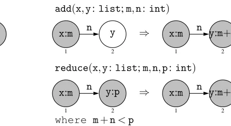
As a simple example, consider the program in Figure1for calculating shortest distances. The program expects input graphs with non-negative integers as edge labels, and arbitrary lists as node labels. There must be a unique marked node (drawn shaded) whose shortest distance to each reachable node has to be calculated. The rule schemata initand addappend distances

main=init;{add,reduce}!

init(x:list) add(x,y:list;m,n:int)

x

1

⇒ _x:0

1

x:m y

1 2

n _⇒

x:m y:m+n

1 2

n

reduce(x,y:list;m,n,p:int) x:m y:p

1 2

n

⇒ x:m y:m+n

1 2

n

where m+n<p

Figure 1: A program calculating shortest distances

to the labels of nodes that have not been visited before, whilereducedecreases the distance of nodes that can be reached by a path that is shorter than the current distance.

To construct the conflicts of the rule schemata add and reduce, their left-hand sides are overlayed. For example, the structure of the left-hand graph ofreducecan match the following structure in two different ways:

Consider a copy ofreducein which the variables have been renamed tox′,m′, etc. To match

reduceand its copy differently requires solving the system of equations hx:m=?_y′_:p′_,y:p=?

x′:m′i. Solutions to these equations should be as general as possible to represent all potential conflicts resulting from the above overlay. In this simple example, it is clear that the substitution

σ_={x′_7→y,m′_7→p,y′_7→x,p′_7→m}

x:p+n′ y:p

1 2

n

n′

⇐ x:m y:p

1 2

n

n′

⇒ x:m y:m+n

1 2

n

n′

In general though, equations can arise that have several independent solutions. For example, the equationhn:x=?_{y:2i(withnof typeintandx,yof typelist) has the minimal solutions}

σ_{1={x,y7→empty,n7→2} and} σ_{2={x7→z:2,y7→n:z}} whereemptyrepresents the empty list andzis a list variable.

Seen algebraically, we need to solve equations modulo the associativity and unit laws AU={x:(y:z) = (x:y):z,empty:x=x,x:empty=x}.

This problem is similar toword unification[BS01], which attempts to solve equations modulo associativity. (Some authors considerAU-unification as word unification, e.g. [Jaf90]). Solv-ability of word unification is decidable, albeit in PSPACE [Pla99], but there is not always a finite complete set of solutions. The same holds for AU-unification (see Section 3). Fortunately, GP’s syntax for left-hand sides of rule schemata forbids labels with more than one list variable. It turns out that by additionally forbidding shared list variables between different left-hand labels of a rule, rule overlays induce equation systems possessing finite complete sets of solutions.

This paper is the first step towards a static confluence analysis for GP programs. In Section3, we present a rule-based unification algorithm for equations between left-hand expressions of rule schemata. We show that the algorithm always terminates and that it is sound in that each substitution generated by the algorithm is an AU-unifier of the input equation. Moreover, the algorithm is complete in that every unifier of the input equation is an instance of some unifier in the computed set of solutions.

2

GP Rule Schemata

We refer to [Plu12,BFPR15] for the definition of GP and more example programs. In this sec-tion, we define (unconditional) rule schemata which are the “building blocks” of graph programs. Agraphover a label setC _{is a systemG= (V,E,s,t,l,m), whereV and E are finite sets of} nodes(orvertices) andedges,s,t:E→V are thesourceandtargetfunctions for edges,l:V→C is the node labelling function andm:E→C _{is the edge labelling function. We write}G₍C_)for the class of all graphs overC_.

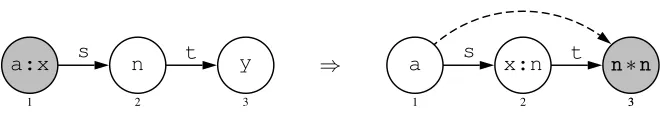
Figure2shows an example for the declaration of a rule schema. The typesintandstring

represent integers and character strings. Typeatomis the union ofintandstring, andlist

represents lists of atoms. Given listsl1 andl2, we writel1:l2for the concatenation ofl1andl2. The empty list is denoted byempty. In pictures of graphs, nodes or edges without label (such as the dashed edge in Figure2) are implicitly labelled with the empty list. We equate lists of length one with their entry to obtain the syntactic and semanticsubtyperelationships shown in Figure3. For example, all labels in Figure2are list expressions.

bridge(x,y:list;a:atom;n:int;s,t:string)

a:x

1

n

2

y

3

s t

⇒ a

1

x:n

2 3

n∗n

3

s t

Figure 2: Declaration of a GP rule schema

Figure4defines four syntactic categories of expressions: Integer, String, Atom and List, where Integer and String are subsets of Atom which in turn is a subset of List. Category Node is the set of node identifiers used in rule schemata. Moreover, IVar, SVar, AVar and LVar are the sets of variables of typeint,string,atomandlist. We assume that these sets are disjoint and define Var=IVar∪SVar∪AVar∪LVar. The mark components of labels are represented graphically rather than textually.

Each expression lhas a unique smallest type, denoted by type(l), which can be read off the

list

atom

int string

char

⊆

⊆ ⊇

⊆

(Z_∪Char∗₎∗

Z_∪Char∗ Z _Char∗

Char

⊆

⊆ ⊇

⊆

Figure 3: Subtype hierarchy for labels

Integer ::= Digit{Digit} |IVar

|‘−’ Integer|Integer ArithOp Integer |length‘(’ LVar|AVar|SVar ‘)’ |(indeg|outdeg) ‘(’ Node ‘)’ ArithOp ::= ‘+’|‘-’|‘∗’|‘/’

String ::= ‘ “ ’{Char}‘ ” ’|SVar|String ‘.’ String Atom ::= Integer|String|AVar

List ::= empty|Atom|LVar|List ‘:’ List Label ::= List [Mark]

Mark ::= red|green|blue|grey|dashed|any

hierarchy in Figure3afterlhas been normalised with the rewrite rules shown at the beginning of Subsection3.2. We write type(l1)<type(l2)or type(l1)≤type(l2)to compare types according to the subtype hierarchy. If the types ofl1andl2are incomparable, we write type(l1)ktype(l2).

The values of rule schema variables at execution time are determined by graph matching. To ensure that matches induce unique “actual parameters”, expressions in the left graph of a rule schema must have a simple shape.

Definition 1 (Simple expression) A simple expression contains no arithmetic operators, no length or degree operators, no string concatenation, and at most one occurrence of a list variable. In other words, simple expressions contain no unary or binary operators except list concatena-tion, and at most one occurrence of a list variable. For example, given the variable declarations of Figure2,a:xandy:n:nare simple expressions whereasn∗2orx:yare not simple.

Our definition of simple expressions is more restrictive than that in [Plu12] because we exclude string concatenation and the unary minus. These operations (especially string concatenation) would considerably inflate the unification algorithm and its completeness proof, without posing a substantial challenge.

Definition 2(Rule schema) Arule schema hL,R,Iiconsists of graphs L,RinG_{(Label) and} a set I, the interface, such that I =VL∩VR. All labels in L must be simple and all variables

occurring inRmust also occur inL.

When a rule schema is graphically declared, as in Figure 2, the interfaceI is represented by the node numbers inLandR. Nodes without numbers inLare to be deleted and nodes without numbers inRare to be created. All variables inRhave to occur inLso that for a given match of Lin a host graph, applying the rule schema produces a graph that is unique up to isomorphism.

Assumption 1(Left-linearity). We assume that rule schematahL,R,Iiareleft-linear, that is, the labels of different nodes or edges inLdo not contain the same list variable.

This assumption is necessary to ensure that the solutions of the equations resulting from over-laying two rule schemata can be represented by a finite set of unifiers. For example, without this assumption it is easy to construct two rule schemata that induce the system of equations hx:1=?_y,y=?_{1:xi. This system has solutions{x7→empty,y7→1},{x7→1,y7→1:1},}

{x7→1:1,y7→1:1:1}, . . . which form a infnite, minimal and compete set of solutions (See Definition5below).

3

Unification

3.1 Preliminaries

Asubstitutionis a family of mappingsσ_{= (}σ_X)

X∈{I,S,A,L}whereσI: IVar→Integer,σS: SVar→

String,σ_{A: AVar→Atom,}σ_{L: LVar→List. Here Integer, String, Atom and List are the sets of} expressions defined by the GP label grammar of Figure4. For example, ifz∈LVar,x∈IVar andy∈SVar, then we writeσ_{={x7→x+1,z7→y:−x:y}for the substitution that mapsxto}

x+1,ztoy:−x:yand every other variable to itself.

Applying a substitutionσ _{to an expression t, denoted byt}σ_{, means to replace every variable} xintbyσ_{(x)simultaneously. In the above example,(z:−x)}σ_{=y:−x:y:−(x+1).}

By Dom(σ_{)we denote the set{x∈Var|}σ_{(x)6=x}and by VRan(}σ_{)the set of variables} occur-ring in the expressions{σ_{(x)|x∈Var}. A substitution}σ_{isidempotentif Dom(}σ_)∩VRan(σ_{) = /0.} Thecompositionof two substitutionsσ_andθ_{, is defined asx(}σ_◦θ_{) =}

(

(xσ₎θ _ifx∈Dom(σ₎ xθ _otherwise and is an associative operation.

Definition 3(Unification problem) Aunification problemis a pair of an equation and a substi-tution

P=hs=?_t,σ

Pi

wheresandtare simple list expressions without common variables.

The symbol =? _{signifies that the equation must besolved rather than having to hold for all} values of variables. The purpose ofσ_{P is for the unification algorithm (Section3.2) to record a} partial solution. An illustration of this concept will be seen inFigure 8.

InSection 2, we already assumed that GP rule schemata need to be left-linear. Now, the prob-lem of solving a system of equations{s1=t1,s2=t2}can be broken down to solving individual equations and combining the answers - ifσ_{1 and} σ_{2 are solutions to each individual equation,} thenσ_1∪σ_{2is a solution to the combined problem as}σ_1andσ_{2do not share variables.}

Consider the equational axioms for associativity and unity, AU={x:(y:z) = (x:y):z,empty:x=x,x:empty=x}

wherex,y,zare variables of typelist, and let=AUbe the equivalence relation on expressions generated by these axioms.

Definition 4(Unifier) Given a unification problemP=hs=?_t,σ

PiaunifierofPa is a

substi-tutionθ _{such that}

sθ_=AUtθ _andxiθ_=AUtiθ for each binding{x_i7→t_i}inσ_{P .}

The set of all unifiers ofPis denoted byU_{(P). We say thatPisunifiableif}U_(P)6=/0. The special unification problem fail represents failure and has no unifiers. A problem P = hs=?_{t,∅iisinitialandP=h∅,σ}

A substitutionσ _{ismore generalon a set of variablesX than a substitution}θ _{if there exists a} substitutionλ _{such that x}θ _=AUxσ λ _{for all x∈X. In this case we write} σ_≦X θ _{and say that} θ _{is aninstanceof}σ _{onX. Substitutions}σ _andθ _{areequivalentonX, denoted by}σ _=X θ_{, if} σ_≦X θ_andθ_≦X σ_.

Definition 5(Complete set of unifiers [Plo72]) A setC _{of substitutions is acomplete set of} unifiersof a unification problemPif

1. (Soundness)C _⊆U_{(P), that is, each substitution in}C _{is a unifier ofP, and}

2. (Completeness) for eachθ_∈U_{(P)there exists}σ_∈C _{such that}σ_≦Xθ_{, whereX =Var(P)} is the set of variables occurring inP.

SetC _{is alsominimalif each pair of distinct unifiers in}C _{are incomparable with respect to}≦_X. If a unification problemPis not unifiable, then the empty set∅_{is a minimal complete set of} unifiers ofP.

For simplicity, we replace=?_{with=in unification problems from now on.}

Example1 The minimal complete set of unifiers of the problemha:x=y:2i(whereais an

atom variable andx,yare list variables) is{σ_1,σ_2}with

σ_{1={a7→2,x7→empty,y7→empty} and} σ_{2={x7→z:2,y7→a:z}.}

We have σ_{1(a:x) =2:empty=AU2=AUempty:2=}σ_{1(y:2) and} σ_{2(a:x) =a:z:2=} σ_{2(y:2). Other unifiers such as}σ_{3={x7→2,y7→a}are instances of}σ_2.

3.2 Unification Algorithm

We start with some notational conventions for the rest of this section: • L,Mstand for simple expressions,

• x,y,zstand for variables of any type (unless otherwise specified), • a,bstand for

(i) simple string or integer expressions, or (ii) string, integer or atom variables • s,tstand for

Preprocessing. Given a unification problemP=hs=?_{t,σi, we rewrite the terms in sand t} using the reduction rules

L:empty→L and empty:L→L

whereLranges over list expressions. These reduction rules are applied exhaustively before any of the transformation rules. For example,

x:empty:1:empty→x:1:empty→x:1.

We call this processnormalization. In addition, the rules are applied to each instance of a trans-formation rule (that is, once the formal parameters have been replaced with actual parameters) before it is applied, and also after each transformation rule application.

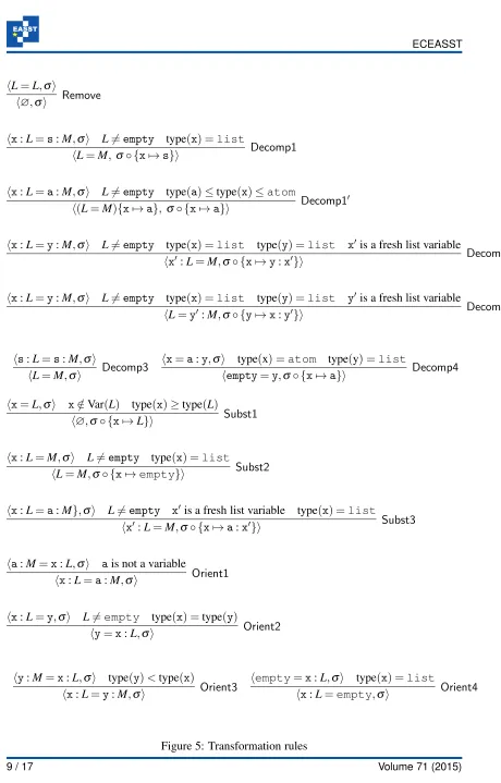
Transformation rules. Figure5shows the transformation rules, the essence of our approach, in an inference system style where each rule consists of a premise and a conclusion.

Remove: deletes trivial equations

Decomp1: syntactically equates a list variable with an atom expression or list variable

Decomp1’: syntactically equates an atom variable with an expression of lesser type

Decomp2/2’: assigns a list variable to start with another list variable Decomp3: removes identical symbols from the head

Decomp4: solves an atom variable Subst1: solves a variable

Subst2: assignsemptyto a list variable

Subst3: assigns an atom prefix to a list variable Orient1/2: moves variables to left-hand side

Orient3: moves variables of larger type to left-hand side Orient4: moves a list variable to the left-hand side

The rules induce a transformation relation⇒on unification problems. In order to apply any of the rules to a problemP, the problem part of its premise needs to bematchedontoP. Subse-quently, the boolean condition of the premise is checked and the ruleinstanceis normalized so that its premise is identical toP.

For example, the ruleOrient3can be matched toP=ha:2=m,σ_{i(whereaandmare variables} of typeatomandlist, respectively) by settingy7→a,x7→m,M7→2, andL7→empty. The rule instance and its normal form are then

ha: 2=m:empty,σ_i hm:empty=a: 2,σ_i and

ha: 2=m,σ_i hm=a: 2,σ_i

hL=L,σ_i

h∅,σ_i Remove

hx:L=s:M,σ_{i L6=empty type(x) =list}

hL=M,σ_{◦ {x7→s}i} Decomp1

hx:L=a:M,σ_{i L6=empty type(a)≤type(x)≤atom}

h(L=M){x7→a}, σ_{◦ {x7→a}i} Decomp1 ′

hx:L=y:M,σ_{i L=6 empty type(x) =list type(y) =list x}′_{is a fresh list variable}

hx′:L=M,σ_{◦ {x7→y:x}′_}i Decomp2

hx:L=y:M,σ_{i L=6 empty type(x) =list type(y) =list y}′_{is a fresh list variable}

hL=y′:M,σ_{◦ {y7→x:y}′_}i Decomp2 ′

hs:L=s:M,σ_i

hL=M,σ_i Decomp3

hx=a:y,σ_{i type(x) =atom type(y) =list}

hempty=y,σ_{◦ {x7→a}i} Decomp4

hx=L,σ_{i x∈/Var(L) type(x)≥type(L)}

h∅,σ_{◦ {x7→L}i} Subst1

hx:L=M,σ_{i L6=empty type(x) =list}

hL=M,σ_{◦ {x7→empty}i} Subst2

hx:L=a:M},σ_{i L6=empty x}′ _{is a fresh list variable type(x) =list}

hx′:L=M,σ_{◦ {x7→a:x}′_}i Subst3

ha:M=x:L,σ_{i ais not a variable}

hx:L=a:M,σ_i Orient1

hx:L=y,σ_{i L6=empty type(x) =type(y)}

hy=x:L,σ_i Orient2

hy:M=x:L,σ_{i type(y)<type(x)}

hx:L=y:M,σ_i Orient3

hempty=x:L,σ_{i type(x) =list}

hx:L=empty,σ_i Orient4

hx=L,σ_{i x∈Var(L) x6=L type(x) =list}

fail Occur

ha:L=empty,σ_i

fail Clash2

ha:L=b:M,σ_{i a6=b Var(a) = /0=Var(b)}

fail Clash1

hempty=a:L,σ_i

fail Clash3

hx=L,σ_{i type(x)ktype(L)}

fail Clash4

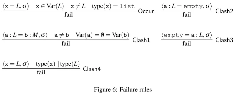
Figure 6: Failure rules

Showing that a unification problem has no solution can be a lengthy affair because we need to compute all normal forms with respect to⇒. Instead, the rulesOccurandClash1toClash4, shown inFigure 6, introducefailure. Failure cuts off parts of the search tree for a given problem P. This is because ifP⇒fail, thenPhas no unifiers and it is not necessary to compute another normal form. Effectively, the failure rules have precedence over the other rules. They are justified by the following lemmata.

Lemma 1 A normalised equationx=L withx6=L has no solution if L is a simple expression,

x∈Var(L)andtype(x) =list.

Proof. Sincex∈Var(L)andx6=L,Lis of the forms1:s2:. . .:snwithn≥2 andx∈Var(si)

for some 1≤i≤n. As L is normalised, none of the terms si contains the constant empty.

Also, sinceLis simple, it contains no list variables other thanxandxis not repeated. It follows σ_(x)6=AUσ_{(L)for every substitution}σ_.

Lemma 2 Equations of the forma:L=emptyorempty=a:L have no solution ifais an atom expression.

Lemma 3 An equationa:L=b:M witha6=bhas no solution ifaandbare atom expressions without variables.

The algorithm. The unification algorithm in Figure7starts by normalizing the input equation, as explained above. It uses a queue of unification problems to search the derivation tree of P with respect to⇒in a breadth-first manner. The first step is to put the normalized problemPon the queue.

The variable nextholds the head of the queue. If nextis in the formh∅,σ_{i, then} σ _{is a} unifier of the original problem and is added to the setUof solutions. Otherwise, the next step is to construct all problemsP′ such thatnext⇒P′. IfP′ isfail, then the derivation tree below

Unify(P): U:=/0

create empty queueQof unification problems normalizeP

Q.enqueue(hP,∅_i)

while Qis not empty

next:=Q.dequeue()

if nextis in the formh∅_,σ_i

U:=U∪ {σ_}

else ifnext;_fail

foreachP′ such thatnext⇒P′

normalizeP′ Q.enqueue(P′)

end foreach end if end if end while returnU

Figure 7: Unification algorithm

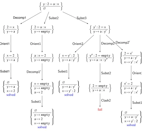
An example tree traversed by the algorithm is shown in Figure 8. Nodes are labelled with unification problems and edges represent applications of transformation rules. The root of the tree is the problemhy:2=a:xito which the rulesDecomp1,Subst2andSubst3can be applied. The three resulting problems form the second level of the search tree and are processed in turn. Eventually, the unifiers

σ_{1 = {x7→2,y7→a}} σ_{2 = {x7→y}′_:2,y7→a:y′_}

σ_{3 = {a7→2,x7→empty,y7→empty}}

are found, which represent a complete set of unifiers of the initial problem. Note that the set is not minimal becauseσ_{1is an instance of}σ_2.

The algorithm is similar to the A-unification (word unification) algorithm presented in [Sch92] which looks at the head of the problem equation. That algorithm terminates for the special case that the input problem has no repeated variables, and is sound and complete. Our approach can be seen as an extension from A-unification to AU-unification, to handle the unit equations, and presented in the rule-based style of [BS01]. In addition, our algorithm deals with GP’s subtype system.

3.3 Termination and Soundness

y: 2=a:x

∅

2=x y7→a

x=2

y7→a

 

 ∅

y7→a x7→2

   solved Subst1 Orient1 Decomp1

2=a:x y7→empty

a:x=2

y7→empty

 



x=empty

y7→empty

a7→2

          ∅

y7→empty

a7→2

x7→empty

       solved Subst1 Decomp1′ Orient1 Subst2

y′: 2=x y7→a:y′

x=y′: 2

y7→a:y′

 

 ∅

y7→a:y′ x7→y′: 2

   solved Subst1 Orient2

y′′: 2=empty

y7→a:x:y′′

2=empty

y7→a:x

fail Clash2 Subst2 Decomp2    2=x′ y7→a:y′ x7→y′:x′

     

x′=2

y7→a:y′ x7→y′:x′

      ∅

y7→a:y′ x7→y′:2

   solved Subst1 Orient1 Decomp2′ Subst3

Theorem 1 (Termination) If P is a unification problem without repeated list variables, then there is no infinite sequence P⇒P1⇒P2⇒. . .

Proof. Define thesize|L|of an expression Lby • 0 ifL=empty,

• 1 ifLis an expression of category Atom (see Figure4) or a list variable, • |M|+|N|+1 ifL=M:N.

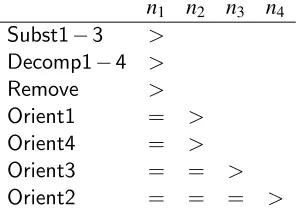
We define a lexicographic termination order by assigning to a unification problem P=hL= M,σ_{ithe tuple(n1,n2,n3,n4), where}

• n1is the size ofP, that is,n1=|L|+|M|;

• n2= (

0 ifLstarts with a variable 1 otherwise

• n3= (

1 if type(x)>type(y) 0 otherwise

wherexandyare the starting symbols ofLandM • n4=|L|

The table in Figure9shows that for each transformation stepP⇒P′, the tuple associated with P′ is strictly smaller than the tuple associated withPin the lexicographic order induced by the componentsn1ton4.

n1 n2 n3 n4

Subst1−3 >

Decomp1−4 >

Remove >

Orient1 = >

Orient4 = >

Orient3 = = >

Orient2 = = = >

Figure 9: Lexicographic termination order

Lemma 4 If P⇒P′, thenU_(P)⊇U_(P′_{) .}

Proof. We show that for each transformation rule, a unifier θ _{of the conclusion unifies the}

premise.

Note that forRemove, Decomp3andOrient1-4, we have thatσ_P′ =σ_P .

• Remove

θ_∈U_(h∅_,σ_P′i) ⇐⇒ θ∈U(h∅,σ_Pi)

⇐⇒ θ_∈U_(h∅_,σ_Pi)∧Lθ_=Lθ ⇐⇒ θ_∈U_(hL=L,σ_Pi)

• Decomp3

θ_∈U_(hL=M,σ_P′i) ⇐⇒ θ∈U(hL=M,σ_Pi)

⇐⇒ θ_∈U_(hL=M,σ_Pi)∧sθ_=sθ ⇐⇒ θ_∈U_(hs:L=s:M,σ_Pi) • Decomp1- We havexθ_=sθ _andLθ_=Mθ_.

Then(x:L)θ_{= (s:L)}θ_{= (s:M)}θ _{as required.} • Decomp1’- We havexθ_=aθ _andLθ_=Mθ_.

Then(x:L)θ_{= (a:L)}θ_{= (a:M)}θ _{as required.} • Decomp2- We havexθ_{= (y:x}′₎θ _and(x′_:L)θ_=Mθ_.

Then(x:L)θ_{= (y:x}′_:L)θ_{= (y:M)}θ_{as required.} • Decomp2’- We haveyθ_{= (x:y}′₎θ _andLθ_{= (y}′_:M)θ_.

Then(y:M)θ_{= (x:y}′_:M)θ_{= (x:L)}θ_{as required.} • Decomp4- We havexθ_=aθ _andyθ_{= (empty)}θ_=empty.

Then(a:y)θ_{= (x:y)}θ_{= (x:empty)}θ_=xθ_{as required.} • Subst1- We havexθ_=Lθ

θ_∈U_(h∅_,σ_S′i) ⇐⇒ θ∈U(h∅,σ_S◦(x7→L)i)

⇐⇒ θ_∈U_(h∅_,σ_{S◦(x7→L)i)∧x}θ_=Lθ ⇐⇒ θ_∈U_(hx=L,σ_Si)

• Subst2- We havexθ_{= (empty)}θ_andLθ_=Mθ_. Then(x:L)θ_{= (empty:L)}θ_=Lθ_=Mθ_{as required.} • Subst3- We havexθ_{= (a:x}′₎θ _and(x′_:L)θ _=Mθ_.

Then(x:L)θ_{= (a:x}′_:L)θ_{= (a:M)}θ_{as required.}

Theorem 2(Soundness) If P⇒+P′with P′=h∅_,σ_P′iin solved form, thenσ_P′ is a unifier of

P.

Proof. We have thatσ_P′ is a unifier ofP′by definition. A simple induction withLemma 4shows

thatσ_P′ must be a unifier ofP.

3.4 Completeness

In order to prove that our algorithm is complete, byDefinition 5we have to show that for any unifierδ_{, there is a unifier in our solution set that is more general.}

Our proof involves using aselectoralgorithm that takes a unification problemhs=?_titogether with an arbitrary unifier δ_{, and outputs apath of the unification tree associated with a more} general unifier than δ_{. This is very similar to [Sie78] where completeness of a A-unification} algorithm is shown via such selector.

Due to space restrictions the following lemma is given without proof. For the selector algo-rithm and proof (comprising of an extra 9 pages) see the long version of this paper [HP14]. Lemma 5(Selector Lemma) There exists an algorithmSelect(δ_,s=?_{t)that takes an equation} s=?_{t and a unifierδ as input and produces a sequence ofselectionsB = (b}

1, . . . ,bk)such that:

• Unify(s=?_{t) has a path specified by B .}

• For all selections b∈B: if σ _{is the substitution corresponding to b, then there exists an} instantiationλ _{such that}σ_◦λ_≤δ _.

For example, consider the unification problem hy:2=a:xi and δ _{= (x7→1:2,y7→a:1)} as a unifier. The unification tree was shown inFigure 8. Select(δ_{,y:2=a:x) would produce} selections(Subst3, Decomp2’, Orient1, Subst1), which corresponds to the right-most path in the tree. The unifier at the end of this path isσ _{= (x7→y}′_:2,y7→a:y′_{) which is more general} thanδ _{by instantiation}λ_{= (y}′_7→1).

Now we are able to state our completeness result, which follows directly from Lemma5. Theorem 3(Completeness) For every unifierδ _{of a unification problemhs=}?_{ti, there exist a} unifierσ_{generated byUnifysuch that}σ_≤δ _.

4

Conclusion

Future work includes establishing a Critical Pair Lemma in the sense of [Plu05]; this entails developing a notion ofindependent rule schema applications, as well as restriction and embed-ding theorems for derivations with rule schemata. Another topic is to consider critical pairs of conditional rule schemata (see [EGH+12]).

In addition, since critical pairs contain graphs labelled with expressions, checking joinability of critical pairs will require sufficient conditions under which equivalence of expressions can be decided. This is because the theory of GP’s label algebra includes the undecidable theory of Peano arithmetic.

Acknowledgements: We thank the anonymous referees of GCM 2014 for their comments on previous versions of this paper.

Bibliography

[BFPR15] C. Bak, G. Faulkner, D. Plump, C. Runciman. A Reference Interpreter for the Graph Programming Language GP 2. InProc. Graphs as Models (GaM 2015). Electronic Proceedings in Theoretical Computer Science 181, pp. 48–64. 2015.

[BS01] F. Baader, W. Snyder. Unification Theory. In Robinson and Voronkov (eds.), Hand-book of Automated Reasoning. Pp. 445–532. Elsevier and MIT Press, 2001.

[EEPT06] H. Ehrig, K. Ehrig, U. Prange, G. Taentzer.Fundamentals of Algebraic Graph Trans-formation. Monographs in Theoretical Computer Science. Springer-Verlag, 2006.

[EGH+12] H. Ehrig, U. Golas, A. Habel, L. Lambers, F. Orejas. M-Adhesive Transformation Systems with Nested Application Conditions. Part 2: Embedding, Critical Pairs and Local Confluence.Fundamenta Informaticae118(1):35–63, 2012.

[GLEO12] U. Golas, L. Lambers, H. Ehrig, F. Orejas. Attributed Graph Transformation with Inheritance: Efficient Conflict Detection and Local Confluence Analysis Using Ab-stract Critical Pairs.Theoretical Computer Science424:46–68, 2012.

[HKT02] R. Heckel, J. M. K ¨uster, G. Taentzer. Confluence of Typed Attributed Graph Trans-formation Systems. In Proc. International Conference on Graph Transformation (ICGT 2002). Lecture Notes in Computer Science 2505, pp. 161–176. Springer-Verlag, 2002.

[HP14] I. Hristakiev, D. Plump. A Unification Algorithm for GP (Long version).

http://www.cs.york.ac.uk/plasma/publications/pdf/HristakievPlump.Full.GCM14.pdf, 2014.

[Pla99] W. Plandowski. Satisfiability of Word Equations with Constants is in PSPACE. In Symposium on Foundations of Computer Science (FOCS 1999). Pp. 495–500. IEEE Computer Society, 1999.

[Plo72] G. Plotkin. Building-in Equational Theories.Machine intelligence7(4):73–90, 1972. [Plu05] D. Plump. Confluence of Graph Transformation Revisited. In Middeldorp et al. (eds.), Processes, Terms and Cycles: Steps on the Road to Infinity: Essays Dedi-cated to Jan Willem Klop on the Occasion of His 60th Birthday. Lecture Notes in Computer Science 3838, pp. 280–308. Springer-Verlag, 2005.

[Plu12] D. Plump. The Design of GP 2. In Proc. International Workshop on Reduction Strategies in Rewriting and Programming (WRS 2011). Electronic Proceedings in Theoretical Computer Science 82, pp. 1–16. 2012.

[Sch92] K. U. Schulz. Makanin’s Algorithm for Word Equations: Two Improvements and a Generalization. InProc. Word Equations and Related Topics (IWWERT ’90). Lecture Notes in Computer Science 572, pp. 85–150. Springer-Verlag, 1992.