A Stochastic Restricted Maximum Likelihood Method for Genomic Selection and Genome-Wide Association Studies

(1)

UC Riverside

UC Riverside Electronic Theses and Dissertations

Title

Permalink

https://escholarship.org/uc/item/34q919vf

Author

Lin, Chen

Publication Date

2019 Peer reviewed|Thesis/dissertation

(2)

UNIVERSITY OF CALIFORNIA RIVERSIDE

A Dissertation submitted in partial satisfaction of the requirements for the degree of

Doctor of Philosophy in Applied Statistics by Chen Lin March 2019 Dissertation Committee:

Dr. Shizhong Xu, Chairperson Dr. Weixin Yao

(3)

Copyright by Chen Lin

(4)

The Dissertation of Chen Lin is approved:

Committee Chairperson

(5)

Acknowledgments

My most sincere thanks to my advisor, Dr. Shizhong Xu, for guiding and en-couraging me through my Ph.D experience. His creativity and enthusiasm for researches have been fundamentally influenced me, which will guide me profoundly. I also want to express my gratitude towards my co-advisor Dr. Weixin Yao and my committee member Dr. Zhenyu Jia for their support and valuable suggestions. I would like to thank all the fac-ulty and staff in the department for their help. I am grateful to my lab members, Ruidong Li, Han Qu, Meiyue Wang, Shibo Wang, Fangjie Xie, Tiantian Zhu for their support and friendship. I am extremely thankful to my friends Hua Peng, Lijie Li for their companion-ship. I would also like to thank all my other friends who have supported me along the way. Lastly, I sincerely thank my parents for their unconditional love and encouragement.

(6)

(7)

ABSTRACT OF THE DISSERTATION

by Chen Lin

Doctor of Philosophy, Graduate Program in Applied Statistics University of California, Riverside, March 2019

Dr. Shizhong Xu, Chairperson

Genomic selection is a marker-assisted methodology that dramatically decreases the cost of measuring phenotypes by using the whole-genome information to predict and select de-sirable individuals. In plant breeding, it plays an important role to speed up the breeding cycles. Modern techniques make obtaining marker information from the entire genome feasible. However, it results in high dimensionality of predictors when we implement a mathematical model to estimate the parameters and predict future crosses. Many statis-tical models including variable selection models can address this problem and have been applied in genomic selection. Variable selection models can also be applied in GWAS which is a powerful tool to discover the association between genetic variation and variation in quantitative traits.

A novel statistical approach based on BLUP was proposed to be implemented in both genomic selection and GWAS. The general idea of the proposed approach is using an algorithm to divide markers into the small effect group and the large effect group. Markers within the large effect group can be potentially significant markers associated with the

(8)

analyzed phenotypic trait. In Chapter 3, we used simulated data and two real-world data sets to demonstrate the distinctions among six statistical methods for genomic selection. In addition, the proposed model was applied in GWAS based on another simulated data, and the proposed model is superior to the other two variable selection models.

(9)

List of Figures

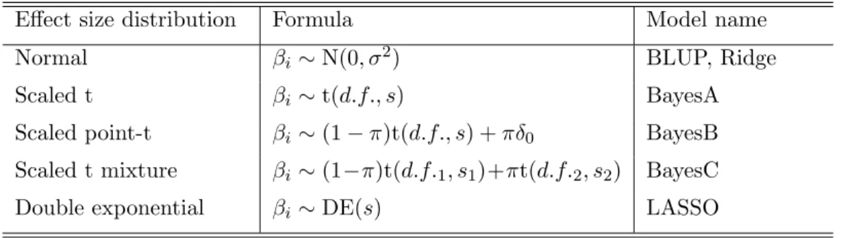
2.1 Prior densities of marker effects. Top left panel is a normal prior. Top right panel is thick-tail priors. Bottom right panel is a scaled t mixture prior. Bottom left panel is a scaled point-t panel. . . 24 3.1 Left panel is the density plot of Beta distribution with a=5,000 and b=500.

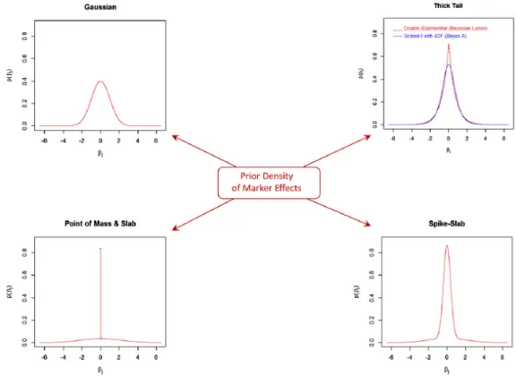
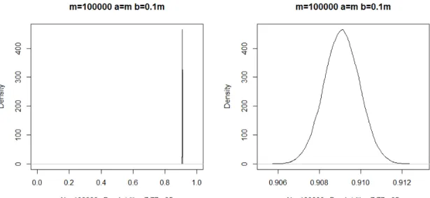
Right panel enlarges the peak part of the left panel. . . 35 3.2 Left panel is the density plot of Beta distribution with a=100,000 and b=10,000.

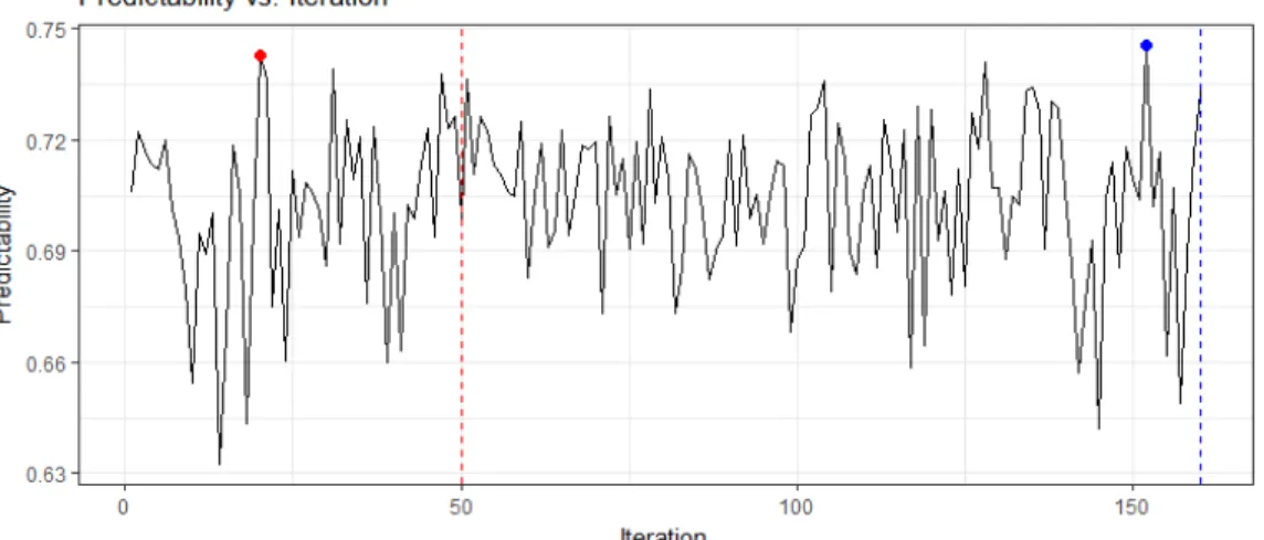
Right panel enlarges the peak part of the left panel. . . 35 3.3 Predictability of a trait plotted against the iteration numbers. The red dash

line represents the iteration number is 50, and the blue dash line represents the iteration number is 160. Two solid points are the corresponding iteration numbers with highest predictabilities. . . 36 3.4 This is an example to depict 5-fold CV. A data set is divided into 5 folds and

each fold will be our testing data. . . 38 3.5 The true large marker effects and the estimated large marker effects under

six methods in Scenario II. . . 42 3.6 The true small marker effects and the estimated small marker effects under

six methods in Scenario II. . . 43 3.7 Simulated QTL effects and their marker positions. Upper plot exhibits all

21 markers and their genetic effects. Lower plot exhibits 19 highly correlated markers and their genetic effects. . . 47 3.8 Comparison of FDR and FNR among SREML, LASSO, and BayesB in

Scenario I. SREML XXX1, SREML XXX2, SREML XXX3 represent the thresholds used for SREML in this simulation study were 0.5, 0.45, and 0.4, respectively. The threshold for BayesB was 0.2. The number of replicates per σ2 was 250. . . 50

(12)

3.9 Comparison of FDR and FNR among SREML, LASSO, and BayesB in Scenario II. SREML XXX1, SREML XXX2, SREML XXX3 represent the thresholds used for SREML in this simulation study were 0.5, 0.45, and 0.4, respectively. The threshold for BayesB was 0.3. The number of replicates per σ2 was 250. . . 50 3.10 Comparison of probabilities among SREML, LASSO, and BayesB in Scenario

I. SREML1, SREML2, SREML3 represent the thresholds used for SREML in this simulation study were 0.5, 0.45, and 0.4, respectively. The threshold for BayesB was 0.2. The number of replicates per σ2 was 250. . . 53 3.11 Comparison of probabilities among SREML, LASSO, and BayesB in Scenario

II. SREML1, SREML2, SREML3 represent the thresholds used for SREML in this simulation study were 0.5, 0.45, and 0.4, respectively. The threshold for BayesB was 0.3. The number of replicates per σ2 was 250. . . 54

(13)

List of Tables

2.1 Effect size (βi) distributions, their formulas and model names. sdenotes the

scale parameter. d.f. denotes the degrees of freedom parameter. δ0 denotes

a point mass at zero. π denotes a high probability value. . . 23 3.1 Comparison of the predictability for simulated data under six methods. All

predictabilities were calculated by squared correlation between predicted re-sponse variable and observed rere-sponse variable. These averaged results were drawn from ten different 10-fold CVs to reduce the partitioning variation. All methods were evaluated under the same fold IDs. The iteration num-ber of SREML was 50. Scenario I represents only one marker had a constant large effect (20), and remaining markers had small effects and were randomly sampled from normal distribution with mean 0 and variance 0.04. Scenario II represents 81 markers (5% of 1619 markers) had large effects and again remaining markers were drawn from variance 0.04. . . 41 3.2 The estimated large marker effects under six methods in Scenario I. . . 41 3.3 Comparison of the predictability for the IMF2 population under six methods.

All predictabilities were calculated by squared correlation between predicted response variable and observed response variable. The averaged results were drawn from ten different 10-fold CVs to reduce the partitioning variation for the IMF2 population. All methods were evaluated under the same fold IDs. The iteration number of SREML was 50. . . 44 3.4 Comparison of the predictability for the elite hybrid rice data under six

meth-ods. All predictabilities were calculated by squared correlation between pre-dicted response variable and observed response variable. The averaged results were drawn from a 5-fold CV. All methods were evaluated under the same fold IDs. The iteration number of SREML was 20. SubscriptHZ represents the hybrid varieties were planted in Hangzhou. SubscriptSY represents the hybrid varieties were planted in Sanya. . . 45 3.5 Comparison of the standard deviation for FDR under three models in

Sce-nario I. SREML1, SREML2, SREML3 represent the thresholds used for SREML were 0.5, 0.45, and 0.4, respectively. The threshold for BayesB was 0.2. The number of replicates per σ2 was 250. . . 51

(14)

3.6 Comparison of the standard deviation for FDR under three models in Sce-nario II. SREML1, SREML2, SREML3 represent the thresholds used for SREML were 0.5, 0.45, and 0.4, respectively. The threshold for BayesB was 0.3. The number of replicates perσ2 was 250. . . 51 3.7 Comparison of the standard deviation for FNR under three models in

Sce-nario I. SREML1, SREML2, SREML3 represent the thresholds used for SREML were 0.5, 0.45, and 0.4, respectively. The threshold for BayesB was 0.2. The number of replicates per σ2 was 250. . . 52 3.8 Comparison of the standard deviation for FNR under three models in

Sce-nario II. SREML1, SREML2, SREML3 represent the thresholds used for SREML were 0.5, 0.45, and 0.4, respectively. The threshold for BayesB was 0.3. The number of replicates perσ2 was 250. . . 52 3.9 Comparison of TNR and its standard deviation under three models in

Sce-nario II. SREML1, SREML2, SREML3 represent the thresholds used for SREML were 0.5, 0.45, and 0.4, respectively. The threshold for BayesB was 0.3. The number of replicates perσ2 was 250. . . 55 3.10 Variance components estimated by SREML and BLUP in Scenario II. . . . 65

(15)

Chapter 1

Introduction

1.1 Genomic Selection

A long time ago, people had to spend a lot of months or even years to obtain desirable animals or plants. Since 1990s, marker-assisted selection (MAS) has been used to indirectly select desirable candidates with the genetic markers significantly associated with a particular trait. However, this methodology is time-consuming attributed to the long breeding cycles and genetic information loss. In contrast, genomic selection provides a way to overcome these limitations. It is well-known as a marker-assisted methodology that drastically reduces the cost of measuring quantitative traits by using the whole-genome information to predict and directly select desirable individuals. Here selection stands for selecting future individuals based on the predicted phenotypes rather than selecting ge-netic markers associated with a quantitative trait. It is particularly useful to accelerate the breeding process. Moreover, it facilitates to predict phenotypic values for a breeding population (they are only genotyped) according to the model fitted in a training population

(16)

(they are both genotyped and phenotyped) (Desta and Ortiz, 2014). Genomic selection has been applied in many areas, such as human beings, as well as animal and plant species. In next subsection, we introduce the applications of genomic selection in these areas.

1.1.1 Applications of Genomic Selection

Genomic selection has been widely used since 2001. Meuwissen et al. (2001) at-tempted to use the whole genomic information to build the linear regression model and predict breeding values in a simulated data set based on animal genotypes under BLUP. They also proposed new methods (BayesA and BayesB) and compared the results drawn from new methods with BLUP. The limitations of genomic selection are the requirement of a large number of markers and the cost of marker discovery. Fortunately, these problems were addressed a few years later. Hayes et al. (2009) investigated and summarized the accuracy of genomic breeding values (GEBV) in Holstein-Friesian dairy cattle from Aus-tralia, New Zealand, and the United States (Harris et al., 2009; VanRaden et al., 2009). A total of 4,500 bulls and a total of 44,146 markers were involved in New Zealand dairy cattle analysis. A total of 730 bulls and a total of 38,259 markers were involved in Aus-tralia dairy cattle analysis. The application of dairy cattle in the United States consisted of a total of 3,576 bulls and a total of 38,416 markers. New Zealand and America dairy cattle populations achieved the similar accuracies, and Australia dairy cattle data had the lowest accuracy. Erbe et al. (2012) combined Holstein and Jersey reference populations to improve prediction accuracy in Jersey cattle. Besides dairy cattle, genomic selection was applied in other animal species as well. For instants, Legarra et al. (2008) examined three strategies of selection for four complex traits in a mouse population including 1,884 mice

(17)

and 10,946 markers. Lee et al. (2008) proposed a Bayesian method and implemented in a heterogeneous stock mouse population to predict unobserved phenotypic values.

Genomic selection has been applied in animal species for a long time. However, it is in its infancy in plant breeding and humans. Bernardo and Yu (2007) compared results drawn from genomic selection with results drawn from MAS under BLUP in a maize pop-ulation and concluded genomic selection outperformed MAS. Piepho (2009) investigated ridge regression and some other methods in maize. Heffner et al. (2009) summarized tech-nologies used in genomic selection for crop improvement. Xu et al. (2014) exploited hybrid prediction in genomic selection. A total of 278 hybrids was used to predict 21,945 poten-tial hybrids to select top crosses. Yang et al. (2010) uncovered the missing heritability for human height using whole-genome information.

1.2 Genome-wide Association Studies (GWAS)

In genetics, GWAS (Risch and Merikangas, 1996) is another crucial field. It facili-tates to discover genetic variation associated with a complex or quantitative trait (including diseases) in a genome-wide panel of markers. A linear mixed model is widely used to identify the statistical associations between single-nucleotide polymorphisms (SNPs) and phenotypic traits. It consists of covariate effects, a single marker fixed effect, polygenic effects controlled by all other genes, and it is well-known as single-SNP tests, i.e. testing one SNP at a time. GWAS provide a powerful tool to define phenotypic traits across individuals and disclose the causal relationship between genetic variants and phenotypic differences. Dis-covering the underlying genetic architecture provides insights into the understanding of

(18)

complex traits and disease susceptibility. It has been successfully applied in many areas, such as human diseases and economic traits in crops.

1.2.1 Applications of GWAS

Many human diseases have been investigated, and the associated SNPs have been uncovered. For coronary heart disease (CHD), Consortium et al. (2011) identified five new markers associated with CHD risk in Europeans and South Asians; Domarkien˙e et al. (2013) identified two important loci associated with CHD risk in Lithuanian Families. For type 2 diabetes mellitus (T2D), Sim et al. (2011) exploited significant loci associated with T2D in multi-ethnic cohorts including Chinese, Malays, and Asian Indians; Ghassibe-Sabbagh et al. (2014) identified two markers associated with T2D in the Lebanese population to verify the key role of these two loci in Southwest Asian populations. Li et al. (2015) analyzed 10 pediatric-age-of-onset autoimmune diseases (pAIDs) and revealed 27 significant markers related to one or more pAIDs. Michailidou et al. (2017) detected 65 new loci associated with breast cancer in a population including European ancestry and East Asian ancestry.

In crops, Huang et al. (2010) performed GWAS to investigate˜3.6 million loci across 517 diverse rice landraces for 14 agronomic traits including tiller number, grain weight, grain width, etc. They also proposed a novel data-imputation method to construct a high-density haplotype map. A total of 80 significant associations were detected for 14 agronomic traits. In 2011, 44,100 SNPs obtained from 413 diverse accessions of Oryza sativa were used to discover the relationships with 34 quantitative traits (Zhao et al., 2011). Dozens of common variants were identified to have influences on numerous traits. Jia et al. (2013) conducted GWAS of 47 agronomic traits based on˜2.58 million SNPs by sequencing 916 diverse foxtail

(19)

millet varieties. A total of 512 association signals had relationships with 47 agronomic traits. Chen et al. (2014) carried out GWAS to find the associations between genetic variants and metabolic traits by using˜6.4 million SNPs based on 529 diverseOryza sativaaccessions.

1.2.2 Single-SNP Tests

One of the most commonly used models in GWAS is linear mixed model (LMM) (Yu et al., 2006). The model for markerican be written as

y=Xβ+ziγi+ξ+e,

ξ∼MVNn(0, ZZTσξ2), e∼MVNn(0, Iσ2e)

wherey is ann×1 vector of phenotypic values,Xis a knownn×qdesign matrix associated

with fixed effects, β is aq×1 vector of unknown fixed effects, Z is a known n×m genetic

matrix,zi is theith column ofZ,γiis an unknown fixed effect associated with ith marker,ξ

is the polygenic effect,eis ann×1 vector of random errors andi= 1, . . . , m. MVN denotes

a multivariate normal distribution. Every marker in the data set is required to be scanned to estimate its fixed marker effect γi. Unknown parameters can be estimated using REML method (introduced in Chapter 2).

The purpose of GWAS is to reveal markers significantly associated with a complex trait. Based on LMM, a hypothesis testing can be conducted to test the significance of the

ith marker, i.e. H0 :γi = 0. The Wald test statistic for it is Wi =

ˆ

γ_i2

(20)

Under the null hypothesis, H0:γi = 0, the distribution ofWi isWi∼χ21. Then thep-value

of the markeriis

pi = 1−Pr(χ2₁≤Wi).

For a single hypothesis test, p-value is usually compared with the level of significance α, also known as the type I error. Ifp-value is less than or equal to α, then we reject the null hypothesis; otherwise, the null hypothesis is failed to be rejected. However, for multiple comparisons (testing multiple hypotheses simultaneously), if we keep using the same crite-rion, the overall type I error, family-wise error rate (FWER), will vastly increase. FWER can be defined by

FWER = Pr(V≥1),

where V is the number of false positives, i.e. how many true null hypotheses are rejected. If we assume hypotheses are independent of each other, then FWER can be calculated by FWER = 1−(1−α)m. Suppose m = 100 and α = 0.05, then FWER=0.99. It implies

any m exceeding 100 leads to 100% probability that at least one null hypothesis will be rejected incorrectly. In order to address it, it is necessary to correct the level of significance in multiple comparisons.

One of the simplest and most popular correction methods is Bonferroni correction. It simply adjusts the level of significance by α/m, where m is the number of hypotheses. According to Boole’s inequality, FWER has the property that it will be controlled within

αifpi ≤ _mα. Bonferroni correction assumes hypotheses are independent, but GWAS violate

this assumption because of correlations existing among markers. Due to it, Bonferroni correction is conservative and leads to statistical power reduction.

(21)

In contrast to single-SNP tests, polygenic modeling with variable selection fea-ture is an alternative way to identify important markers, such as LASSO, BayesB, etc. It estimates all marker coefficients simultaneously. Therefore, multiple comparisons are not involved in it. Here is an example of using LASSO in GWAS: Wu et al. (2009) implemented LASSO penalized logistic regression to identify important markers associated with coeliac diseases.

Details about polygenic modeling are introduced in Chapter 2.

1.3 The Stochastic EM Algorithm

In statistics, a lot of problems involves missing data or incomplete data. One of the most popular algorithms to solve these problems is the Expectation-Maximization (EM) algorithm (Dempster et al., 1977). The main idea of the EM algorithm is replacing maximization of the log likelihood function of the observed data with maximization of the conditional expectation of unobserved data.

Let us define the complete data as x= (y, z) and it can be sampled from f(x|θ),

where y denotes the observed data, z denotes the unobserved data or the latent variables, and θ denotes the unknown parameters. It’s difficult to compute the likelihood function of the observed data, f(y|θ) = R_zf(y, z|θ)dz, in many situations. Then the conditional

expectation of unobserved data z given the observed data y and the estimated parameters

θ(t) is used and it is written as

Q(θ|θ(t)) = E_z_|_y,θ(t)(L(θ;y, z)),

(22)

The EM algorithm generates estimates as follows:

Step 1 (E step): Compute the conditional expectation of z,Q(θ|θ(t)).

Step 2 (M step): Estimate unknown parameters θ(t+1) by maximizingQ(θ|θ(t)). However, the EM algorithm is difficult to implement in some cases. Stochastic EM algorithms provide powerful tools to deal with the cases that can not be handled by the EM algorithm, including the SEM algorithm (Celeux, 1985), MCEM (Wei and Tanner, 1990), etc. In order to converge the estimates quickly, a stochastic EM algorithm is drawing the unobserved samples from the conditional density, f(z|y, θ). After that, the likelihood

function can be directly maximized. This idea is implemented in our proposed method introduced in Chapter 3.

(23)

Chapter 2

Statistical Models Overview

With the remarkable advances in computing technology, millions of single-nucleotide polymorphisms (SNPs), a common type of genetic variation, can be obtained using mod-ern genome sequencing technologies. Namely, high-density markers are involved in recent researches. In quantitative genetics, we treat SNPs or markers as our predictors and vari-ation in quantitative traits of individuals as our response variable. The goals of statistical models are to find the relationship between our predictors and the response variable, and to estimate all coefficients simultaneously.

High-density marker panels provide more genetic information to improve the pre-dictive accuracy. On the other hand, it also leads to the number of predictors substantially exceeding the number of individuals in a statistical model, and multicollinearity of predic-tors, i.e. high intercorrelations existing among several independent predictors. In ordinary least squares (OLS) regression, high dimensionality of markers results in a singular matrix which implies the solution is not unique, and multicollinearity causes the reduction of the statistical power. Fortunately, many other polygenic methodologies can deal with these

(24)

issues in statistics. In general, there are two types of these methodologies: linear regression models and nonlinear regression models. Specifically, we focus on linear models because of interpretability. Linear models dealing with high dimensionality issue mainly include regularized linear regression models, the linear mixed model, and Bayesian approaches.

2.1 Regularized Linear Regression Models

To solve high dimensionality problem of predictors, regularized linear regression models add a penalty term into the sum of squared residuals, i.e. penalized residual sum of squares, and then minimize it to estimate the unknown parameters. The general model can be written as follows

y=µ+Xβ+e, e∼MVNn(0, Iσe2),

where y is ann×1 vector of a response variable measured on n individuals, µis an n×1

vector of intercept terms, X is an n×m design matrix (m > n), β is an m×1 vector

of unknown parameters, e is an n×1 vector of random errors, and MVNn represents the

n-dimensional multivariate normal distribution.

If y and X are both centered, denoted by ˜y and ˜X,then the unknown parameter

β can be estimated with the following equation ˆ β = arg min β n X i=1 (˜yi−x˜Ti β)2+λf(β),

where ˜xT_i is theithrow of ˜X,λ≥0 is a shrinkage factor which controls the size of coefficients.

The larger value of λ, the smaller value of β. f(·) represents the penalized function of β.

(25)

to ridge regression if the penalized function isl2 penalty term, i.e. f(β) =kβk22=

Pm i=1βi2

(Hoerl and Kennard, 1970a,b); a famous regularized regression model, the least absolute shrinkage selection operator (LASSO), is proposed if the penalized function is identical to

l1 penalty term, i.e. f(β) =kβk1=Pmi=1|βi|(Tibshirani, 1996).

There are two distinctions between two models. First, ridge regression shrinks all coefficients with equal sizes, while LASSO regression combines coefficient shrinkage and variable selection. l1-norm has an additional property of shrinking some coefficients towards

zero than l2-norm. Second, ridge regression has an analytical solution, but LASSO

regres-sion does not, which implies that ridge regresregres-sion is more statistically and computationally efficient than LASSO. Researchers have to develop faster algorithms to estimate LASSO pa-rameters. Efron et al. (2004) developed least angle regression (LARS) algorithm to reduce runtime complexity of the algorithm toO(nm2) which is the same as OLS. LARS algorithm played a crucial role to calculation LASSO estimation before 2010. Friedman et al. (2010) introduced a simpler and more flexible algorithm, known as pathwise coordinate descent, to reduce the computational cost toO(2nm). And this algorithm has still been widely used until now.

2.2 Linear Mixed Models

Another approach dealing with high dimensionality of predictors is linear mixed models, which is well-known as BLUP method. A linear mixed model can be expressed as

y =µ+Xβ+Zγ+e,

(26)

e∼MVNn(0, R),

whereyis ann×1 observation vector,µis ann×1 vector of intercept terms,X is a known

n×q matrix associated with fixed effects, β is a q×1 vector of unknown fixed effects, Z

is a known n×mmatrix associated with random effects, γ is anm×1 vector of unknown

random effects, andeis ann×1 vector of random errors. Note thatGandRare covariance

matrices ofγ and e, respectively. Then the variance ofy is

Var(y) =V =ZGZT +R.

If we assume covariance matrices G and R are known, Henderson (1963) showed that the best linear unbiased estimator (BLUE) of β is

ˆ

β = (XTV−1X)−1XTV−1y, (2.2.1)

and the best linear unbiased predictor (BLUP) of γ is

ˆ

γ =GZTV−1(y−Xβˆ). (2.2.2)

Both two equations depend upon the inverse ofV. If the number of observations is large, then the calculation of V−1 is computationally intensive. Henderson (1950) offered an alternative way to jointly obtain ˆβ and ˆγ using his mixed-model equations (MME),

    XTR−1X XTR−1Z ZTR−1X ZTR−1Z+G−1     ×     ˆ β ˆ γ     =     XTR−1y ZTR−1y     .

It has been proved that the solutions for ˆβ and ˆγ from MME are the BLUE and the BLUP, respectively (Henderson, 1963; Henderson et al., 1959).

BLUE and BLUP are based on known covariance matrices. However, in realistic cases, they are usually unknown. A popular method to estimate variance components ofG

(27)

and R is called the restricted maximum likelihood (REML) method, and the logarithm of the REML function is given by

L(θ) =−1 2lnV − 1 2 ln|X T_V−1_X_{| −} 1 2(y−X ˆ β)TV−1(y−Xβˆ),

whereθ consists of unknown variance components, and

ˆ

β = (XTV−1X)−1XTV−1y. 2.2.1 HAT Method

In order to select the best model among several models, the prediction errors are utilized to measure and compare the performance. Supposen1 independent individuals

(x1, y1), . . . ,(xn1, yn1) are the training data and the regression function fitted by the training

data is denoted by ˆfn1(·). Then the resulting models can be applied to predict the response

variable or phenotypic measurements at the testing dataxn1+1, . . . , xn1+n2. Usually, we use

the mean square prediction error (MSPE) to measure the accuracy of prediction. And it can be obtained by 1 n2 n2 X i=1 |yn1+i−fnˆ1(xn1+i)| 2_.

If data only consists ofnindependent observations, using the same data to fit and calculate MSPE generally leads to bad estimate of the prediction error, i.e. the prediction error is much lower than the true prediction error. One popular method to eliminate overfitting phenomenon is the cross-validation (CV) analysis. The general idea of k-fold CV (Picard and Cook, 1984) is that we partition the n observations into k equal-sized parts, where k≤ n. k−1 parts is considered as our training data and the remaining one

(28)

estimate the prediction errors. The overall prediction error is averaged acrosskMSPEs. A special case, known as the leave-one-out cross-validation (LOOCV), occurs withk =n. It was developed by Allen (1971, 1974) to calculate the predicted residual error sum of squares (PRESS), which is the average of n MSPEs drawn from the LOOCV analysis. Moreover, PRESS was proposed to use as a criterion to select the best model among several regression models.

Relative to PRESS, the predictability of a model is used to measure the per-formance as well. It can be expressed by the squared correlation coefficient between the observed and predicted phenotypic values (Xu et al., 2014). And it is also equal to

R2= 1−PRESS/SS,

where the value of PRESS is explained above and the SS is the total sum of squares of the response variable, i.e.

SS = 1 n n X i=1 (yi−y¯)2.

One limitation ofk-fold CV analysis is the random partitioning variation problems. To get rid of it, LOOCV is preferred to compute the prediction errors or predictabilities. However, LOOCV analysis will be computationally expensive when the sample size n is large. Therefore, HAT method was proposed to estimate the prediction errors in order to reduce the computational burden. In general, HAT method is a method to evaluate the prediction errors using the whole sample only once. Cook (1977, 1979) derived the formula to calculate PRESS for OLS by adjusting the coefficients of the linear regression model using the leverage values of observations (the diagonal elements of HAT matrix

(29)

effects model by finding the optimal shrinkage factor in ridge regression. Four decades later, Gianola and Sch¨on (2016) summarized how to implement the HAT method to compute the prediction errors by running the model only once. This paper derived the HAT methods for linear regression, ridge regression, Bayesian alphabet models, etc. In addition, for the ridge regression, it was claimed that using the shrinkage factor λ estimated by the whole sample instead of using the value estimated within each fold doesn’t affect the prediction errors too much, especially for the LOOCV analysis. Xu (2017) subsequently investigated the difference between them, and he provided the derivation of calculation of the LOOCV predictability for a mixed model as well. Here are the details about using HAT method under linear mixed model to obtain the predictability.

Recall a linear mixed model can be written as

y =Xβ+Zγ+e, (2.2.3)

γ ∼MVNm(0, Iσ2γ), e∼MVNn(0, Iσe2).

Let us define the predicted random effects as

ˆ

r= ˆy−Xβ,ˆ (2.2.4)

and the observed random effects as

r=y−Xβ,ˆ

where

ˆ

(30)

Substituting (2.2.1) and (2.2.2) into (2.2.4), we have

ˆ

r=σ_γ2ZZTV−1r=Hr,

whereH is called the HAT matrix. The estimated error vector is

ˆ

e=y−yˆ=r−rˆ=r−Hr= (I−H)r.

The predicted error for the ith observation is

ei=yi−xTi βˆ[−i]= (1−hii)−1ˆei,

where ˆβ[−i] is the estimate of β with the ith observation deleted and hii is the ith diagonal

element of the HAT matrix, called the leverage value of observation i. Then the PRESS is

PRESS = n X i=1 e2_i = n X i=1 (1−hii)−2eˆ2i.

Accordingly, the predictability of the model is

R2 = 1−PRESS SS where SS = n X i=1 (ri−¯r)2

is the total sum of squares of y after correction for the fixed effects.

2.3 Bayesian Alphabet Models

Apart from regularized linear regression models and linear mixed models, Bayesian approaches can also be used in genomic selection and GWAS. The key features of Bayesian approaches compared with previous models are Bayesian approaches incorporate another

(31)

information into the models and consider uncertainty of unknown parameters (Zhou et al., 2013). Frequentist inference usually treats model parameters as fixed values, while Bayesian inference treats them as random variables and assigns informative prior beliefs (prior distri-butions) to them. Then the posterior distributions of unknown parameters can be obtained using Bayes’ theorem. Moreover, the posterior distributions describe uncertainty in pa-rameter estimates. In genomic selection and GWAS, Bayesian alphabet models, BayeA, BayesB, and BayesC, are widely used (Meuwissen et al., 2001; Verbyla et al., 2009). The main differences among them are different model assumptions.

2.3.1 BayesA

Linear mixed models assume marker effect sizes come from normal distributions with homogeneous variances if the covariance matrixR=Iσ_γ2. It is not realistic to assume all effect sizes have equal variances. If the variances are varied from marker to marker, then BayeA is derived. The model can be showed in the expression below

y=µ+Xβ+e,

e|σ2_e ∼MVNn(0, Iσe2), βi|σ_i2 ∼N(0, σ_i2),

vector of intercept terms, X is an n×m design matrix, β is an m×1 vector of unknown

effect sizes, e is an n×1 vector of random errors, MVNn represents the n-dimensional

(32)

Suppose the prior distributions of σ2_e and σ2_i are

σ_e2 ∼χ−2(−2,0),

and

σ2_i ∼χ−2(ν, τ2),

where ν is the number of degrees of freedom and τ2 is a scale parameter. Since a scaled inverted chi-square distribution is a conjugate prior, the posterior distributions of σ2_e and

σ_i2 can be easily obtained and given by

σ_e2|e∼χ−2(n−2, eTe),

and

σ_i2|βi∼χ−2(ν+ 1, τ2+βi2).

Then the Gibbs sampling algorithm can be applied to estimate effect sizes and variances.

2.3.2 BayesB

BayesB assumes that a large number of markers have no genetic variances and a small number of markers have genetic variances. The model can be expressed by

y=µ+Xβ+e,

e|σ2_e ∼MVNn(0, Iσe2), βi|σ_i2 ∼N(0, σ_i2),

(33)

effect sizes, e is an n×1 vector of random errors, MVNn represents the n-dimensional

multivariate normal distribution, and i= 1, . . . , m.

Similarly, the prior distribution of σ_e2 is still the scaled inverted chi-square distri-bution with parameters {−2,0}. But forσ_i2, it is modified by

σ2_i ∼χ−2(ν, τ2) with probability 1−π, σ_i2 = 0 with probabilityπ,

where ν is the number of degrees of freedom, τ2 is a scale parameter, and π denotes a high density which reflects the proportion of markers without genetic effects. The posterior distributions of σ_e2 and σ2_i remain the scaled inverted chi-squared distributions. However, the Gibbs sampler of BayesA can not be implemented to sample the values of σ2_i and βi

here because samplingσ2_i = 0 is impossible whenβ_i2 6= 0. Thus, we need to take advantage of the joint distribution of σ_i2 and βi given y∗, i.e.

p(σ2_i, βi|y∗) =p(βi|σi2, y∗)×p(σi2|y∗),

wherey∗ is the response variable y corrected for the overall mean andβ_[−i] (genetic effects

withoutβi). Thenσi2can be sampled fromp(σi2|y∗) andβican be sampled fromp(βi|σi2, y∗).

This algorithm is computationally intensive because the Metropolis-Hasting (MH) algorithm is implemented to sample the values fromp(σ2

i|y∗). Cheng et al. (2015) introduced

three different Gibbs samplers to sample the parameters without the MH algorithm. They enhance the running speed twice faster than the Gibbs sampler with the MH algorithm.

(34)

2.3.3 BayesC

Since original BayesB is computationally expensive, Verbyla et al. (2009) proposed and suggested a new Bayesian method, which is known as method BayesC. Then model can be described as

y=µ+Xβ+e, e|σ2_e ∼MVNn(0, Iσe2),

βi|ui, σi2∼uiN(0, σ2i/100) + (1−ui)N(0, σi2),

vector of intercept terms, X is an n×m design matrix, β is an m×1 vector of unknown

effect sizes,eis ann×1 vector of random errors,uiis a binary indicator variable for theith

marker (ui={0,1}), MVNn represents the n-dimensional multivariate normal distribution,

and i= 1, . . . , m.

The prior distributions of σ2_i and ui are σ2_i ∼χ−2(ν, τ2),

and

ui∼Bernoulli(πi),

where ν is the number of degrees of freedom, τ2 is a scale parameter and πi denotes a

high density. Based on the hierarchical prior assumptions, marker effects can be sampled from a mixture of the scaled t distributions. The indicator variable ui is sampled from the

posterior distributionp(ui = 1|βj, σi2, u[−i], y), i.e.

Bernoulli( p(βj|u[−i], ui = 1)(1−πi)

p(βj|u[−i], ui = 1)(1−πi) +p(βj|u[−i], ui= 0)πi

(35)

whereu[−i] is all the indicator variables with ui deleted.

2.4 Predictions

Supposen1 independent individuals (x1, y11), . . . ,(xn1, y1n1) are the training data

and n2 independent individuals xn1+1, . . . , xn1+n2 are the testing data. In this section, let

us discuss how we can calculate the predictions of a quantitative trait based on the model fitted in the training data, which is denoted by ˆfn1(·). According to previous sections, we

know that the basic models for regularized linear regression models and Bayesian alphabet models are the same, i.e.

y=µ+Xβ+e.

The differences among them are effect size assumptions and parameter estimates. Therefore, for these two types of models, the predictions at the testing data, ˆy2, can be easily calculated

by

ˆ

y2 = ˆfn1(X2) = ˆµ+X2β,ˆ

whereX2 = (xn1+1, . . . , xn1+n2)

T_.

However, the predictions in the linear mixed model is not straightforward. Here are the details. Recall the linear mixed model can be formulated as equation (2.2.3). Define the kinship matrix asK =ZZT_{. Then the extended kinship matrix is}

    K11 K12 K21 K22,     .

HereK11is then1×n1 kinship matrix with respect to the training observations,K22is the

(36)

matrix with respect to current crosses and future crosses. Then the predicted breeding values ofy2 is ˆ y2 =X2βˆ+σγ2K21V₁−1(y1−X1βˆ), where ˆ β = (X₁TV₁−1X1)−1X1TV −1 1 y1, V1 =σγ2K11+Iσe2,

X1 is an n1×q design matrix, X2 is an n2×q design matrix, and y1 is an n1×1 vector

associated with current quantitative traits.

2.5 Summaries

All the models I discussed above belong to polygenic modeling, which is regressing genotypic values on a quantitative trait and estimating genetic effect sizes simultaneously. Table 2.1 lists the summaries of effect size distributions that have been developed to deal with high dimensionality of predictors. Regularized linear model estimates are equivalent to Bayesian estimates when regression coefficients are assigned appropriate priors. For instants, Bayesian estimates are identical to LASSO estimates when σi is assigned a prior distribution, an exponential prior. Then the marginal prior distribution of βi is double

exponential. Ridge regression is identical to BLUP if we define the shrinkage factor is the variance ratio in (2.2.3), i.e. λ=σ_e2/σ_γ2. One thing may be confused about table 2.1 is effect size distributions for Bayesian alphabet models. According to model assumptions, effect size distributions of Bayesian alphabet models are related to normal distributions. Since the prior distribution of genetic variance, σ_i2, is the scaled inverted chi-square distribution, the

(37)

marginal prior of βi results in the scaled t distribution. That is the reason that prior

distributions of Bayesian alphabet models are associated with the scaled t distributions. Different distributions of effect sizes lead to different model behaviors. Figure 2.1 (de los Campos et al., 2013) illustrates distributions of effect sizes listed in table 2.1. Relative to normal priors, scaled t and double exponential are known as thick-tail priors. A thick-tail prior or a scaled t mixture prior has a property that it tends to strongly shrink small effect sizes to zero and lightly shrink large effect sizes compared with a normal prior. The scaled point-t distribution makes variable selection feasible because of a point mass at zero with a high density.

Table 2.1 Effect size (βi) distributions, their formulas and model names. sdenotes the scale

parameter. d.f. denotes the degrees of freedom parameter. δ0 denotes a point mass at zero.

π denotes a high probability value.

Effect size distribution Formula Model name

Normal βi ∼N(0, σ2) BLUP, Ridge

Scaled t βi ∼t(d.f., s) BayesA

Scaled point-t βi ∼(1−π)t(d.f., s) +πδ0 BayesB

Scaled t mixture βi ∼(1−π)t(d.f.1, s1)+πt(d.f.2, s2) BayesC

(38)

Figure 2.1 Prior densities of marker effects. Top left panel is a normal prior. Top right panel is thick-tail priors. Bottom right panel is a scaled t mixture prior. Bottom left panel is a scaled point-t panel.

(39)

Chapter 3

A Stochastic Restricted Maximum

Likelihood Method

3.1 Introduction

In the past, plant breeders had to spend a lot of years to obtain desirable hy-brid crosses by planting various hyhy-brid rice varieties. Recently a new approach has been developed to accelerate the breeding process, i.e. genomic selection. Genomic selection is a methodology that provides desirable candidates with a shorter breeding cycle using millions of molecular markers information to predict future individuals. Therefore, the pre-dicted phenotypic values evaluated by the statistical models can easily detect the desirable individuals to reduce the cost of traditional breeding. This methodology has been used in many areas, such as humans, animals, and plants, however, it started to be applied in the hybrid prediction after 2014 (Xu et al., 2014).

(40)

Genomic selection is a marker-assisted selection method and numerous single-nucleotide polymorphisms (SNPs) are involved in it, therefore, it is important to implement the efficient and effective models to accurately predict phenotypic traits. Modern techniques facilitate the utilization of complicated linear or nonlinear statistical models for the pheno-typic predictions. Even through nonlinear models can achieve higher accuracy sometimes, linear models are easy to interpret and make marker selection feasible. Due to it, this dis-sertation only focuses on the linear models. The multiple linear regression model is one of the simplest and basic linear models. However, in plant breeding it is hard to implement it because of high dimensionality and multicollinearity of markers (Crossa et al., 2017). High dimensionality of markers means the number of markers substantially exceeds the number of individuals, which leads to nonexistence of design matrix inverses. And multicollinearity of markers results in the wrong signs and insignificance of coefficients. In order to address those problems, regularized linear regression models, such as ridge regression (Hoerl and Kennard, 1970a,b) and least absolute shrinkage selection operator (LASSO) regression (Tibshirani, 1996), the linear mixed model (Henderson, 1975), and Bayesian alphabet models, such as BayesA, BayesB and BayesC approaches (Meuwissen et al., 2001; Verbyla et al., 2009), have been proposed and widely used. Regularized linear models estimate unknown parameters by minimizing the least square and penalty terms. The regression coefficients influenced by different penalty terms are distinguishing, where shrinkage of estimates or variable selec-tion or even both can be achieved. For example, ridge regression uses l2 penalty term to

shrink coefficients while LASSO regression uses l1 penalty term to shrink coefficients and

select variables. In contrast, the linear mixed model, also known as the best linear unbiased prediction (BLUP) model, assigns a prior distribution with homogeneous variances to all

(41)

markers instead of adding penalty terms into the loss function. If heterogeneous variances are adopted across all markers, i.e. each marker has an unequal effect on phenotypic values, and each variance is assigned a prior distribution, then method BayesA is applied. Relative to method BayesA, if only a small number of markers have heterogeneous variances and remaining markers have null effects on the quantitative trait values, then method BayesB is adopted. Based on the definition of method BayesB, it is obvious that it makes marker selection feasible. If we assign ignorable values of variance to the remaining markers instead of treating them as zero, then method BayesC is derived.

Apart from genomic selection, in genetics, a genome-wide association study (GWAS) (Risch and Merikangas, 1996) is another crucial field, which is a study of exploiting the asso-ciations between some specific SNPs and valuable phenotypic traits using the entire genome information. For example, in plant breeding, we can detect which SNPs have sizable effects on an important trait, such as yield or grain. One of the most popular methods proposed to detect significant markers is linear mixed model (LMM) (Yu et al., 2006). However, this method is computationally costly because of large and many matrix multiplications and inverses. In order to speed up the running time, several algorithms have been developed, such as efficient mixed-model association (EMMA) (Kang et al., 2008), genome-wide effi-cient mixed-model association (GEMMA) (Zhou and Stephens, 2012), etc. The methods listed above test a single marker at a time, which means all markers need to be scanned to identify the relationships with the quantitative trait. One limitation of these approaches is the multiple testing problem, that is if a high-density SNP array is employed, then the level of significance should be extremely stringent. Further, the single-SNP approaches may not detect any single significant marker if markers are highly correlated to each other. In

(42)

terms of these two limitations, the methods estimating marker coefficients simultaneously outperform the single-SNP approaches. Among the methods I introduced above, LASSO and BayesB belongs to variable selection methods, or known as selective shrinkage methods, which can be used in GWAS as well. It is very convenient to use both models in R. LASSO can be easily implemented using GlmNet/R program (Friedman et al., 2010), and BayesB can be easily implemented using BGLR/R program (P´erez and de Los Campos, 2014). As mentioned earlier, LASSO uses l1 penalty term to shrink the coefficients of some markers

to exactly zero, but BayesB assumes the variance of each marker is zero with a known high probability or is a nonzero value with a low probability. Theoretically, BayesB can delete markers with zero variance.

It has been showed that BLUP is more robust than LASSO and BayesB under some conditions (Xu et al., 2014), and that is the motivation of proposing a new approach based on BLUP in genomic selection and GWAS. The contribution of the study is taking into account of the idea of a stochastic EM algorithm and a small group of markers with additional variances which facilitates to select variables. The general idea of the proposed approach is dividing markers into two classes, i.e. the large effect class and the small effect class. More details of it are described in the next section.

3.2 Materials and Methods

3.2.1 A Stochastic Restricted Maximum Likelihood Model

This approach consists of the REML step and the stochastic step. In the REML step, variance components can be estimated given the cluster labels of markers. In the

(43)

stochastic step, the cluster labels of markers are updated given variance components. The details of this approach are described as follows.

Consider mloci that are divided into mS loci with small effects andmL loci with large effects where mS+mL = m. Then define the indicator variable or cluster label of locusi by ui=       

0 if markeribelongs to the large effect cluster 1 if marker ibelongs to the small effect cluster

where ui ∼ Bernoulli(π) is a Bernoulli variable with a predetermined high probability

π = 0.95. This prior distribution assumes that 95% of the loci have small effects on the phenotypic values and the remaining 5% markers have sizable effects. It is possible to assign a conjugate prior, a Beta distribution, toπ so that the value ofπ can be updated using the data information, but for simplicity of the method we set a constant value for this parameter at first.

A linear mixed model with two random components can be formulated as

y=Xβ+ZSγS+ZLγL+e, (3.2.1) γS ∼MVNmS(0, Iσ 2 S), γL∼MVNmL(0, Iσ 2 L), e∼MVNn(0, Iσe2).

Here yis ann×1 observation vector,X is ann×q covariate matrix including an intercept

vector,βrepresents aq×1 non-genetic fixed effect vector,ZSandZLaren×mS small effect

marker andn×mL large effect marker matrices,γS and γLare mS×1 andmL×1 genetic

(44)

an n×1 vector of error terms. Note that MVNarepresents thea-dimensional multivariate

normal distribution, and σ_S2 < σ2_L. Define Z as the whole marker matrix and Zi as the

numerical coded values of theith marker for all individuals. Then the two polygenic vector

which are random effect can be written as

ZSγS = m X i=1 uiZiγi, and ZLγL= m X i=1 (1−ui)Ziγi,

whereγi is the effect of theith locus and is treated as a random effect with mean zero and

variance

Var(γi) =uiσ2_S+ (1−ui)σ2_L,

which implies the variance of γi is equal to σS2 if the ith locus belongs to the small effect

cluster andσ_L2 if the ith locus belongs to the large effect cluster. Then the expectation ofy

is

E(y) =Xβ,

and the varianceV is

Var(y) =ZSVar(γS)ZST +ZLVar(γL)ZLT + Var(e)

=KSσS2 +KLσL2 +Iσe2.

Here KS=ZSZST andKL=ZLZLT are called kinship matrices.

Given ui, the unknown parameters θ = {σS2, σ2L, σ2e} can be estimated using the

restricted maximum likelihood (REML) method. After the unknown parameters are es-timated, the new labels for each locus can be updated. Bayes’ theorem is applied to

(45)

sample a new u(_it+1) conditional on the current value u(_it) and all other parameter val-ues. Given the current valueu(_it) and θ(t), the conditional posterior probability of u(_it+1) is

P(u(_it+1)= 1|u_i(t), θ(t)) =ρi, and ρi is expressed as

ρi=

π

π+ (1−π)exp(ψ),

where

ψ= (1−2u(_it))[L(θ(t))−Li(θ(t))],

and L(θ) is the restricted log likelihood function without changing the labels, andLi(θ) is the restricted log likelihood function when theith_{marker switches its current cluster label,}

i.e., from the small effect cluster to the large effect cluster or vice versa, depending on its current position. Therefore, the conditional posterior distribution of ui can be obtained according to Bernoulli(ρi) and a new u(it+1) is sampled based on it.

To switch the cluster label for marker i, we need to update the kinship matrices. If theith marker is currently in the small effect cluster, a switch will place this marker to

the large effect cluster and the new variance matrix will be

V+i =V −ZiZiTσS2 +ZiZiTσL2.

A switch from the large effect cluster to the small effect cluster will result in a new variance matrix of

V−i =V −ZiZiTσL2 +ZiZiTσS2.

Since the current cluster label for marker i is u(_it), if u(_it) = 1, the ith marker is currently in the small effect cluster and a switch means placing it to the large effect cluster and thus we should take V+i. Similarly, if u(_it) = 0, we should switch marker i from the large effect

(46)

cluster to the small effect cluster and thusV−i should be taken. Incorporating u(it) into the

establishment of the new variance matrix, we have

Vi =V −(1−2u(_it))(ZiZ_iTσ_L2 −ZiZ_iTσ2_S) =V −(1−2u(_it))(σ2_L−σ2_S)ZiZiT

=V −(1−2u_i(t))∆ZiZiT,

where ∆ = σ_L2 −σ2_S is the difference between the large variance and the small variance. Then the restricted log likelihood function of switching markeriis

Li(θ) =− 1 2ln|Vi| − 1 2ln|X T_V−1 i X| − 1 2(y−Xβˆ) T_V−1 i (y−Xβˆ) where ˆ β = (XTV_i−1X)−1XTV_i−1y.

Looping over all markers represents an extremely large computational burden due to calculations ofV_i−1and|Vi|. However, we can avoid it by taking advantage of Woodbury matrix identities for the inverse and the matrix determinant lemma for the determinant, which are

V_i−1 = [V −(1−2u_i(t))∆ZiZiT]−1

=V−1−V−1Zi[ZiTV−1Zi−(1−2u(it))∆

−1_]−1_ZT i V−1

for the inverse and

|Vi|=|V −(1−2u(it))∆ZiZiT|

(47)

for the determinant. Therefore, the obvious advantage computationally is that we do not need to calculate the marker specific matrix inverse and determinant anew but simply update from V−1 and |V|. Looking back at the likelihood function, we notice that V_i−1

never occurs alone but always exists in a quadratic form like aTV_i−1b, where a and b can be X, Zi, y ory−Xβˆ. These quadratic forms are expressed by

aTV_i−1b=aTV−1b−aTV−1Zi[ZiTV−1Zi−(1−2u(it))∆

−1_]−1_ZT i V−1b.

Tremendous computational time can be saved via this special algorithm.

The proposed method involves stochastic sampling for the cluster labels of mark-ers given the variance component parametmark-ers and REML estimation of variance parametmark-ers given the cluster labels of markers. Iterations are required over the stochastic step and the REML step, and thus the method is called stochastic restricted maximum likelihood (SREML) method. During the SREML process, for each iteration the predictability is evalu-ated using the HAT method (Xu, 2017), where the leave-one-out cross validation (LOOCV) mean squared prediction error (MSPE) can be obtained by fitting the data values only once. Then the maximum predictability and the corresponding u vector will be recorded. The number of iterations is quite arbitrary but does not need to be very large. If 20 consecutive iterations fail to identify better performance, we may stop the SREML process and report the predictability and its associated u vector. The longer the iterations, the higher the chance to identify the best classification.

An enhancement of the SREML is to estimate π from the data rather than to fix its value at 0.95. Suppose we assign a conjugate prior to π, Bata(a, b). Then the posterior distribution remains Beta, i.e. Bata(a+mS, b+mL), where mS =

Pm

(48)

mL = Pmi=1(1−ui). One of the reasonable choices of a and b is a = m and b = 0.1m.

Figure 3.1 and figure 3.2 illustrate Beta distributions whenm=5,000 andm=100,000. The comparison of two figures tell us no matter the value of m is small or large, a random variable sampled from a Beta distribution will be approximately equal to 0.91. It implies we expect a large number of loci to be small effect cluster. From the posterior distribution, Bata(a+mS, b+mL), a new π is sampled. π(t+1) is then used to update the uvector.

Figure 3.3 is an example of the SREML procedure when we adopt the HAT method as our criterion and it shows the predictability against the iteration number. The red and blue dashed lines represent the iteration number is 50 and 160 respectively; the red and blue dots represent the maximum predictability locations for different iteration numbers. This figure illustrates that the procedure of the SREML randomly goes up and down, and we have more chance to obtain a better result as the iteration number increases. We also can conclude that the process is stochastically around an invisibly horizontal line and the best predictability will be found during the process.

(49)

Figure 3.1 Left panel is the density plot of Beta distribution with a=5,000 and b=500. Right panel enlarges the peak part of the left panel.

Figure 3.2 Left panel is the density plot of Beta distribution with a=100,000 and b=10,000. Right panel enlarges the peak part of the left panel.

(50)

Figure 3.3 Predictability of a trait plotted against the iteration numbers. The red dash line represents the iteration number is 50, and the blue dash line represents the iteration number is 160. Two solid points are the corresponding iteration numbers with highest predictabilities.

3.2.2 Algorithm

Start at t= 0 with a randomly initiated value u(0)_i ,i= 1,2, ..., mand π(0)= 0.95. Givenu(0)_i and π(0), the algorithm generates estimates as follows:

Step 1 (REML step): Estimate variance components{σ_S2, σ_L2, σ_e2}by the restricted log likelihood function given the current estimates {u(_it), π(t)}.

Step 2 (Stochastic step): Update the cluster label u(_it+1) and π(t+1) given the estimated variance components {σ_S2, σ_L2, σ_e2}.

Step 3: Iterate between step 1 and step 2 until the maximum number of iterations has been reached.

Step 4: Select the estimates of the variance components and theuvector associated with the maximum predictability.

(51)

3.3 Results

3.3.1 Genomic Selection

Some statistical values, such as MSE, are commonly computed to compare the performance among prediction models. However, it will cause overly optimistic estimates of prediction error if the training data set is used to fit models and calculate prediction errors simultaneously. Therefore, cross-validation (CV) method is widely used to compare statistical models for eliminating overfitting phenomenon(Meuwissen et al., 2001). The general idea of k-fold CV (Picard and Cook, 1984) is to partition n observations into k

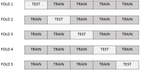
approximately equal-sized parts. Observations of k-1 folds are considered as the training data to build prediction models and the remaining fold is the testing data set to estimate the prediction errors. This process will be repeatedktimes such that every fold will be the testing data set, and the overall prediction error is the average of k testing MSEs. Figure 3.4 is an example of 5-fold CV. A data set is divided into 5 folds and each fold will be our testing data.

Moreover, to straightforwardly compare the results among different models and different data types, the predictability, which is approximately equal to squared correlation between predicted response variable and observed response variable (Xu et al., 2016), will be the criterion in this section, where the range is from 0 to 1.

The sources of the data sets applied in this study are publicly available and have been published online. And they can be obtained from the literatures cited.

(52)

Figure 3.4 This is an example to depict 5-fold CV. A data set is divided into 5 folds and each fold will be our testing data.

3.3.1.1 A Simulation Study

A simulation study was performed to demonstrate the comparison of the pre-dictability under six methods, which are SREML, BLUP, LASSO, BayesA, BayesB, and BayesC. LASSO results were obtained via GlmNet in R package. And Bayesian alphabet models implemented BGLR in R package with the number of iterations=3,500 and the num-ber of burn-in=500. The real 1,619 genetic markers were used to generate 278 observations (More details about these real genetic markers are described in real-world data analysis). And simulated datay was generated using the model 3.2.1, whereq = 1 and the fixed effect term only contained the intercept term µ, whose value was fixed to a constant value 100. There were two scenarios in this simulation study: in Scenario I, only one genetic marker was randomly selected with large genetic effect (γL = 20), the remaining genetic effects were sampled from N(0, Iσ2_S) and the error term was sampled from N(0, Iσ2_e); in Scenario

(53)

II, 5% of 1,619 genetic markers were randomly selected and their effects were sampled from N(0, Iσ_L2), the remaining genetic effects were sampled from N(0, Iσ2_S) and the error term was sampled from N(0, Iσ2_e). The average value of ten 10-fold CV results was calculated to measure the predictive performance sincek-fold CV would lead to the random partitioning variation problem. Note that large effect marker positions were consistent in ten 10-fold CVs for either scenario.

In Chapter 2, I introduce the formulas to calculate the predictive breeding values of BLUP method for a breeding population (testing data). But it only works for BLUP with one random component. Here let us discuss the prediction of BLUP with two random components first. Define the dimension of observed individuals as n1, the dimension of

future individuals as n2, and the dimension of genetic markers for one individual as m.

Then the extended kinship matrices can be expressed as

    KS11 KS12 KS21 KS22,     , and     KL11 KL12 KL21 KL22,     .

HereKS11is an n1×n1 kinship matrix with respect to the training observations measured

on small effect markers, KL11 is an n1 ×n1 kinship matrix with respect to the training

observations measured on large effect markers, KS22 is an n2 ×n2 kinship matrix with

respect to future crosses measured on small effect markers, KL22 is an n2 ×n2 kinship

matrix with respect to future crosses measured on large effect markers, and (KS12, KS21)

(54)

measured on small effect markers and large effect markers, respectively. Note that we don’t need to calculate all components for prediction, and we only need KS11, KL11, KS21 and

KL21. Then the predicted breeding values ofy2 is

ˆ y2=X2βˆ+ (σS2KS21+σL2KL21)V₁−1(y1−X1βˆ), where ˆ β = (X₁TV₁−1X1)−1X1TV −1 1 y1, V1=σS2KS11+σL2KL11+Iσ2e,

X1 is an n1×q design matrix, X2 is an n2×q design matrix, and y1 is an n1×1 vector

associated with current phenotypic values.

As mentioned earlier, the predictability is measured using corr2(y2,yˆ2), where corr

denotes the correlation coefficient. If we setσ2_S= 0.04,σ_L2 = 400,σ_e2 = 1, the initial value of

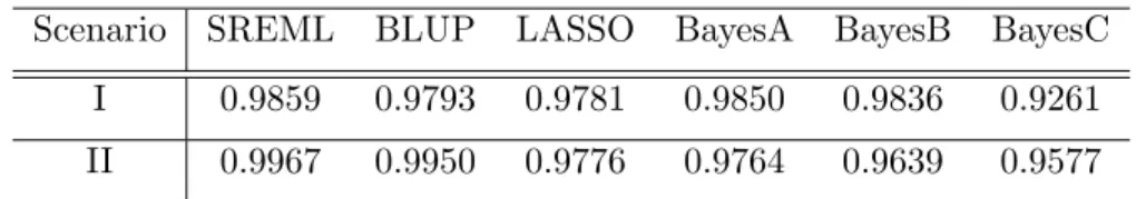
π is 0.95 and the iteration number of SREML is 50, then the predictabilities are displayed in table 3.1. All methods produces similar results for both scenarios. Among these six methods, SREML slightly outperforms other methods. BayesC has the worst results, the predictabilities are 0.9261 and 0.9577 for Scenario I and II.

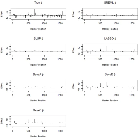
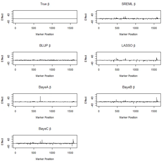
Table 3.2 lists the estimated large marker effect under six methods in Scenario I. The parameters were estimated by the whole sample. It shows BLUP heavily shrinks the coefficients to zero. Estimates from LASSO, BayesA, BayesB are close to the true value of marker effects. Figure 3.5 illustrates true large marker effects and the estimated marker effects under six models in Scenario II. Figure 3.6 illustrates true small marker effects and

(55)

Table 3.1 Comparison of the predictability for simulated data under six methods. All predictabilities were calculated by squared correlation between predicted response variable and observed response variable. These averaged results were drawn from ten different 10-fold CVs to reduce the partitioning variation. All methods were evaluated under the same fold IDs. The iteration number of SREML was 50. Scenario I represents only one marker had a constant large effect (20), and remaining markers had small effects and were randomly sampled from normal distribution with mean 0 and variance 0.04. Scenario II represents 81 markers (5% of 1619 markers) had large effects and again remaining markers were drawn from variance 0.04.

Scenario SREML BLUP LASSO BayesA BayesB BayesC

I 0.9859 0.9793 0.9781 0.9850 0.9836 0.9261

II 0.9967 0.9950 0.9776 0.9764 0.9639 0.9577

Table 3.2 The estimated large marker effects under six methods in Scenario I. Marker βtrue βSREM L βBLU P βLASSO βBayesA βBayesB βBayesC

502 20 7.56 1.94 17.59 20.61 20.56 8.47

the estimated marker effects under six models in Scenario II. Variance components estimated by SREML and BLUP in Scenario II are listed in Appendix 3.B.

3.3.1.2 Real-world Data Analysis

The IMF2 population (Xu et al., 2016), i.e. the immortalized F2 population,

was used to demonstrate the comparison of predictabilities under six methods applied in the simulation study. A total of 278 crosses were generated by randomly pairing the 210 recombinant inbred lines (RILs), and a total of 1,619 bins inferred from 270,820 SNPs were treated as the genetic markers (Yu et al., 2011). Four traits were analyzed to examine the prediction accuracy, which were tiller number per plant (TILLER), grain number per plant

(56)

Figure 3.5 The true large marker effects and the estimated large marker effects under six methods in Scenario II.

(57)

Figure 3.6 The true small marker effects and the estimated small marker effects under six methods in Scenario II.

(58)

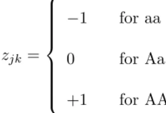
(GRAIN), yield (YIELD), and 1000-grain weight (KGW), respectively. The numerical value for thekth marker in the jth cross was coded as

zjk =                −1 for aa 0 for Aa +1 for AA

where aa, Aa and AA were three genotypes of a single marker. Four traits showed in Table 3.3 are predictabilities drawn from ten 10-fold CVs with six methods for this data set. The iteration number of SREML was 50. Compared with the simulation study, SREML results lose its edge. Table 3.3 implies SREML has similar results with other methods, and there is not a unique method outperforming the remaining methods. The model performance depends on the traits we analyzed.

Table 3.3 Comparison of the predictability for the IMF2 population under six methods. All predictabilities were calculated by squared correlation between predicted response variable and observed response variable. The averaged results were drawn from ten different 10-fold CVs to reduce the partitioning variation for the IMF2 population. All methods were evaluated under the same fold IDs. The iteration number of SREML was 50.

Trait SREML BLUP LASSO BayesA BayesB BayesC

TILLER 0.2194 0.2374 0.1960 0.2470 0.2452 0.2464

GRAIN 0.3607 0.3659 0.3680 0.3776 0.3826 0.3688

YIELD 0.1411 0.1314 0.1537 0.1401 0.1449 0.1387

KGW 0.6871 0.6958 0.6968 0.7001 0.7045 0.6934

The other data used to compare the prediction accuracy among six method was from 1,495 elite hybrid rice varieties (Huang et al., 2015). A total of 38 agronomic traits were investigated, and the hybrid varieties were planted at two locations, Sanya and Hangzhou in China. The genotypes of the rice hybrids consisted of totally 182,010 SNPs and the

(59)

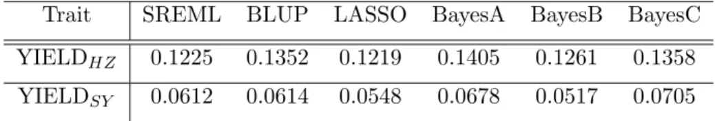
numerical coded value for each marker was the same as the IMF2 population. Several quantitative traits were contained in this data set, such as YIELD, disease-resistance traits, etc. Because YIELD is a very important trait for the hybrid rice and it relates to global food supply which needs to satisfy the increasing human demanding, the YIELDs at two different locations were selected to be analyzed. Table 3.4 indicates the predictabilities among six methods for YIELDs planted in Hangzhou and Sanya. Due to the high quantity of genetic markers, a 5-fold CV was used to evaluate the predictabilities, and the iteration number of SREML was 20. As with the IMF2 data set, the performance of SREML in table 3.4 is moderate, and Bayesian alphabet models barely outperform other models.

Table 3.4 Comparison of the predictability for the elite hybrid rice data under six methods. All predictabilities were calculated by squared correlation between predicted response vari-able and observed response varivari-able. The averaged results were drawn from a 5-fold CV. All methods were evaluated under the same fold IDs. The iteration number of SREML was 20. SubscriptHZ represents the hybrid varieties were planted in Hangzhou. SubscriptSY

represents the hybrid varieties were planted in Sanya.

Trait SREML BLUP LASSO BayesA BayesB BayesC

YIELDHZ 0.1225 0.1352 0.1219 0.1405 0.1261 0.1358

YIELDSY 0.0612 0.0614 0.0548 0.0678 0.0517 0.0705

3.3.2 GWAS

3.3.2.1 A Simulation Study

Besides genomic selection, the proposed approach can be used to identify quanti-tative trait loci (QTL). As mentioned earlier, some of variable selection models, i.e. LASSO and BayesB, are able to be applied in GWAS. Hence, these two models were applied in our