Mexico : two decades of the evolution of education and inequality

MEXICO: TWO DECADES OF THE EVOLUTION OF EDUCATION AND INEQUALITY

Gladys López-Acevedo (LCSPE)

[email protected]™

Latin America and the Caribbean Region

Poverty Reduction and Economic Management Division The World Bank

JEL Codes: I00, C20, D30

Abstract

Mexico experienced a pronounced increase in the degree of inequality and earnings inequality over the 1980s and mid-1990s. Contrary to the trend in the distribution of total income inequality, there has been an improvement in the distribution of earnings inequality since 1996. This paper shows the following results. First, education has the highest gross contribution in explaining changes in earnings distribution. Second, both changes in the distribution of education and in the relative earnings among educational groups have always been in phase with the alterations in the earnings distribution. Specifically, when the income profile effect related to education became steeper and the inequality of education increased, the earnings distribution worsened (as in the 1988-1996 period). Third, changes in the relative earnings among educational groups are always the leading force behind changes in inequality.

Key words: Economic Development, Salary Wage Differentials, Rate of Return

World Bank Policy Research Working Paper 3919, May 2006

The Policy Research Working Paper Series disseminates the findings of work in progress to encourage the exchange of ideas about development issues. An objective of the series is to get the findings out quickly, even if the presentations are less than fully polished. The papers carry the names of the authors and should be cited accordingly. The findings, interpretations, and conclusions expressed in this paper are entirely those of the authors. They do not necessarily represent the view of the World Bank, its Executive Directors, or the countries they represent. Policy Research Working Papers are available online at http://econ.worldbank.org.

WPS3919

Public Disclosure Authorized

Public Disclosure Authorized

MEXICO: TWO DECADES OF THE EVOLUTION OF EDUCATION

AND INEQUALITY

GLADYS LOPEZ ACEVEDO

Senior Economist,LCSPP, The World Bank

1. INTRODUCTION

The last two decades were a meaningful period for the Mexican economy as it encompassed a major structural change from a protected, public-sector-driven economy to a globally integrated private-sector-led one. This change has resulted in economic stability and growth although Mexico’s income inequality is still high by international standards. Mexico’s inequality over the past decade have co-existed with very rapid progress in educational attainment in terms of both coverage and distribution of schooling. This phenomenon, which in recent years has also been observed in other developing as well as developed countries, is somewhat surprising given the powerful equalizing properties generally attributed to education.

This document reviews the interaction between education and inequality in Mexico. More specifically, it examines earnings inequality with emphasis on the role of education, an important relationship since wages depend directly on individual characteristics instead of family structure, as well as the fact that the distribution of wages explains much of the distribution of welfare in society. The document also establishes an analytical framework

per capita household income) accounted for 3.1 per cent of total income while the top decile accounted for 43 percent. The ratio between the income of the top and bottom decile was 45 times (de Ferranti et al., 2004 for all figures). An important part of the reason for high levels of poverty in Mexico is the high level of inequality. On average, East Asian countries are much more equal, and so have lower levels of poverty for their mean income level. Malaysia has levels of incomes inequality significantly above the East Asian average, and, as shown in Table 1.1, is only somewhat more equal than Mexico, and less equal than Costa Rica and Uruguay.

National and urban income inequality still high in Mexico despite some recent improvements, particularly in the 2000-02 period as the following table shows.

Table 1.1 Income inequality in Mexico in an international perspective Gini

coefficient

Share of top 10 per cent in total

income Share of bottom 20 per cent in total income Ratio of incomes of 10th to 1st decile Brazil (2001) 59.0 47.2% 2.6% 54.4 Guatemala (2000) 58.3 46.8 2.4 63.3 Colombia (1999) 57.6 46.5 2.7 57.8 Chile (2000) 57.1 47.0 3.4 40.6 Mexico (2000) 54.6 43.1 3.1 45.0 Argentina (2000) 52.2 38.9 3.1 39.1 Jamaica (1999) 52.0 40.1 3.4 36.5 Dominican Rep. (1997) 49.7 38.6 4.0 28.4 Costa Rica (2000) 46.5 34.8 4.2 25.1 Uruguay (2000) 44.6 33.5 4.8 18.9 Malaysia (1997) 49.2 38.4 4.4 22.6 United States (1997) 40.8 30.5 5.2 16.9 Italy (1998) 36.0 27.4 6.0 14.4

Source: Based on de Ferranti et al., 2004 

Table 1.2 Inequality Measures for Mexican Households, 2000 – 2004.

2000 2002 2004

Urban

Gini 0.484 0.462 0.476 Theil 0.472 0.408 0.489

The document is organized as follows. Section 2 presents the background and summarizes some of the significant work in this area, and begins by describing the evolution of individual earnings inequality using information from the National Urban Employment Survey (ENEU). Although educational attainment has an impact not only on income but also on other outcomes that are important for an individual’s well-being but are not necessarily measured in monetary terms, this paper does not consider the non-monetary impacts of education. Sub-section 2.2 analyzes the evolution of educational attainment, while Sub-section 2.3 relates changes in the distribution of education to changes in earnings inequality. Section 3 presents the paper’s methodology and Section 4 examines the evolution and structure of the rates of returns to education by means of ordinary least squares and quantile regressions. The last section offers concluding remarks.

2. BACKGROUND AND LITERATURE REVIEW

Earnings contribute to most of the overall inequality, being responsible for almost half of inequality at the national level. These figures clearly may be affected by the underreporting of capital gains, but understanding the mechanisms that produce earnings inequality represents a large step toward understanding the behavior of total inequality. As long as labor is the main, if not the only, asset of the poor, a better knowledge of earnings inequality is a valuable input for the assessment of poverty and welfare issues. The ENEU household survey is used to examine the behavior of earnings inequality because it is extremely rich in household characteristics (see Annex 1). The population

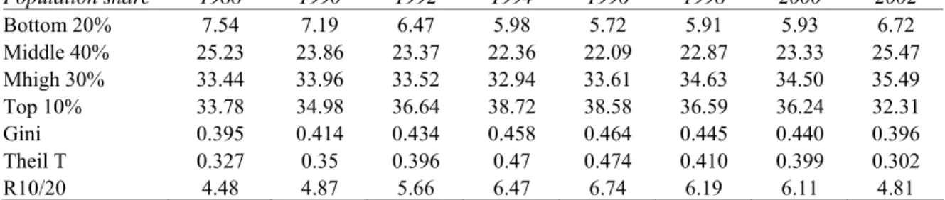
increased from 4.48 to 4.81 over the period 1988-2002, reaching a maximum of 6.74 in 1996. The Theil T index exhibited a slight decline from 0.327 in 1988 to 0.302 in 2002 (after peaking at 0.474 in 1996), but this may be due to the nature of this measurement, which is more sensitive to changes in the income distribution and tends toward greater variability than the Gini or other techniques.

Table 2.1 Inequality Indexes for the Distribution of Earnings, 1988–02

Population share 1988 1990 1992 1994 1996 1998 2000 2002 Bottom 20% 7.54 7.19 6.47 5.98 5.72 5.91 5.93 6.72 Middle 40% 25.23 23.86 23.37 22.36 22.09 22.87 23.33 25.47 Mhigh 30% 33.44 33.96 33.52 32.94 33.61 34.63 34.50 35.49 Top 10% 33.78 34.98 36.64 38.72 38.58 36.59 36.24 32.31 Gini 0.395 0.414 0.434 0.458 0.464 0.445 0.440 0.396 Theil T 0.327 0.35 0.396 0.47 0.474 0.410 0.399 0.302 R10/20 4.48 4.87 5.66 6.47 6.74 6.19 6.11 4.81

2.1 Earnings Inequality. Three broad hypotheses frequently are advanced to explain the

earnings inequality experienced in Mexico and other countries.1 These link earnings inequality to (a) increased openness of the economy, (b) institutional changes in the labor market, and (c) skill-biased technological change.

The first of these hypotheses argues that as trade barriers are reduced, an economy is placed under heightened competitive pressure to specialize along its lines of comparative advantage. A developed country with a relatively abundant supply of high-skilled workers, like the United States, will be induced to specialize in activities that require a high level of skill or education as its low-skilled industries come under increased competitive pressure from countries with an abundant supply of low-skilled, low-wage workers.

Hanson and Harrison (1995) examine the impact of Mexican trade reform on the structure of wages using information at the firm level. They test whether trade reform shifted employment toward industries that are relatively intensive in the use of skilled labor (the Stolper–Samuelson-Type [SST] effect, which is examined under NAFTA in Burfisher (1993) and others). They conclude that the wage gap was associated with changes within industries and firms, which cannot be explained by the SST effect. Thus the increase in wage inequality was due to other factors. Hanson (1997) examines a trade theory based on increasing returns, which has important implications for regional economies, and concludes that employment and wage patterns are consistent with the idea that access to markets is important for the location of industry.

1993, and to almost 78 percent in 1996. Since Mexico has an abundant supply of low-skilled labor compared with its northern neighbors, the liberalization of trade could be expected to induce a pattern of specialization that would raise the relative demand (and hence wages) of the lesser-educated members of the labor force. This did not happen. Instead, the increase in earnings inequality observed in Mexico followed the same pattern as that observed in the United States: less-educated workers experienced real wage declines, while highly educated workers experienced real wage improvements. The trade-based explanation may still be relevant, however, to the extent that greater openness facilitates the transfer of ideas and technology. This is a more persuasive explanation of the increase in earnings inequality. A variant of the globalization-technology nexus advanced by Feenstra and Hanson (1996) involves outsourcing in which multinational enterprises in the developed country relocate their less skill-intensive activities to the less skill-abundant developed countries. However, what is referred to as a low-skill activity in the United States may be a high-skill activity in Mexico, which could explain the similarity in the evolution of earnings inequality in both countries (de Ferranti et al., 2003).

The second explanation revolves around institutional changes such as reductions in the minimum wage, the weakening of trade unions, and the decline of state-owned enterprises. The existence of a binding minimum wage, for example, truncates the lower end of the wage distribution. As the minimum wage is allowed to erode—say, through inflation—it becomes less binding by moving farther down the low end of the wage distribution, with the result that, ceteris paribus, a higher share of wages will lie below the previous minimum-wage level. This translates into an increased dispersion in wages and earnings. Institutional developments have not exerted a significant influence on the earnings distribution since the early 1980s (see Hernández, Garro, and Llamas, 1997). The distribution of real wages, for example, does not reveal any significant distortions

account. This also renders any erosion of union power irrelevant for the distribution of earnings. In conclusion, although the influence of institutional factors cannot be rejected entirely, it does not appear to be the principal cause of the increase in earnings inequality.

A persuasive explanation, both for the United States and for Mexico, seems to be one that links earnings inequality to skill-biased technological changes that raise the relative demand for higher-skilled labor. Cragg and Epelbaum (1996) examine the shift in demand in Mexico. They point out that the major source of rising inequality is a biased shift in demand rather than a uniform growth in demand when there are different labor supply elasticities. Meza (1999) also investigates shifts in demand and offers the hypothesis that the shift in demand toward a more educated labor force “within” an economic sector explains the increase in their premium when compared with the shift in demand for less-educated workers “between” economic sectors. Tan and Batra (2000) study the skill-biased technical change hypothesis as a plausible explanation of wage inequality using data at the firm level for Colombia, Mexico, and Taiwan (China). They obtain the following results: (a) a firm’s investments in technology have the largest impact on the distribution of wages for skilled workers, (b) they have the smallest impact on wages paid to unskilled workers, and (c) wage premiums paid to skilled workers are led primarily by the firm’s investments in research and development (R&D) and training. Such conclusions seem to support the skill-biased technological change hypothesis, although these results should be considered carefully, since the analysis is based on data at the firm level and only for the manufacturing industry. According to the typology used by Johnson (1997), the type of technological change that drives wages up for the more highly skilled workers and drives wages down for the less-skilled workers (as occurred in both the United States and Mexico) is extensive skill-biased technological change. Under

explanations deals explicitly with changes in the distribution of education or with the

interaction between the educational policies that induced them and the workings of the labor market, which is the focus of this document.

2.2 Evolution of Educational Attainment. Levels of educational attainment have increased

rapidly in most developing countries since the 1950s (Schultz, 1988). Although Mexico also benefited from that development, there was a significant lag in its educational indicators. Londoño (1996), for example, points to an “education deficit,” according to which Latin American countries in general, and Mexico in particular, have approximately two years less education than would be expected for their level of development. Elías (1992) finds that education was the most important source of improvement in the quality of labor in Latin America between 1950 and 1970, although such improvements did not take place to the same extent in Mexico as in other countries in the region. This changed dramatically in the 1980s. Figure 2.1 shows that, although Mexico’s educational attainment increased steadily after the 1970s, it remained below the international trend line. In the 1980s, however, the growth of educational attainment in Mexico accelerated, permitting it to catch up with international standards by 1990, where its placement in Figure 2.1 is slightly above the trend line.

Figure 2.1 Cross-Country Relation between Educational Attainment and GDP, 1960–90 0 2 4 6 8 10 12 5 .0 0 6 .0 0 7 .0 0 8 .0 0 9 .0 0 1 0 .0 0 L n (G D P p er cap ita) A verage year s of school in g M ex ico 1 9 6 0 M ex ico 1 9 7 0 M ex ico 1 9 8 0 M ex ico 1 9 9 0

Note: The scatter diagram is based on 317 observations from five years. The trend line represents the least squares regression line given by S = -13.17 + 2.28 Ln(GDPcap) Adjusted R2 = 0.68.

(-18.7) (26.0) t-values in parentheses

The application of Ramsey’s RESET test to this regression equation failed to detect a specification error; unlike with the alternative specification of the following type: S = a + bX + cX2.

The closure of Mexico’s education gap vis-à-vis the rest of the world was hastened in part by the country’s economic stagnation. Mexico’s real GDP per capita in the mid-1990s was roughly the same as it had been in the first half of the 1980s. Nevertheless, this should not detract from the remarkable increase in schooling that occurred during the 1980s. While the level of average schooling in Mexico increased by roughly a year per decade during 1960–80 (from 2.76 to 4.77 years), it increased by two years in the decade of the 1980s. This acceleration in schooling was the product of concerted efforts to increase the coverage of basic education, combined with advances made in the reduction of primary school repetition and dropout rates. The observations pertaining to Mexico, ordered by date, are shown below in Table 2.2.

Table 2.2 Years of Schooling and Gross Domestic Product per Capita in Mexico, 1960–90 Year Average schooling (years) Ln (GDP per capita in 1980 U.S. dollars) 1960 2.76 7.95 1970 3.68 8.29 1980 4.77 8.71 1985 5.20 8.63 1990 6.72 8.67

Source: Calculations based on Barro and Lee data set. The World Bank.

With respect to changes in the distribution of schooling by socioeconomic groups, there are several aspects to be considered. In particular, three are examined here: the changes in this distribution that are related to gender, economic sector, and age.

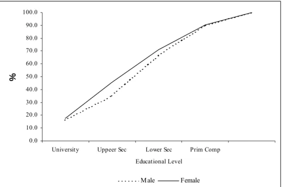
Table 2.3 shows the distribution of schooling by gender from 1988 to 2002. Even though there were clear improvements for both males and females, which signify an upgrade of educational attainment, women achieved a better performance during that period, especially at the top of the distribution. Improvements for males, in contrast, were spread more evenly over the entire distribution. Nevertheless, in 2002 women were undoubtedly more educated than men, as their cumulative distribution dominated that of men (see Figure 2.2).

Table 2.3 Educational Distribution by Gender, 1988, 1997 and 2004 (percentage) Educational Group Primary incomplete Primary complete Lower secondary complete Upper secondary complete University complete 1988 Male 19.0 30.1 24.5 14.6 11.8 Female 17.3 22.2 23.2 29.1 8.2 Total 18.5 27.7 24.1 18.9 10.7 1996 Male 13.3 26.2 27.6 17.8 15.1 Female 12.3 20.9 21.8 29.2 15.8 Total 12.9 24.4 25.7 21.6 15.4 2002 Male 10.1 23.3 31.5 18.8 16.2 Female 9.7 19.2 25.4 28.1 17.6 Total 10.0 21.9 29.5 21.9 16.7

Source: Calculations based on the ENEU survey (third quarter).

Figure 2.2 Cumulative Educational Distribution by Gender, 1997

0.0 10.0 20.0 30.0 40.0 50.0 60.0 70.0 80.0 90.0 100.0

University Uppeer Sec Lower Sec Prim Comp Educational Level

%

M ale Female Source: Calculations based on ENEU data.

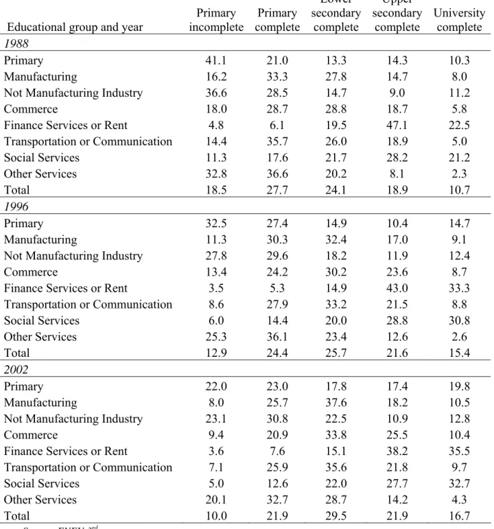
With respect to the distribution of schooling by economic sector, Table 2.4 shows large heterogeneity in the distribution of schooling across sectors from 1988 to 2002. The results suggest that within this heterogeneity, the financial sector uses a more highly skilled labor force. It seems that the primary sector, together with “Other services” sector, employ a more low-skilled labor force. Third, commerce is very heterogeneous in its labor force composition.

Table 2.4 Educational Distribution by Economic Sector, 1988, 1996, 2002

Educational group and year

Primary incomplete Primary complete Lower secondary complete Upper secondary complete University complete 1988 Primary 41.1 21.0 13.3 14.3 10.3 Manufacturing 16.2 33.3 27.8 14.7 8.0

Not Manufacturing Industry 36.6 28.5 14.7 9.0 11.2

Commerce 18.0 28.7 28.8 18.7 5.8

Finance Services or Rent 4.8 6.1 19.5 47.1 22.5

Transportation or Communication 14.4 35.7 26.0 18.9 5.0 Social Services 11.3 17.6 21.7 28.2 21.2 Other Services 32.8 36.6 20.2 8.1 2.3 Total 18.5 27.7 24.1 18.9 10.7 1996 Primary 32.5 27.4 14.9 10.4 14.7 Manufacturing 11.3 30.3 32.4 17.0 9.1

Not Manufacturing Industry 27.8 29.6 18.2 11.9 12.4

Commerce 13.4 24.2 30.2 23.6 8.7

Finance Services or Rent 3.5 5.3 14.9 43.0 33.3

Transportation or Communication 8.6 27.9 33.2 21.5 8.8 Social Services 6.0 14.4 20.0 28.8 30.8 Other Services 25.3 36.1 23.4 12.6 2.6 Total 12.9 24.4 25.7 21.6 15.4 2002 Primary 22.0 23.0 17.8 17.4 19.8 Manufacturing 8.0 25.7 37.6 18.2 10.5

Not Manufacturing Industry 23.1 30.8 22.5 10.9 12.8

Commerce 9.4 20.9 33.8 25.5 10.4

Finance Services or Rent 3.6 7.6 15.1 38.2 35.5

Transportation or Communication 7.1 25.9 35.6 21.8 9.7

Social Services 5.0 12.6 22.0 27.7 32.7

Other Services 20.1 32.7 28.7 14.2 4.3

Total 10.0 21.9 29.5 21.9 16.7

contrast the cohort and time effects, the latter referring to the comparison of the same age group at two different points of time.

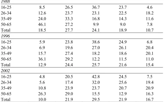
In order to do this, one can look at the first age groups, 16–25 and 26–34, like synthetic cohorts. Namely, the 26–34 age group in 1996, 2002 can be compared directly to the 16– 25 age group in 1988, and, to a lesser extent, the 35–49 age group in 1996, 2002 can be compared to the 26–34 age group in 1988. From 1988 to 1996 and to 2002, the percentage of persons in the category of incomplete primary schooling decreased, and this decline was higher than that experienced by the 16–25 age group (who were in the 26–34 age group in 1996). The opposite took place for the highest level of instruction. In other words, improvements throughout the educational process in Mexico were significant, both for those entering the system (higher coverage) and for those already in it (higher efficiency).

Table 2.5 Educational Distribution by Age Group, 1988, 1997 and 2002

Age group Primary incomplete Primary complete Lower secondary complete Uppeer secondary complete University complete 1988 16-25 8.5 26.5 36.7 23.7 4.6 26-34 12.6 23.7 23.1 22.5 18.2 35-49 24.0 33.3 16.8 14.3 11.6 50-65 46.1 27.2 9.9 9.0 7.8 Total 18.5 27.7 24.1 18.9 10.7 1996 16-25 5.9 23.8 38.6 24.9 6.8 26-34 6.9 19.6 27.0 26.1 20.4 35-49 15.7 27.4 18.2 18.6 20.1 50-65 36.1 29.2 12.2 11.5 11.0 Total 12.9 24.4 25.7 21.6 15.4 2002 16-25 4.8 20.5 42.8 24.5 7.5 26-34 5.6 17.4 32.0 25.6 19.4

between different age groups to that of inequality within synthetic cohorts and in relation to education. The results indicate that differences in both educational attainment and distribution among cohorts have become pronounced in recent times, leading to a higher (negative) correlation between education and age.

In 2000 adults in households in the top quintile had almost eight years more education than those in the bottom quintile (de Ferrati el al, 2004). This was the largest difference of the set of countries with comparable data in Latin America, and had actually risen by half a year since 1992. At the bottom of the distribution one dimension of this is the level of illiteracy. Whereas self-reported illiteracy rates are less than five per cent in the top two quintiles, they were 30 percent in the bottom quintile in 2000, down from 34 percent in 1992 (for the second quintile illiteracy declined from 17 per cent in 1992 to 13 percent in 2000). The evidence on educational dynamics is mixed. On one hand there was a modest reduction in the educational gap between the top and bottom quintiles of people in their fifties and thirties. There was also a small decline in the differences in enrollment from 13-17 year-olds between poor and rich households in the years spanning from 1992 to 2000. But there was a rise in differences in enrollments for 18-23 year-olds. Since the major divide in Mexico in terms of returns to education is now between those with and without tertiary education, rising inequalities at this level across incomes groups could be a source of further un-equalizing pressures in the coming years.

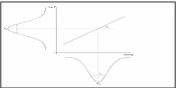
2.3 Evolution of Education and Earnings Inequality. In order to address the relationship

between education (the result of the interaction between supply and demand) and earnings inequality, it is necessary to explain how the labor market determines the earnings differentials among workers with different educational attributes. This relationship can be viewed as determined by two elements: (a) the distribution of education itself and (b) the way the labor market rewards educational attainment. The

Figure 2.3 shows the distribution of education in the horizontal axis (mt is an indicator of the average schooling of the labor force, and it represents its dispersion), while the vertical axis presents the distribution of earnings. The first quadrant depicts the interaction between the preexisting conditions (the distribution of education) and the workings of the labor market, through the steepness st of the income profile related to education. Therefore, at a point in time, (a) the higher mt is, the larger are the average earnings; (b) the lower it is, the smaller is the earnings inequality; and (c) the higher st is, the higher is the growth of preexisting disparities, and, accordingly, the higher is the earnings inequality. As these indicators change over time, they will induce changes in the income distribution: changes in it, assuming st constant, will change earnings inequality due to changes in the composition of the labor force (the so-called allocation-population effect), whereas changes in st will alter the earnings differentials (the income effect).

became much steeper. This means that there was a shift in demand toward highly skilled labor that was not met by an increase in supply. This probably occurred as a result of the accelerated pace of skill-biased technological change facilitated by the increased openness of the Mexican economy. The same pattern observed for the overall sample holds for the 16–25 age group: the mt rose from 0.476 in 1988 to 0.522 in 2002; the it increased from 0.066 to 0.077, whereas the st increased from 0.066 to 0.080.

Table 2.6 Synthetic Indicators of Schooling Distribution and Income Profile, 1988, 1997–02 Year 1988 1992 1996 2000 2002 mt 0.476 0.491 0.511 0.519 0.522

it 0.066 0.069 0.076 0.077 0.077

st 0.066 0.102 0.122 0.097 0.080

Source: Calculations based on the ENEU survey (third quarter).

3. METHODOLOGY

The dynamic decomposition analysis is a suitable tool for translating this stylized view into quantitative results, giving one a better understanding of the socioeconomic transformations responsible for changes in the earnings distribution. Besides permitting identification of the relevant individual variables, it also helps in understanding the nature of the contribution of each variable to the evolution of earnings inequality over time.

Ramos (1990), following Shorrocks (1980), shows that it is possible to break down the change in inequality between two points in time. This is done according to whether the change can be attributed to changes in the socioeconomic groups relative to incomes, to group sizes, or to internal inequalities, through use of the Theil T index. In generic terms, as shown before in a slightly different way, for a given partition of the population, the inequality indexes of this class can be written as:

I = I(αg, βg, Ig) (1)

among the groups (changes in the βs), with no direct changes in the group’s relative incomes (αs). The difference between this and what Knight and Sabot (1983) call the “compression” effect is that the present exercise includes the indirect change induced in I

through variation in the weighting of the Igs. Of course, the individual’s αs change as the

βs change, since the overall average income is altered. This indirect impact is also computed in the composition effect. The income effect corresponds to the changes in I

induced by changes in group incomes (αs), without changing the groups’ shares of the population (βs), and the internal effect is the change in the inequality caused only by modifications in dispersions at the group level (the Igs).2 The expressions corresponding to the Theil T index are derived in Annex 2.

4. FINDINGS

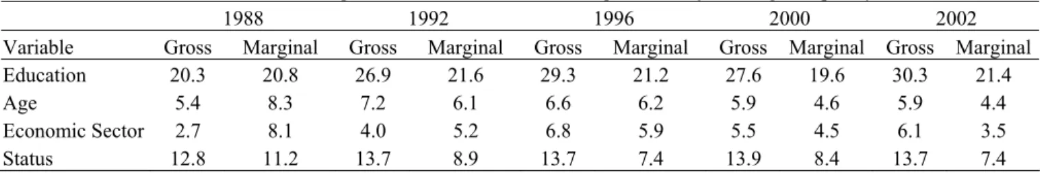
Education (the result of the interaction between demand and supply) is the variable that accounts for by far the largest share of earnings inequality in Mexico, in terms of both gross and marginal contributions. The gross contribution – that is, the

variable’s explanatory power when it is considered alone – amounted to one-fifth of total inequality in 1988 and one-third in 2002 (table 4.1). (In most earnings equations for any country, the set of all measurable observable variables explains at most 60 percent of the total variance. In the United States, education accounts for 10 percent of the total variance.) The marginal contribution – that is, the increase in the explanatory power when the variable is added to a model that already has the other variables – was remarkably stable and meaningful, remaining around 25 percent throughout the period. The difference between the two contributions has been growing over time, however, indicating that the degree of correlation with other variables has been increasing. This means that the “indirect” effects are becoming more important.

Table 4.1 Static Decomposition: Contribution to the Explanation of Earnings Inequality (%)

1988 1992 1996 2000 2002

Variable Gross Marginal Gross Marginal Gross Marginal Gross Marginal Gross Marginal Education 20.3 20.8 26.9 21.6 29.3 21.2 27.6 19.6 30.3 21.4 Age 5.4 8.3 7.2 6.1 6.6 6.2 5.9 4.6 5.9 4.4 Economic Sector 2.7 8.1 4.0 5.2 6.8 5.9 5.5 4.5 6.1 3.5 Status 12.8 11.2 13.7 8.9 13.7 7.4 13.9 8.4 13.7 7.4

The other variables considered seem to be much less important. All three of them, but particularly economic sector and status in the labor market, display an upward trend in their gross contribution and a declining trend in their marginal contribution. This can be interpreted as evidence that the interaction between these variables and education has become more intense. That is, the workers’ skills are becoming increasingly more relevant to the determination of their type of participation in the labor market as well as to their position across different economic segments of the economy. The same pattern holds when number of hours worked instead of sector is considered.

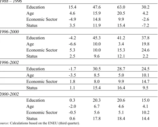
The results of the decomposition of the variations in the Theil T index for different intervals of time are shown in Table 4.2. First, when the variables are considered alone, education made the highest gross contribution to the changes in earnings distribution. Second, both the allocation and the income effect were positive in all periods. This means that changes in the distribution of education and in the relative earnings among educational groups were always in phase with alterations in the earnings distribution. Namely, when the income profile related to education became steeper and the inequality of education grew, the earnings distribution worsened as in all periods below.

Table 4.2 Results of the Dynamic Decomposition, 1988, 1996-02

Variable Allocation Income Gross Marginal

1988 – 1996 Education 15.4 47.6 63.0 30.2 Age 4.6 15.9 20.5 4.2 Economic Sector -4.9 14.8 9.9 -2.6 Status 3.5 11.9 15.4 -7.2 1996-2000 Education -4.2 45.3 41.2 37.8 Age -6.6 10.0 3.4 19.8 Economic Sector 5.3 10.0 15.3 24.6 Status 2.5 9.6 12.1 2.2 1996-2002 Education -1.7 30.5 28.7 24.5 Age -3.5 8.5 5.0 10.1 Economic Sector 1.8 8.0 9.9 14.7 Status 1.1 15.4 16.4 9.5 2000-2002 Education 0.3 20.3 20.6 15.0 Age -2.0 6.7 4.6 4.1 Economic Sector -0.5 5.6 5.1 10.2 Status 0.6 17.8 18.4 14.4

Source: Calculations based on the ENEU (third quarter).

Third, the income effect is always prevalent. If one considers, for instance, the 1988–96 period, changes in the relative earnings among educational groups alone would have generated a larger deterioration in the earnings distribution than the one observed. The same holds true for the other periods. Even the decrease in inequality observed in recent periods is explained by the changes in relative earnings (the income profile related to education became less steep as shown in Table 2.1). Therefore, it seems reasonable to conclude that the income effect is the leading force behind the increase in inequality, and this, in turn, suggests that the workings of the labor market and its interaction with educational policies should be thoroughly examined.

the influence of education is taken into account. In comparison, Székely (1995) finds that education and economic sector were significant factors in explaining inequality in the 1984–89 period, while education and job status were significant in the 1984–92 period. Bouillon, Legovini, and Lustig (1998) find that household characteristics explained 49 per cent of the increase in the Gini between 1984 and 1994, education being the most important characteristic.

The last period, from 1996 to 2002, deserves special comment. First, earnings inequality decreased. Second, once more, alterations were associated with education and such alterations appear to be the main factor responsible for the reduction in earnings inequality. As can be seen from the synthetic indicators, there were a small improvement in the distribution of schooling during the period and a sizable decrease in the steepness of the income profile related to education. All other variables, as observed for other periods, also contributed to an improvement in earnings inequality.

Table 4.3 shows the results of the same kind of decomposition for Brazil, Argentina, and Peru. The significance of education as an explanation of changes in inequality seems to be a common pattern in Latin American countries. Moreover, the relevance of the income effect over the allocation (population) effect is also shared by all countries where a similar analysis was carried out. In the Mexican case, however, the figures are higher than those for other countries (and in a shorter period of time). This means that changes in the structure of supply and demand for labor, which are greatly affected by the educational and macroeconomic policies followed by the country or by their interaction with the workings of the labor market, were particularly relevant for the earnings distribution.

Table 4.3 Education and Inequality Variation in Brazil, Argentina, and Peru

Country Study Time period

Explanatory power (per cent)a

Income effect (per cent)

Brazil Ramos and Trindade (1991) 1977–89 6–20 10–17 Argentina Fiszbein (1991) 1974–88 54–56 38–46 Peru Rodríguez (1991) 1970–84 32–47 34–43 a _{The income effect plus the allocation-population effect.}

4.1 Rates of Returns to Education. The earnings inequality evolution is not the result of

changes in the distribution of education, whereas the income profile, which is related to the returns to schooling, is the leading force in the explanation of inequality in Mexico. In light of this evidence, this section analyzes the structure and evolution of the rates of returns to education. Returns for upper secondary rose sharply in the late 1980s and early 1990s and then fell after 1993. Returns to tertiary education continued to rise until 1996, before falling to levels that remained much higher than in the early 1990s (Figure 4.1). These results took into account the change in the ENEU 94 questionnaire and are consistent with rate of return patterns found by de Ferranti et al. (2003) and World Bank (2000a), as well as with estimates using the National Survey of Household Incomes and Expenditures, or ENIGH. 

Figure 4.1 Yearly Rates of Return to Education Level, Mexico Urban Areas, 1988-2002

0 % 2 % 4 % 6 % 8 % 1 0 % 1 2 % 1 9 8 8 1 9 8 9 1 9 9 0 1 9 9 1 1 9 9 2 1 9 9 3 1 9 9 4 1 9 9 5 1 9 9 6 1 9 9 7 1 9 9 8 1 9 9 9 2 0 0 0 2 0 0 1 2 0 0 2 Year ly Rates of Retur n P r i m a r y C o m p l e t e L o w e r S e c o n d a r y C o m p l e t e U p p e r S e c o n d a r y C o m p l e t e T e r t i a r y C o m p l e t e  

Note: The yearly rate of return represents the additional contribution to wages from an additional year of a certain level of education. All the coefficients are statistically significant at the 5 per cent level and conditioned on age, squared age, gender, region (North, Center, South, and Mexico City).

Source: Calculations using third quarter of the National Urban Employment Survey (ENEU) from 1988 to 2001 and third quarter and urban section of ENET 2002.

A more complex pattern of changes in rewards to education is illustrated by an analysis that looks at different parts of the distribution (using quantile regression techniques — see Table 4.4). Returns are “convex” and become more so throughout the distribution until 1997 —that is they increased at a rising rate for higher levels of education. In 1988, when estimated at the median of the conditional earnings distribution tertiary education was associated with on average 52 per cent more income compared to a person with upper secondary complete education. By 1997, the premium to tertiary education had risen to 95 per cent. However, when estimated at the top of the distribution the premium to tertiary education “only” rose from 34 to 67 per cent (implying higher relative and

absolute returns to upper secondary in the upper reaches of the income distribution.) Moreover, while the premium to tertiary fell somewhat between 1997 and 2002 throughout most of the earnings distribution, they continued to rise at the top.

To test the robustness of these trends, four models were estimated: the basic model included only age, squared age, and gender; the second model was the basic model plus region; the third model added labor market status to the second; and the last model included all these variables plus sector of activity. 

Table 4.4 Marginal value of education by level along the conditional earnings distribution, Mexico 1988-2002

1988 1992

Quantile 0.1 0.25 0.5 0.75 0.9 0.1 0.25 0.5 0.75 0.9

Primary Complete 1.11 1.09 1.06 0.95 0.85 1.02 1.01 0.95 0.81 0.67

Lower Secondary Complete 1.21 1.18 1.19 1.24 1.27 1.15 1.18 1.21 1.25 1.3

Upper Secondary Complete 1.11 1.18 1.24 1.25 1.37 1.17 1.2 1.25 1.32 1.38

Tertiary 1.43 1.5 1.52 1.47 1.34 1.61 1.68 1.75 1.7 1.6

1997 2002

Quantile 0.1 0.25 0.5 0.75 0.9 0.1 0.25 0.5 0.75 0.9

Primary Complete 1.12 1.13 1.13 1.11 1.05 1.14 1.1 1.1 1.08 1.04

Lower Secondary Complete 1.19 1.21 1.26 1.32 1.39 1.15 1.15 1.16 1.21 1.25

Upper Secondary Complete 1.15 1.22 1.27 1.35 1.42 1.13 1.15 1.21 1.28 1.34

Tertiary 1.75 1.91 1.95 1.83 1.67 1.67 1.82 1.91 1.87 1.73

Note: The marginal value is with respect to the previous education level. The asymptotic covariance matrix of the estimated coefficient vector in quantile regression is computed using the bootstrap method. All the coefficients are statistically significant at 5 per cent level and conditioned to age, squared age, gender, region (North, Center, South, and Mexico City).

Source: WB Staff estimates using third quarter of ENEU 1997 to third quarter and urban section of ENET 2002. 

With respect to gender and geographic area the results show that rates of return to tertiary education are higher for both urban and rural men compared to women, particularly in the upper tail of the conditional earnings distribution.

In sum, the returns to education increased in Mexico from 1988 to 1997, especially for higher levels of education and in the upper tail of the conditional earnings distribution. However, there was a reversal to this trend after 1997, especially for higher levels of education and in the middle and lower tail of the conditional earnings distribution. This may reflect a structural development, if expanding relative supplies of school-leavers are offsetting the secular tendency for rising relative demand for skills — especially at the tertiary level (see de Ferranti et al., 2004). Alternatively, it may reflect a cyclical fall in education premia in times of recession, which has also been observed in the data for Latin America (ibid). But for the present, the labor force patterns by labor force status and education are fully consistent with the equalizing patterns of income growth.

5. CONCLUSION

Even though the levels of educational attainment expanded very rapidly, Mexico experienced a pronounced increase in the degree of inequality over the 1980s and mid-1990s. Most of the deterioration in the distribution of income happened in the middle to late 1980s (1984–89). The early 1990s displayed little change in total current income inequality except for a slight trend toward deterioration. The trends in the distribution of earnings differ from the trends in the distribution of current income in two ways. First, the gains are not limited to the richest 10 percent, as those in the seven-, eight-, and nine-tenths of the distribution improved their relative earnings over the period by almost 2

Education is a key variable for our understanding of income and earnings inequality in Mexico. Education is by far the variable that accounts for the largest share of earnings inequality in Mexico, in terms of both its gross and its marginal contribution. The marginal contribution of education to the explanation of inequality in Mexico is almost equal to the joint contribution of other relevant variables such as age, economic sector, labor market status and hours worked. It is worth pointing out that the difference between the gross and marginal contributions has been increasing over time, indicating that, as the economy progresses, education becomes even more important in determining the choices of sectors and occupations. That is, the workers’ skills are becoming increasingly relevant in determining their type of participation in the labor market as well as their position across different economic segments of the economy. The contribution of education to income inequality in Mexico is the second highest in Latin America, next only to Brazil. Moreover, what seems to be particularly interesting in the Mexican experience is that the significance of education has been increasing over time.

The contribution of relevant variables to changes in inequality for different intervals of time shows the following facts. First, education has the highest gross contribution in explaining changes in earnings distribution. Second, both changes in the distribution of education and in the relative earnings among educational groups have always been in phase with the alterations in the earnings distribution. Specifically, when the income profile effect related to education became steeper and the inequality of education increased, the earnings distribution worsened (as in the 1988-1996 period). Third, changes in the relative earnings among educational groups are always the leading force behind changes in inequality.

6. REFERENCES

Abadie, A. (1997). Changes in Spanish Labor Income Structure during the 1980’s: A Quantile Regression Approach. Investigaciones Económicas, 21(2), 253-72.

Altimir, O., and S. Piñera. (1982). Análisis de Descomposición de Las Desigualdades de Ingreso en la América Latina. Trimestre Económico, 49(196), 813–60.

Barros, R. and J. Almeida Reis. (1991). Wage Inequality and the Distribution of Education: A Study of the Evolution of Regional Differences in Inequality in Metropolitan Brazil.

Journal of Development Economics, 36, 117–43.

Bouillon, C., A. Legovini, and N. Lustig. (1998). “Rising Inequality in Mexico: Returns to Household Characteristics and the Chiapas Effect.” IADB.

---. (1999). “Can Education Explain Income Inequality Changes in Mexico?” IADB. Bourguignon, F. (1979). Decomposable Income Inequality Measures. Econometrica, 47(4),

901–20.

Bourguignon, F., M. Fournier, and M. Gurgand. (1998). “Labor Incomes and Labor Supply in the Course of Taiwan’s Development, 1979–1994.” The World Bank. Processed. Buchinsky, M. (1994). Changes in the U.S. Wage Structure 1963-1987: Application of

Quantile Regression. Econometrica, 62(2), 405-58.

---. (1995). Quantile Regression, Box-Cox transformation model and the U.S. wage structure, 1963-1987. Journal of Econometrics, 65, 109-54.

---. (1998). Recent Advances in Quantile Regression Models: A Practical Guideline for Empirical Research. Journal of Human Resources, 33(1), 88-126.

Burfisher, M. et al. (1993). Wage Changes in a U.S.-Mexico Free Trade Area: Migration Versus Stolper–Samuelson Effects. Working Paper 645. University of California, Berkeley, Department of Agricultural and Resources Economics. Processed.

Cowell, F. (1980). On the Structure of Additive Inequality Measures. Review of Economic Studies, 47, 521–31.

Cragg, M., and M. Epelbaum. (1996). Why Has the Wage Dispersion Grown in Mexico? Is It the Incidence of Reforms or the Growing Demand for Skills? Journal of Development Economics, 51(47), 99–116.

Elías, J. (1992). Sources of Growth: A Study of Seven Latin American Economies. International Center for Economic Growth. Processed.

Feenstra, R., and H. Hanson. (1996). Globalization, Outsourcing, and Wage Inequality.

AEA Papers and Proceedings, 86(2), 240–45.

Fields, G. (1996). Accounting for Income Inequality and Its Change. Cornell University. Paper prepared for presentation at the American Economic Association annual meetings, New Orleans, La. Processed.

Fiszbein, A. (1991). An Essay on Labor Markets and Income Inequality in Less Developed Countries. Ph.D. diss. University of California, Berkeley.

Hanson, H. (1997). Increasing Returns, Trade, and the Regional Structure of Wages.

Economic Journal, 107(440), 113–33.

Hanson, H., and A. Harrison. (1995). Trade, Technology, and Wage Inequality. Working Paper 5110. National Bureau of Economic Research. Cambridge, Mass. Processed. Hernández Laos E, N. Garro, and I. Llamas. (1997). Productividad y Mercado de Trabajo

en México. Processed.

Inter-American Development Bank. Informe (1998 – 1999). América Latina Frente a la Desigualdad: Progreso Económico y Social en América Latina.

Johnson, G. (1997). Changes in Earnings Inequality: The Role of Demand Shifts. Journal of Economic Perspectives, 11(2, spring), 41–54.

Juhn C., K. Murphy, and B. Pierce. (1993). Wage Inequality and the Rise in Returns to Skill. Journal of Political Economy, 3(3), 410–48.

Knight, J. T., and R. H. Sabot. (1983). Educational Expansion and the Kuznets Effect.

American Economic Review, 73, 1132–36.

Leibbrandt, M. V., Christopher D. Woolard, and Ingrid D. Woolard. (1996). The Contribution of Income Components to Income Inequality in South Africa. Living Standards Measurement Study. Working Paper 125. World Bank, Washington, D.C.

Processed.

Londoño, J. L. (1996). Poverty, Inequality, and Human Capital Development in Latin

America, 1950–2025. World Bank, Latin American and Caribbean Studies,

Washington, D.C. (June). Processed.

Lopez-Acevedo, G, and M. Walton. (2004). Mexico Poverty Assessment. Washington: The World Bank.

Lopez-Acevedo, Gladys. (1997). Learning Achievement and School Cost Effectiveness in Mexico: The Case of the Pare Program. Working Policy Research Paper, The

Lopez-Acevedo and Salinas. (2000b). Factors that Affect Learning Achievement in Mexico: The Case of Mexico D.F., Nuevo Leon and Tabasco. The World Bank, Mimeo.

Lustig, N., and M. Székely. (1996). Mexico: Evolución Económica, Pobreza y Desigualdad. Processed.

Meza, L. (1999). Cambios en la estructura salarial en Mexico en el periodo 1988-1993 y el aumento en el rendimiento de la educacion superior. Trimestre Económico, 49(196),

813–60.

Montenegro, Claudio E. (1999). The Structure of Wages in Chile 1960-1996: An Approach of Quantile Regressions. Economics Letters, 60(2), 229-35.

Moreno, A. (1989). La distribución del Ingreso Laboral Urbano en Colombia: 1976–1988.

Desarrollo y Sociedad (Bogotá) 24.

Muller, R. (1998). Public-Private Sector Wage Differentials in Canada: Evidence from Quantile Regressions. Economics Letters, 60(2), 229-235.

Pánuco-Laguette, H, and M. Székely. (1996). Income Distribution and Poverty in Mexico. In Victor Bulmer-Thomas (Ed.), The New Economic Model in Latin America and Its Impact on Income Distribution and Poverty (pp. 185-222). New York: St. Martin’s

Press.

Psacharopoulos, G. (1993). Returns to Investment in Education: A Global Update. Policy Research Paper 1067. World Bank, Policy Research Department, Washington, D.C. (January). Processed.

Psacharopoulos, George, S. Morley, Albert Fiszbein, H. Lee, and B. Wood. (1992). Poverty and Income Distribution in Latin America: The Story of the 1980s. World Bank, Washington, D.C. Processed.

Ramos, L. (1990). The Distribution of Earnings in Brazil: 1976–1985. Ph.D. diss.,

University of California, Berkeley.

Ramos, L, and C. Trindade. (1992). Educação e desigualdade de salários no Brasil: 1977/89. In Perspectivas da Economia Brasileira 1992. Rio de Janeiro: IPEA.

Reis, J. and R. Paes de Barros. (1989). “Um estudo da evolução das diferenças regionais da desigualdade no Brasil.” Rio de Janeiro: IPEA. Processed.

Reyes, A. (1988). Evolución de la distribución del ingreso en Colombia. Desarrollo y Sociedad, 21.

1369–84.

Shorrocks, A. F., and J. E. Foster. (1985). Transfer Sensitive Inequality Measures. Review of Economic Studies, 5, 105–38.

Shorrocks, A. F., and D. Mookherjee. (1982). A Decomposition Analysis of the Trend in U.K. Income Inequality. Economic Journal, 92, 886–902.

Shultz P. and E. Mwabu. (1996). Symposium Issue on How International Exchange, Technology, and Institutions Affect Workers. The World Bank Economic Review, 11, 1

January.

Symposium on Wage Inequality. (1997). Journal of Economic Perspectives, 11(2), spring.

Székely, M. (1995). Aspectos de la desigualdad en México. Trimestre Económico LXII,

246, 201–43.

Tan, H, and Geeta Batra. (2000). Technology and Firm Size-Wage Differentials in Colombia, Mexico, and Taiwan (China). The World Bank Economic Review, 11(1), 59–

83.

Vieira, M. L. P. (1998). A relação entre educação e desigualdade no Brasil. Master’s diss. EPGE, Rio de Janeiro.

World Bank. (1996). World Development Report 1996. Washington, D.C.: Oxford

University Press.

World Bank. (2004). Mexico: Public Expenditure Review. Washington, D.C..

World Bank. (2004). Mexico: Income Generation and Social Protection for the Poor. Washington, D.C..

World Bank. (2006). Virtuous Circles of Poverty Reduction and Growth 2006.

ANNEX 1 ENEU

This paper uses information from the National Urban Employment Survey (ENEU), which is also a micro-level data set collected by (National Institute of Statistics and Geography of Mexico) INEGI and contains quarterly wage and employment data over 1987-2002. According to INEGI’s methodology document on the ENEU, the data are representative of the 41 largest urban areas in Mexico, covering 61 percent of the population in urban areas with at least 2,500 inhabitants and 92 percent of the population living in metropolitan areas with 100,000 or more inhabitants. In 1985 the ENEU included 16 urban areas: Mexico City, Guadalajara, Monterrey, Puebla, León, San Luis Potosí, Tampico, Torreón, Chihuahua, Orizaba, Veracruz, Mérida, Ciudad Juárez, Tijuana, Nuevo Laredo, and Matamoros, covering 60 percent of the urban population for that year. In 1992, 18 more urban areas were included in the survey: Aguascalientes, Acapulco, Campeche, Coatzacoalcos, Cuernavaca, Culiacán, Durango, Hermosillo, Morelia, Oaxaca, Saltillo, Tepic, Toluca, Tuxtla Gutiérrez, Villahermosa, Zacatecas, Colima, and Manzanillo. In 1993 and 1994 Monclova, Querétaro, Celaya, Irapuato, and Tlaxcala entered the ENEU. Finally, Cancún and La Paz joined the survey in 1996. According to INEGI, the ENEU always has covered about 60 percent of the national urban population.

The data are from household surveys, which fully describe family composition, human capital acquisition, and experience in the labor market (the variables contain information about social household characteristics, activity condition, position in occupation, unemployment, main occupation, hours worked, earnings, benefits, secondary occupation, and search for another job). As with the National Household and Income Survey (ENIGH), the sampling design was stratified in several stages (where the

Category Selection

The individuals in the sample were classified according to their educational level, age, sector of activity, position in occupation, hours worked, and geographic region in the following categories:

Educational level

a) Primary incomplete: no education and primary incomplete (one to five years of primary)

b) Primary complete: primary complete and secondary incomplete (one or two years) c) Secondary complete: secondary complete and preparatory incomplete (one or two years)

d) Preparatory complete: preparatory complete and university incomplete

e) University complete: university complete (with degree) and postgraduate studies

Age a) 12 to 25 years old b) 26 to 34 years old c) 35 to 49 years old d) 50 to 65 years old Sector of activity

a) Primary sector (includes agriculture, forestry, fishing, and mining). b) Manufacturing industry

c) Nonmanufacturing industry (includes construction and utilities) d) Commerce

e) Finance services and rent

Labor market status a) Employer b) Self-employed

c) Informal salaried: people who work in an enterprise with 15 or fewer workers and do not receive social security (IMSS, ISSTE, private, and so forth)

d) Formal salaried: people who work in an enterprise with 16 or more workers or receive social security (IMSS, ISSTE, private, and so forth)

e) Contract

Hours worked

a) 20 to 39 hours a week b) 40 to 48 hours a week c) At least 49 hours a week

Geographic regions

a) North: Baja California, Baja California Sur, Coahuila, Chihuahua, Durango, Nuevo León, Sinaloa, Sonora, Tamaulipas, and Zacatecas

b) Center: Aguascalientes, Colima, Guanajuato, Hidalgo, Jalisco, Mexico, Michoacán, Morelos, Nayarit, Puebla, Querétaro, San Luis Potosí, and Tlaxcala

c) South: Campeche, Chiapas, Guerrero, Oaxaca, Quintana Roo, Tabasco, Veracruz, and Yucatán

d) Distrito Federal.

e) Having positive earnings4

Annex 2. Methodological Note

Gini Index

The Gini index is defined by

) 1 ( )] ( , cov[ 2 μ Y F Y GI =

where Y is the distribution of per capita income Y = (y1, …, yn), where yi is the per capita income of individual i, I = 1, …, n;μ is the mean per capita income; F(Y) is the cumulative distribution of total per capita income in the sample (that is, F(Y)=[f(y1),…f(yn)], where f(yi) is equal to the rank of yi divided by the number of observations [n]).5

Equation 1 can be rewritten and expanded into an expression for the Gini coefficient that captures the “contribution to inequality” of each of the K components of income (see Leibbrandt and others 1996).

) 2 ( 1

∑

where Sk is the share of source k of income in total group income (that is, Sk = μk / μ), Gk is the Gini coefficient measuring the inequality in the distribution of income component k within the group, and Rk is the Gini coefficient of income from source k

The larger is the product of these three components, the greater is the contribution of income from source k to total inequality.

Theil T Index7

This index is calculated as follows:8

) 3 ( ln ⎟ ⎠ ⎞ ⎜ ⎝ ⎛ ⎟ ⎠ ⎞ ⎜ ⎝ ⎛ ⎟ ⎠ ⎞ ⎜ ⎝ ⎛

_∑

whereYi is the income of the ith individual, Y is average income, and n is

population size.

Static decomposition of the Theil index. If the population is divided into G groups with ng observations each, it is then possible to write equation 3 as:

) 4 ( ln 1 ⎟⎟ ⎠ ⎞ ⎜⎜ ⎝ ⎛ ⎟⎟ ⎠ ⎞ ⎜⎜ ⎝ ⎛ ⎟⎟ ⎠ ⎞ ⎜⎜ ⎝ ⎛

∑

∑

where Yig is the income of the ith individual of the gth population subgroup.

If we now define n n_g g = β and k Y Z g

g = where Yg is the average income of

the gth group and k is a reference income, it is possible to show, after some algebraic manipulation, that T can be expressed as:

where k = ΣβgZg and Tgis the Theil index for the gth group.

The first two terms on the right-hand side of equation 5 correspond to the between group inequality, and the third corresponds one to the within group inequality.

Choosing the mean income as the reference income—that is,

Y Y

Z g

g

g =α = —

expression 5 simplifies to:

) 6 ( ln _T

+

∑

∑

The first term in equation 6 is the between group inequality, and the second term is the within group inequality.

Dynamic decomposition analysis. By totally differentiating equation 6, we have:

) 7 ( T d T T + d T + d T = dT g g G 1 = g g g G 1 = g g g G 1 = g ∂ ∂ ∂ ∂ ∂ ∂

∑

∑

∑

The first term on the right-hand side is the population allocation effect (changes in T caused exclusively by population shifts). The second term is the income effect (changes in T induced exclusively by changes in standardized mean incomes), and the third one is the internal effect (changes in T caused by changes in internal dispersion).

) 10 ( β αg g g = T T ∂ ∂

Replacing equations 8, 9, and 10 into equation 7 and simplifying, we obtain

(

)

(

)

(

)

+

∑

∑

∑

The three terms on the right-hand side of equation 11 correspond to the allocation, income, and internal effects, respectively.

For estimation purposes, equation 11 must be approximated. The convention used in the empirical exercises is to evaluate the expression at the middle points.

Level, Inequality, and the Indicator of Steepness of the Income Profiles in Educational Level

Ramos (1990) uses three synthetic measures for the indicators m_t(average

schooling), it(schooling inequality), and st(income profile), based directly on the

definition of the Theil index.

The calculations of the principal parameters αg, βg, and Tg (5) could determine the changes in the distribution by level of education (g groups in this category). These parameters allow us to analyze the trend in educational income differentials, the distribution of the population in each educational level, and the inequality among them.

These measures can be calculated as follows:

∑

∑

∑

∑

∑

∑

∑

α is the standardized income of educational category g for the reference year, t

g

β is the fraction of the labor force in the gth educational category in year t, and *

g

β is the value βg in the reference year. s_tcan be understood as an indicator of the

relative steepness of the income profiles related to education. If one fixes the fraction of the labor force in each educational group, it follows that the steeper is the income profile, the larger is the between group inequality. it corresponds to the Theil T index that would

prevail in a population with no inequality within the educational groups and where the group incomes are proportional to the group average incomes in the base year.