An improved decision model for evaluating risks in construction projects
1Morteza Yazdani 1, M Reza Abdi 2 , Niraj Kumar 3* , Mehdi Keshavarz-Ghorabaee 4 and Felix T. S. 2
Chan5 3
4
1Universidad Loyola Andalucai, 41014, Seville, Spain. 5
email: [email protected] 6
2 Bradford School of Management, Emm Lane, Bradford, BD9 4JL, United Kingdom. 7
email: [email protected] 8
3 University of Liverpool Management School, Chatham Street, Liverpool L69 7ZH, United Kingdom 9
email: [email protected] 10
4Department of Industrial Management, Faculty of Management and Accounting, Allameh Tabataba’i 11
University, Tehran, Iran 12
email: [email protected] 13
5Department of Industrial and Systems Engineering, Hong Kong Polytechnic University, Hung Hom, 14 Hong Kong. 15 email: [email protected] 16 17 *Corresponding Author 18 19 20 21 22 23 24
25
Abstract 26
27
The paper develops an innovative risk evaluation methodology to address the challenges of multi-28
criteria decision-making problem of project evaluation and selection. The methodology considers 29
Fuzzy Analytic Network Process (FANP) to incorporate the inter-dependencies of different risk 30
factors, and Failure Mode and Effect Analysis to conduct the rating analysis of projects to develop the 31
decision matrix. Finally, evaluation based on the distance from average solution compares alternative 32
projects and reports the optimal solution. The proposed approach allows project managers to engage 33
in the evaluation process and to use fuzzy linguistic values in the assessment process. A case study 34
from the construction sector is selected to verify the efficacy of the proposed approach over other 35
popular approaches in literature. 36
Keywords: Multi-criteria decisions; Failure mode and effect analysis; Fuzzy analytical network 37
process; Risk assessment; Construction projects. 38
Introduction 40
41
In industrial projects, the risk assessment exercise has strategic importance, and can decide the success 42
or failure of the project. Risk assessment involves the analysis of the whole project in order to reduce 43
the impact of potential risk factors. It begins by identifying the potential risks that could influence the 44
project. During the project planning phase, the project manager usually forms a team of experts and 45
relevant stakeholders to assess the potential risk factors that could affect the successful completion of 46
the project. The team uses techniques like brainstorming, discussions and tools such as flowcharts, root 47
cause analysis, histogram and cause-effect analysis to release potential problems. Several tools are 48
utilized by different risk management teams to develop the risk-breakdown structure and risk-profile. 49
This paper is primarily focused on the risk evaluation and assessment of construction projects. 50
Scenario analysis is one of the most popularly used techniques for evaluating project risks. The project 51
team evaluates the impact of each risk factor in terms of the probability of its occurrence and the 52
influence on the project. A structured approach is needed to recognize potential / known failure modes 53
at different levels of the project and investigate the effect on the next sub-system level (Sharma et al. 54
2005). Failure Mode and Effect Analysis (FMEA) is considered as a fundamental tool and a part of the 55
risk assessment methodology in several studies, and is established as one of the most reliable 56
techniques (Dinmohammadi and Shafiee, 2013). This technique can help in understanding different 57
failure modes within a system, evaluating their impacts, and deciding for corrective actions 58
(Abdelgawad and Fayek, 2010). However, reported applications of this technique in the construction 59
industry are limited (Andery et al., 2000; Nielsen, 2002). Evaluating different risk factors in 60
construction projects is a complex task since the objective functions may change during the project life 61
cycle (Dikmen et al. 2008). Further, Tserng et al. (2009) discussed an ontology based risk management 62
framework for construction projects based on the project life cycle variance and covariance. However, 63
potential risks (Safari et al. 2016). In practice, it is necessary to address technical, external and internal 66
(organizational) issues through a risk breakdown structure. When developing this structure, it is 67
important to reduce the chance of a risk event being missed, and to develop a comprehensive view of 68 the project. 69 Research significance 70 71
Multi-criteria decision-making (MCDM) techniques are amongst the most efficient approaches to 72
evaluate risk factors and assist in real-life decision problems. In recent years, there is growing trend in 73
integrating different MCDM approaches to develop hybrid techniques with better performance to 74
address risk assessment problems in different projects (Chan and Kumar 2007; Chan et al. 2008; Chang 75
2013; Prakash and Barua, 2016). It enables experts to be flexible in choosing relevant methods and 76
creating integrated structures. Past literature (such as Gu and Zhu 2006; Tzeng et al. 2007; Yang and 77
Tzeng, 2011; Liu et al. 2012; Liu et al. 2013) have provided further evidence to support the novelty of 78
integrated and hybrid methods in order to take the advantage of two or more decision making 79
approaches. 80
Moreover, Franceschini and Galetto (2001) presented a multi-expert MCDM model to analyze the risk 81
preferences of failures in FMEA. In this model, risk factors were transformed as evaluation criteria, 82
while failure modes were considered as different alternatives to be decided. This method contemplated 83
each decision-making criterion as a fuzzy subset over the set of alternatives. Chin et al. (2009) 84
discussed a FMEA model using the group-based evidential reasoning (ER) approach to collate diverse 85
opinions and prioritize failure modes under uncertainties such as incomplete assessment, ignorance 86
and intervals. Hu et al. (2009) developed a green component risk priority number to analyze the risks 87
involved due to hazardous substances. In their study, Fuzzy analytic hierarchy process (FAHP) was 88
used to identify the relative weights of risk factors. Then the green component risk priority number 89
(RPN) was calculated for each component to assess the risks derived from them. In this study, the 90
application of fuzzy value FMEA in the context of risk evaluation is discussed, where FMEA forms 91
an initial decision matrix for evaluation process. 92
The novelty of the proposed approach lies in the way it analyzes the anatomy of a project framework. 93
One of the important activities in decision modelling is to find logical ways to weigh different decision 94
attributes. In past literature, mostly Analytic hierarchy process (AHP), Delphi and entropy based 95
approaches are used to determine the weights of different influencing factors. However, in many 96
decision problems, the decision criteria are strictly dependent on each other. Analytic network process 97
(ANP) is the method that undertakes the interrelationship of risk factors in a ratio scale and aids in 98
overcoming the drawbacks of the decision levels and clusters (Tavana et al. 2016). The advantages of 99
ANP can be summarized as follows (Ignatius et al. 2016) : 1) ANP converts qualitative values into 100
numerical values for relative analysis of preferences, 2) It has a simple and intuitive structure, and 3) 101
it allows the participation of stakeholders and experts in the decision process. 102
In addition, risk evaluation in real life problems usually confronts low levels of information and 103
certainty. In the literature, the fuzzy approach is recognized as an effective tool for tackling uncertainty 104
stemming from inaccurate information (Wang et al. 2009). In multi-criteria decision-making problems, 105
where some of the criteria cannot be quantitatively represented, the fuzzy set theory can be helpful to 106
enable project assessors to express their linguistic preferences, and to convert those preferences into 107
numerical values for comparative analysis (Ho et al. 2012). He et al. (2015) studied the complexity of 108
mega construction projects in China using Fuzzy ANP methodology and argued that the methodology 109
can help decision makers to develop effective strategy for the project execution. 110
In this paper, an integrated decision-making approach, combining ANP and FMEA in a fuzzy 111
environment is proposed for the risk evaluation process. Very limited studies are available in the 112
literature which attempt to integrate FMEA and ANP with fuzzy variables for risk assessment. 113
adopted to compare alternative projects and rank them based on risk priority. A case study is also 115
discussed to explain the implementation process of the proposed approach. 116
The rest of the paper is organized as follows: Next section discusses the proposed integrated approach 117
(combining fuzzy set theory, ANP and FMEA) for risk assessment. Further, the case study and risk 118
management methodology are presented, along with the analysis and findings. The managerial 119
implications of the proposed approach is also discussed. At the end, paper concludes with a discussion 120
on future research directions. 121
Research Background 122
This section discusses different methods for addressing multi-criteria decision-making problems. 123
Particular attention has been given to approaches that are closely related to the integrated approach for 124
risk evaluation proposed in this paper. 125
Fuzzy set theory 126
In real world decision problems, there are many instances where decision makers are faced with 127
multiple criteria when reaching to a decision. However, estimating the impact of these criteria on 128
potential decision outcomes is cumbersome, and this sometimes results in extremely pessimistic or 129
optimistic decisions being made. In every decision environment two types of systems can be proposed 130
based on the availability of information. In white systems, all internal information is completely 131
known, whereas in a black system, it is difficult to obtain any information and characteristics about the 132
system (Zavadskas et al. 2010). Saaty (1980) introduced the analytic hierarchy process (AHP) to 133
accurately represent the consensus of experts and is one of the most widely applied methods in practical 134
applications. In his study, the geometric mean is used as the reference for triangular fuzzy numbers. 135
Zadeh (1965) provided the fuzzy set theory for dealing with the uncertainty due to imprecise and vague 136
information. The theory also allows mathematical operations and programming to be applied in the 137
fuzzy domain. A fuzzy set is a class of objects with a continuum of grades of membership (degree of 138
compatibility) (Peng and Selvachandran 2017). Such a set is characterized by a membership function, 139
which reflects the degree of compatibility assigned to each object with the grade of membership 140
between 0 and 1. 141
A triangular fuzzy number (TFN) is defined simply as where parameters , and represent 142
the smallest possible value, the most promising value and the largest possible value that denotes a 143
fuzzy event. The triangular fuzzy numbers can be established as: 144
(1) 145
, (2) 146
To establish the fuzzy pair-wise comparison matrix, the following procedure must be followed: 147
Suppose denotes a triangular fuzzy number for depicting the relative importance of criteria 𝐶" 148
, 𝐶#,….𝐶$. In this way, represents a matrix constructed by triangular fuzzy numbers. 149
(3) 150
Defuzzification is a technique to convert the fuzzy number into crisp real numbers and the procedure 151
of defuzzification is to locate the Best Non-fuzzy Performance (BNP) value (Tsaur and Wang 2007). 152
Methods such as the Mean-of-Maximum, the Centre-of-Area, and the α-cut method are the most 153
common defuzzification approaches. In this research, fuzzy risk criteria are defuzzified with the help 154
of the Centre-of-Area method. This was chosen due to its simplicity and its less reliance on the personal 155
judgement of analysts. A defuzzified value of a TFN can be produced using the equation below: 156 BNP = (4) 157 158 Fuzzy ANP 159 ) , , (l mu l m, u ij a~ ) , , ( ~ ij u ij m ij l ij a = ij u ij m ij l £ £ lij,mij,uijÎ(0,1)
[ ]
aij A~= ~ ij a~[ ]
ú ú ú ú ú ú û ù ê ê ê ê ê ê ë é = = 1 2 ~1 1 ~1 2 ~ 1 12 ~1 1 ~ 12 ~ 1 ~ ~ 2 1 ! " " " " ! " n a n a n a a n a a C C C ij a A n ij L ij L ij M ij L ij U - )+( - )]/3+ [(their corresponding attributes (Saaty 1996). It helps in overcoming the drawbacks of AHP in 162
addressing interrelationships issues among different decision levels using a super-matrix which detects 163
the composite weights (Shyur, 2006; Kang et al. 2012). 164
By structuring the problem as an ANP model, the uncertain vague elements of matrix A used for pair-165
wise comparisons can be redefined by fuzzy membership functions reflecting the degree of 166
compatibility for both the quantitative and the qualitative criteria. By pair-wise comparisons using a 167
fuzzy membership function e.g. with triangular fuzzy numbers, the fuzzy pair-wise comparison matrix 168
𝐴& with elements 𝑎()*, is constructed where reflects the influence of element i over 169
element j that could be a criterion/alternative in the network with lower ( ), mean ( ) and higher 170
values respectively. The value could reflect the domain/degree of fuzziness. The greater 171
that is, the fuzzier the degree is. When , the judgment is a non-fuzzy number (crisp 172
value) with importance value. Contrarily, assuming that 𝐴& is a positive n × n reciprocal matrix, 173
that represents influence of element j over element i with lower , mean 174
, and higher values respectively. As a result, the fuzzification increases the complexity of the 175
computation for synthesis judgments based on the fuzzy elements .To be able to evaluate a fuzzy 176
ANP model through standard pair-wise comparisons, the fuzzy values are standardized into a single-177
pattern fuzzy set dealing with both linguistic and/or quantifiable criteria (Abdi, 2009). Accordingly, 178
the importance weights are defined with five triangular fuzzy sets: , , , , with their 179
corresponding lower, mean, and upper values defined in equation (5) and represented in Table 1 (Abdi 180 and Labib, 2004). 181 ) , , ( ~ ij u ij m ij l ij a = ij l mij ij u uij -lij ij l ij u - uij -lij =0 ij m ) 1 , 1 , 1 ( 1 ~ ~ ij l ij m ij u ij a ij a = - = ij u 1 ij m 1 ij l 1 s ij a ^ 1 3^ 5^ 7^ 9^
; Є (1, 1, 3) 182 ; Є (x-2, x, x+2) (5) 𝑎(*) = 183 ; Є (7, 9, 9) 184 185 186
<< Insert Table 1 about here >> 187
188
The fuzzy range of ( , , , , ) are used to express linguistic preferences for evaluation criteria in 189
terms of Equal (EQ), Low (L), Medium (M), High (H), and Very High (VH) as decision linguistic 190
variables (Table 1), respectively. EQ can also represent equal to very low importance. If criterion (ci) 191
is assigned one of the fuzzy numbers above when compared with criterion (cj), then cj has the reciprocal 192
value when compared with ci. To simplify the weighting process, the priority values are put in a 193
reciprocal comparison bar for each pair of attributes with respect to a criterion/alternative. For example, 194
if value 5 is assigned on the right-hand side criterion (cj), then criterion cj is more important than ci 195
with a moderate degree. Similarly, if value 5 is assigned on the left criterion (ci), then the criterion ci 196
is more important than cj with a moderate degree (Abdi and Labib, 2004). 197
The synthesized fuzzy degree of criterion i influenced by criterion j, where , each with a 198
triangular fuzzy number in an ANP structure, can be derived from formula (5). In the ANP with a 199
(n × n) super-matrix, in which any element can influence on another element based on the influence 200
flow from a component/cluster to another component/cluster, or from a component to itself (inner 201
dependency loop), the number of elements influencing on or being influenced by criterion i could be 202
up to n elements. In the fuzzy environment, the comparison ratios are represented by the 203
membership functions that indicate the degree of compatibility/possibility. 204 ^ 1 ^ x ^ 9 ^ 1 3^ 5^ 7^ 9^ n j i, =1,2,...., ij a~ ij a ~
Fuzzy FMEA 206
Failure mode and effects analysis (FMEA) is a risk measurement tool, which is used in various 207
engineering and management problems such as project risk management. Accordingly, a risk priority 208
number (RPN) is constructed for measuring key risk elements and prioritizes several risky 209
problems/projects, for which the largest RPN corresponds to the riskiest problem/project being 210
considered. The purpose of this section is to explain the logic and shortcomings of RPN values. 211
In the FMEA, risk value is evaluated by grading the data according to key risk elements: 1) severity of 212
effect (S), 2) frequency of occurrence (P), and 3) detectability (D). The multiplied sum of these figures 213
produces the risk priority number. Failure mode and effects analysis extends the risk priority matrix 214
that includes RPN for each project: 215
(6) 216
In typical RPN problems, a rating of 1 to 10 on each scale will be assigned to each risk element, with 217
10 being severe, very likely to occur, and impossible to detect. These ratings are then multiplied 218
together to obtain RPN values, which are used to assess the projects. The idea is that the problem with 219
the highest RPN value is the critical one (with a highest priority) that needs to be focused on. However, 220
there are two logical difficulties with calculating the RPN. As argued by Wheeler (2011), 221
multiplication of the RPN elements is nonsense; with having assigned a range of 1 to 10 to each 222
element, RPN varies from 1 to 1,000 with only 125 possible values, which are not uniformly distributed 223
between 1 and 1,000. In the typical RPN, the three elements are assumed to be of the same importance 224
while being given crisp values ranging from 1 to 10. RPN values gained from multiplication of the 225
three elements are not meaningful because each value is an interval scale and not a ratio scale as a 226
requirement for multiplication. However, in a ratio scale, the values can be ordered with consistently 227
identical distance between two values (the distance between 1 and 3 is the same of the distance between 228
5 and 7, and etc.), and with an absolute zero point (starting from zero rather than 1). 229 Detection × y Probabilit × Severity = RPN
To overcome the shortcomings of using certain value and illogical multiplication, the elements can be 230
considered as linguistic values ranging from Very Low (VL), Low (L), Medium (M), High (H), and 231
Very High (VH) respectively. By using RPN linguistic scores, 125 problem descriptions (53) can be 232
obtained; each with the 5 options above e.g. a risk score of HMH (High, Medium High) reflect values 233
of (Severity, Occurrence, Detectability) respectively. So far, all the values for RPN elements are 234
assumed to be crisp ranging in [1,5]. Conversely, the elements can be considered as criteria with fuzzy 235
number as described earlier. Therefore, the fuzzy range of ( , , , , ) can be used to express 236
linguistic priorities. Using fuzzy number ranging from , , , , to , each problem description can 237
be seen as a fuzzy linguistic value, and a ratio fuzzy scale can be achieved by a synthesized fuzzy 238
number. Adopting from the extent analysis (Chang, 1996), the synthesized result for criterion i will 239
remain fuzzy as shown in formula (7). 240
(7) 241
V (M ≥ L) = supreme x ≥ y [min µL (x), µ M (y)] (8) 242
Where V is the possibility of M ≥ L and a pair (x,y) exists, If x≥ y and µL (x) = µ M (y) =1, then V( M 243
≥ L ) =1 where V is the possibility distribution. Considering M and L are convex fuzzy numbers 244 (𝑙, 𝑚, 𝑢) and L= (1,3,5) and M= (3,5,7): 245 V( M ≥ L ) =1 as mM= 5 and ≥ mL= 3 (9) 246 V( L ≥ M ) = µL (d) =D = 0.5 (10) 247
D is equal to µ (d), and d is the intersection point of two sides of triangles of fuzzy number M and L. 248
we have: 249
Line 1: p1: (5,0), p2: ( 3,1) then (Y-0)/(1-0) = (X- 5)/(3-5) then - 2Y= X- 5 (11) 250
Line 2: p1: (3,0), p2: ( 5,1) then (Y-0)/(1-0) = (X- 3)/(5-3) then 2Y = X- 3 (12) 251 ^ 1 3^ 5^ 7^ 9^ ^ 1 3^ 5^ 7^ 9^ å å å = = = = -Ä = n j n i si u si m si l n j ij a ij a i S 1 1 ); , , ( 1 1 ) ~ ( ~ i,j=1,2,...,n
Value ‘d’ can be found by equalizing the simultaneous equations by adding equations for Line 1 and 252
line 2, therefore: 253
0 =2X- 8, then X = 4 so, d =4, and therefore by substituting d in Line 1 or Line 2: 254
Y = D= 0.5, therefore: 255
V( L ≥ M ) = 0.5 256
Interestingly, the degree possibility for M ≥ L equals 1 whereas it is 0.5 for L ≥ M. 257
We also have: 258
V( L ≥ M, H, VH )= V( ≥ and and and ) = Min (V( L ≥ M) , V( L ≥ H) and V( L ≥ VH)= V( 259
L≥M)= V( ≥ ) = 0 (13) 260
That means the fuzzy number (Low) cannot be greater than fuzzy values (M, H, VH) at once as the 261
degree possibility is zero. 262
The synthesized fuzzy number for caparison matrix 𝐴& can be derived using formula (14): 263
Fuzzy RPN = Fuzzy Severity (S) * Fuzzy Occurrence (P) * Fuzzy Detection (D) (14) 264
To avoid the logical failure of the multiplication of the three risk elements Severity (S), Occurrence 265
(P), and Detection (D) in obtaining RPN the linguistic scales can be replaced for ranking projects with 266
regards to their risks and the impacts. As shown in Table 2, the risk values can be classified to 5 fuzzy 267
numbers which reflect the linguistic scales with fuzzy range possibility for each scale. By ordering of 268
these three risk aspects, a fuzzy RPN value for each project with combination of three fuzzy numbers 269
for three risk elements is allocated. All the possible combinations will be 125 (= 5*5*5) with different 270
scores which can be ordered based on their centred average in a descending order to see the most 271
critical (risky) projects at the top of the table. In this approach, equal importance is given to each risk 272
element. 273
The final rating will range from extremely high (EXH), very high (VH), high (H), medium (M), low 274
(L) and very low (VL). The combinations of the three elements in a descending order from EXH, VH, 275 ^ 1 3^ 5^ 7^ 9^ ^ 1 3^ ^ 1
to H are presented in Appendix 1. combinations from 125 possible combinations are ranked from H to 276
EXH. The same combination of elements is defined for medium (M), low (L) and very low (VL). The 277
table presented in Appendix 1 facilitates the collection of data related to pair-wise comparison of risks 278
factors and sub-factors from the group of experts and decision makers. 279
280
Evaluation based on distance from average solution (EDAS) method 281
In order to solve the MCDM problems, the alternatives must be ranked by computing the distance of 282
the possible solutions from the ideal and worst solutions using the EDAS tool (Ghorabaee et al. 2015). 283
The most preferred alternative will have the lowest distance from ideal solution and the highest distance 284
from the nadir solution in VIKOR and TOPSIS methods (Yazdani and Payam, 2015). However, in the 285
proposed approach, the best alternative is related to the distance from the average solution (AV). This 286
method does not need to calculate the ideal and the nadir solution, instead two measures dealing with 287
the desirability of the alternatives will be computed. The first measure is the positive distance from 288
average (PDA), and the second is the negative distance from average (NDA). These measures can 289
illustrate the difference between each solution (alternative) and the average solution. As suggested by 290
Ghorabaee et al. (2016), the evaluation of alternatives is made according to the higher values of PDA 291
and lower values of NDA. 292
293
<< Insert Table 2 about here >> 294
295
The EDAS ranking score can be obtained as follows (Ghorabaee et al. (2016): 296
Step 1 – Select the most relevant attributes, which describe the alternatives for the specific decision 297
problem. 298
Step 2 - Let be the performance rating of alternative , with respect to the 299
criterion . Form the interval decision matrix and weight of each 300 criterion W as follows: 301 , (15) 302 303 For and 304
where is the weight of criterion 305
Step 3 - The average solution with respect to all criteria must be determined as shown following the 306
formula: 307
; (16) 308
Step 4 - The positive distance from average (PDA) and the negative distance from average (NDA) 309
matrices can be calculated as: 310
(17) 311
(18) 312
In this way and represent the positive and negative distance of the alternative from the 313
average solution in terms of the criterion for the lower level of decision matrix, respectively. 314
Step 5 – Compute the weighted summation of the positive and negative distances from the average 315 matrix: 316 ij x ith n A A A1, 2,..., (i=1,2,....,n) th j C1,C2,...,Cm(j=1,2,...,m) X ú ú ú ú ú ú ú û ù ê ê ê ê ê ê ê ë é = ´ = nm x n x n x m x x x m x x x m n ij x X ... 2 1 . . . . . . . . . . . . 2 ... 22 21 1 ... 12 11 ] [ ] ,...., , [w1 w2 wm W = ) ,...., 2 , 1 (i= n (j=1,2,...,m) j
w
jth n n i ij x j AV å = = 1 j AV j AV ij x ij PDA =max(0,( - )) j AV ij x j AV ij NDA =max(0,( - )) ij PDA NDAij ith th j(19) 317
(20) 318
Step 6 – Find the normalized values of and for all alternatives as follows: 319
(21) 320
(22) 321
Step 7 – Calculate the appraisal score for all alternatives as: 322
(23) 323
where 324
Step 8 - Rank the alternatives according to the decreasing values of the appraisal score ( ). The 325
alternative with the highest is the best choice. 326
327
Problem context and proposed approach 328
Projects’ failure could be the result of poor planning of risk management and a lack of proper risk 329
analysis (Kerzner, 2001). On the other hand, risk management could be seen as a cost-containment tool 330
rather than a systematic process and technique for handling various aspects of the projects (Zwikael 331
and Globerson, 2006). It has been shown that risk management incorporates cost, time, quality and 332
scope are unavoidably connected and interdependent ( Lavender 2013, Mantel et al. 2011; Chan et al. 333
2004). Therefore, if the risk management is considered for controlling cost, then it is similarly 334
concerned with controlling time, quality and scope that could result in successful project delivery. 335
In the past, clients or contractors rarely formally requested risk analysis for their projects (even for 336 å = = m j ij PDA j w i SP 1 å = = m j ij NDA j w i SN 1 i SP SNi ) ( i i i i MaxSPSP NSP = ) ( 1 i i i i MaxSNSN NSN = -AS ), ( 2 1 i i NSN NSP AS = + 1 0£ AS£ AS AS
British Airports Authority (BAA) indicates that any UK construction project with over £1 billion in 338
value for construction over 10 years, in addition to all international airport projects completed in the 339
previous 15 years, had not been delivered on time, on budget, safely or met their specified quality 340
standards (Lowe 2013). Due competitive environment for contracting projects, customers are now able 341
to get involved with project, insisting contractors to assume higher levels of risk through various types 342
of contracts: Lump sum, Guaranteed Maximum Price (GMP), or Not-To-Exceed price (NTE). With 343
increasing project size, complexity and competition, the management of risks, particularly at the early 344
stage of the project is becoming an ever more important challenge (Maytorena et al. 2007). Therefore, 345
it is crucial to improve both organizational and project performance with developing risk assessment 346
methodologies that can be mutually accepted as a critical component of successful project delivery 347
(PwC, 2013; KPMG and PMI 2012). 348
The proposed model integrates analytical network process (ANP) and, failure mode and effect analysis 349
(FMEA) with fuzzy approach in order to develop a meaningful and practical solution to the project 350
risk evaluation problem. These three methods have been integrated to complete three tasks: ANP to 351
weight decision criteria, FMEA to shape the performance-rating matrix (decision table), and the 352
outputs of these two methods are used as input to EDAS (third method) which produces the ranking of 353
the projects considering the risk factors. Each method has its particular advantage, and the intelligent 354
integration of them provides a robust methodology for risk evaluation. 355
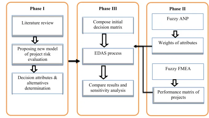
The proposed model to evaluate construction projects based on risk variables can be presented in 356
three phases (Figure 1): 357
Phase I - In the first phase, a team of experts will define the risk attributes, decision alternatives and 358
level of complexity. In this phase, the proposed integrated model will be explained to the experts. 359
Phase II - The second phase based on the ANP principles represents the relationship and interaction 360
among the decision variables and constructs the pairwise comparison matrix (shown in Figure 2). The 361
fuzzy ANP utilizes this matrix to estimate weights of the decision factors and sub-factors. Further in 362
this phase, the initial risk matrix for alternative projects is decided through a new fuzzy FMEA scoring,. 363
Three decision makers (DMs) present their views over projects considering risk determination values. 364
The fuzzy FMEA procedure is explained earlier in the paper. The outputs of this phase will be the input 365
(weights of the attributes and performance rating of projects) of phase III. 366
367
<< Insert Figure 1 about here >> 368
369
Phase III - At last, in the third phase, the EDAS method (as described earlier) evaluates projects and 370
ranks them from the best to worst. Comparisons with other MCDM methods and sensitivity analysis 371
are performed in order to test the consistency and stability of the results. 372
373
Implementation of the proposed approach 374
In this section, the implementation process of the proposed approach is discussed. Six projects 375
considered in this study are medium to large scale construction projects. These projects are related to 376
building water reservoirs and dams in one of the European countries. Due to the lack of rain and 377
decreasing water resources, the need to construct water reservoirs and dams to improve water 378
availability for agriculture is one of the important issues in this country. All of these projects are from 379
different regions of the country with varying degree of resources availability, weather conditions, 380
geographical features and political situations. Assessing and measuring the risks in developing these 381
construction projects are vital for the successful completion of the projects. Also for planning purpose, 382
it is important to understand the risks involved due to limited resources available for these projects. 383
The risk evaluation of these construction projects in this study is based on measuring the risks with the 384
help of the proposed decision analysis model and then rate them according to different risk parameters. 385
The proposed approach is implemented in consultation with the practitioners and planners to 386
<< Insert Figure 2 about here >> 389
390
Phase I - This study examines the hierarchical risk breakdown structure (RBS) for risk assessment of 391
construction projects. Organizations use RBS in conjunction with Work Breakdown Structure (WBS) 392
to help management team and eventually analyze risks (Mantel et al. 2011). For the six construction 393
projects, specific risks must be identified and analyzed. In this phase, ANP tool is used to produce the 394
weights of risk factors and sub factors. ANP is an applied tool in MCDM which considers the inter-395
relationship among risk elements using pairwise comparison. The ANP network (Figure 2) presents 396
the criteria and sub-criteria for the risk assessment of the construction projects. Different decision 397
variables for risk evaluation in construction projects are identified based on past literature such as 398
Antuchevičiene et al. (2010) and Zavadskas et al. 2010). However, these factors and sub-factors are 399
later verified during the interviews with the key decision makers in the construction projects. The risk 400
factors in this study are classified into three groups : a) Technical, b) External and c) internal / 401
organisational risk factors. The technical factors include: C1) construction requirements; C2) 402
technology; C3) complexity and interfaces; C4) quality and C5) cost; external factors include C6) 403
subcontractors and suppliers; C7) economic and market; C8) weather; and C9) political; and internal 404
factors include C10) resources; C11) funding; and C12) project site. 405
Later on, the pairwise comparisons among different decision factors and sub-factors are performed, 406
which help to get global weighs of each factors and sub-factors to decide the final risk assessment of 407
the projects. The project risk ratings are determined using fuzzy linguistic variables. 408
409
Phase II - In order to obtain the weights of factors and sub-factors using ANP, the pairwise comparison 410
matrix must be performed between factors and sub-factors. To shape the global weight matrix for all 411
the factors, primarily pairwise comparison must be made between each factor and sub-factors based 412
on the defined inter-dependency. 413
For the FMEA process, three experts / decision makers (DM) deliver their judgments for six projects 414
regarding each decision variable. These decision makers were selected based on their wide experience 415
in manging large scale construction projects. The decision makers selected for this study for providing 416
pairwise comparison of different risk factors and sub-factors have more than 20 years of working 417
experience. Appendix 1 shows the fuzzy FMEA pre-defined values (FMEA reference rating scales). 418
In this phase the experts carefully consider probability, severity and number of detection parameters 419
using fuzzy linguistic variables. For example DM1 explains for project 1 corresponding C2 the severity 420
(S), probability of happening (O) and detection are (1,1,3), (3,5,7) and (1,1,3), respectively. Appendix 421
2 presents the information of projects expressed by decision experts. Then linguistic variables are 422
translated to fuzzy values and also the defuzzification process is established. 423
424
With the help of the decision makers, pairwise comparisons are performed for the three factors to find 425
independent weights of factors (shown in Table 3). To design Table 3, experts are asked to compare 426
three factors to realize their influence. This task is done using reference scales in Table 1. After that 427
comparison between each factor is performed with regard to the single factor. Table 3 is developed 428
based on the experts’ judgment over the importance of different risk factors. For example, as the 429
external factors were identified 5 times more important than technical factors. Therefore, the priority 430
of technical factors over external are 0.2 times. After the pair wise comparison of each factor, sum of 431
each column is obtained. Then, each element is divided by the sum of the column. Finally, average of 432
each raw produces the weights which are seen in the last column. Similar process is followed for each 433
pairwise matrix of the decision variables. 434
435
<< Insert Table 3 about here >> 436
In ANP, when decision system contains factors and sub-factors, pairwise comparisons must be 438
performed in order to find importance (weight) of one over another. The weight of different factors are 439
obtained through multiplication of factors inter-dependence vector and the vector of factors 440
interrelationship with respect to each one. As there are three key decision factors ( Technical, External, 441
and Internal) in this study, four vectors (one for inter dependence and one each for three factors) should 442
be multiplied to calculate the final weight of the factor (as shown in equation 24). 443 𝑤3456789 = ;0.667 0.245 0.5250.15 0.428 0.334 0.183 0.327 0.142 F × ;0.1020.686 0.211 F = ;0.3470.38 0.273 F (24) 444 445
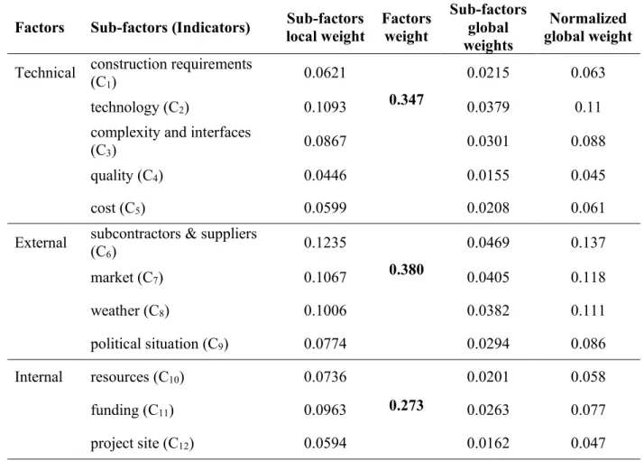
Similarly, the pair-wise comparison of 12 sub-factors are performed to find the local-weight of each 446
sub-factor. It is then multiplied to the weight of the corresponding risk factor ( Technical, External, or 447
Internal - as calculated in equation 24) to generate the global weights of each sub-factors. Finally, the 448
normalised weights of each factor are presented in Table 4. The normalized global weights of sub-449
factors are utilized in the project evaluation process by EDAS in Phase III. EDAS needs the weights 450
of decision factors and sub-factors to find the final ranking of the projects. 451
<< Insert Table 4 about here >> 452
453 454
Phase III - This section ranks projects using the EDAS method. The aggregated defuzzified matrix 455
(Appendix 3) is used as the initial decision matrix for the EDAS method. The process of ranking 456
alternative projects using EDAS first involves developing the positive distance from average (PDA) 457
and negative distance from average (NDA) matrices as described in equation 17 and 18 (See Appendix 458
4). Then, the weighted summation of the positive distance (SP) and negative distance (SN) from the 459
average matrix are obtained (as shown in equation 19 and 20). Further, the normalised values of SP 460
and SN for all alternatives (NSP and NSN) are calculated. Finally the appraisal scores (AS) of each 461
alternative are computed according to equation 23. The project with highest appraisal score is 462
considered as the riskiest project. The summary results obtained by the EDAS method and the ranking 463
of the projects are presented in Table 5. 464
<< Insert Table 5 about here >> 465
466
The ranking of projects based on EDAS shows this arrangement: 467
Project 4 > Project 6 > Project 1> Project 3> Project 5 > Project 2 468
Therefore, it is observed that project 4 is the riskiest project based on the judgments of experts and 469
corresponding risk factors. Project 2 is considered as the least risky project among all. It is observed 470
Appendix 3), that Project 4 has the maximum value regarding the criteria “subcontractors and 471
suppliers” (C6) which is the most important criterion among all. Also, this project has considered as 472
one of the low cost project among others. The results are confirmed through observing the initial data. 473
In this phase, to check the consistency and the accuracy of the obtained ranking outcomes, a 474
comparison of the proposed approach with other popular methods is conducted. EDAS ranking scores 475
are compared with other MCDM tools such as SAW, TOPSIS, VIKOR, COPRAS and WASPAS. The 476
consistency of the proposed method is evident among the ranking orders of the different methods. 477
Table 6 shows the comparative results, and tests the stability of the model. 478
479 480
<< Insert Table 6 about here >> 481
482 483
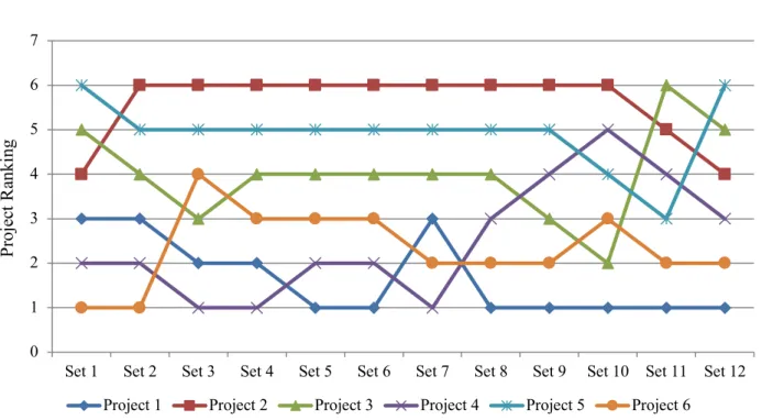
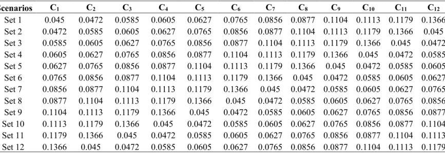
Further, sensitivity analysis is conducted on the decision parameters to study the changes in the ranking 484
of the projects. To conduct the sensitivity analysis, relative preferences of experts over the risk factors 485
and sub-factors are altered and weights of decision variables are replaced by random weights. The 486
performance of proposed approach has been then compared and analyzed for each scenario. Each 487
generated to analyze the impact on project ranking (as shown in figure 3). Table 7 shows the weight 489
replacement scenarios for six projects with respect to the decision variables. Figure 3 shows that 490
significant changes were observed in the ranking orders of the projects. Based on the sensitivity 491
analysis outcomes, it could be concluded that on average, Project 1, Project 4, and Project 6 are the top 492
3 riskiest projects. 493
<< Insert Table 7 about here >> 494
495
<< Insert Figure 3 about here >> 496
497
Discussion 498
The approach proposed for the risk evaluation of projects in this study embraces multi-level internal, 499
external and organizational factors. The proposed decision framework can help to provide suggestions 500
and improvements for practitioners to improve their decision making capabilities. Generally the 501
interrelationships among different levels of project evaluation are not considered by project managers. 502
This partially blocks the decision-making process from its most accurate route and enhances the 503
complexity of the computations. This paper essentially insists on the importance of taking into 504
consideration such interrelationships and shows how it can be done though utilizing ANP. The 505
proposed approach offers the additional opportunity for practitioners to express their comparisons 506
using fuzzy linguistic values with ANP. 507
This paper introduces a new FMEA structure utilizing fuzzy linguistic variables. The paper argues that 508
this novel pattern offers a unique anatomy, which increases judgment’s preciseness and facilitates 509
efficient decision-making procedure. The FMEA rating classification easily converts solid fuzzy values 510
to the meaningful and informative codes that are exhibited in Appendix 1. Moreover, it gives reliable 511
combination of fuzzy scales to constant alarm codes (EXH as extremely high, VH as very high). This 512
will decrease the complexity of the judging process and allow the DM to perform a better analysis of 513
the existing project. 514
515
Conclusion and future research direction 516
517
Project risk management is increasingly becoming challenging due to the number of variables and 518
parameters with quantitative and qualitative characteristics. Uncertainty and impreciseness have 519
emerged as influential factors at the core of risk evaluation computations. Mitigating complexity, 520
interrelationship and transaction among risk variables is a serious concern for project managers. In this 521
paper, a new integrated model of combining FANP and FMEA in a fuzzy decision-making 522
environment has been proposed to evaluate the potential risks of projects considering internal / 523
organizational, external and technical factors. The ANP with fuzzy linguistic scales is applied in order 524
to obtain relative weights of the sub-criteria and to resolve internal dependencies. In addition, failure 525
mode and effect analysis (FMEA) has been conducted to comprehensively measure fundamental 526
factors such as the likelihood, severity and detection of potential risk for each project. Explaining and 527
rating these factors by verbal codes is crucial. Therefore, the utilization of fuzzy linguistic scales is 528
appropriate to deal with such vagueness and uncertainty in comparing the priority of variables. The 529
proposed FMEA coding improves the decision process and increases the flexibility and efficiency of 530
risk evaluation. In this paper, decision makers offered their opinions regarding FMEA codes and then 531
through defuzzification process, the consequences assessed by them provided the main decision matrix 532
for MCDM process. The proposed framework provides a robust decision-making tool which can aid 533
project managers and investors to analyze different risk factors in multiple levels of a project. 534
The paper contributes in developing the body of knowledge in MCDM field. A new feature is the 535
integration of the EDAS method in to the risk evaluation process – something that was not considered 536
decision variables. Depending on the dimensions and levels of decision, a large pairwise comparison 538
needs to be carried out and, in such cases; fatigue is a serious concern that may cause some reliability 539
issues. In this situation, involving more decision makers in the research could be advantageous. 540
The proposed integrated MCDM model for risk evaluation can be applied to other decision-making 541
problems such as supply chain risk assessment, productivity and ergonomic risk evaluation in human 542
resource management studies. Although, ANP is a method which analyzes the interactions among 543
decision variables, it cannot recognize the direction of that interaction. In order to tackle that 544
shortcoming future research could expand the scope of this study by addressing the inter-relationships 545
among the criteria using Decision Making Trial and Evaluation Laboratory (DEMATEL) or 546
interpretive structural modeling (ISM) (Hashemi et al. 2015). Another potential improvement in the 547
project evaluation exercise could be the consideration of the risk of investment and, the satisfaction of 548
stakeholders and external customers. Integration of MCDM methods with Quality Function 549
Deployment (QFD) could be considered in future research to address this issue. Moreover, due to the 550
increasing awareness of environmental and social issues, incorporating ecological and sustainability 551
factors in the risk measurement model could be included in the proposed model. 552
553
Data Availability Statement 554
Data generated or analyzed during the study are available from the corresponding author by request. 555
References 556
Abdi, M.R.(2009). Fuzzy multi-criteria decision model for evaluating reconfigurable machines, 557
International Journal of Production Economics, 117(1), 1–15. 558
Abdi, M.R. and Labib, A.W. (2004). Feasibility study on the tactical-design justification of 559
Reconfigurable Manufacturing Systems (RMSs) using fuzzy AHP, International Journal of 560
Production Research, 42(15), 3055-3076. 561
Abdelgawad, M., & Fayek, A. R. (2010). Risk management in the construction industry using 562
combined fuzzy FMEA and fuzzy AHP. Journal of Construction Engineering and 563
Management, 136(9), 1028-1036. 564
Andery, P. R., Vanni, C., & Borges, G. (2000). Failure Analysis Applied To Design Optimisation. 565
In the proceedings of the Annual Conference Of International Group For Lean 566
Construction (Vol. 8). 567
Antuchevičiene, J., Zavadskas, E. K., & Zakarevičius, A. (2010). Multiple criteria construction 568
management decisions considering relations between criteria. Technological and Economic 569
Development of Economy, 16(1), 109-125. 570
Akintoye, A. S., & MacLeod, M. J. (1997). Risk analysis and management in construction. 571
International Journal of project management, 15(1), 31-38. 572
Chan, A. P., Scott, D., & Chan, A. P. (2004). Factors affecting the success of a construction project. 573
Journal of construction engineering and management, 130(1), 153-155. 574
Chan, F.T.S. and Kumar, N. (2007). Global supplier development considering risk factors using fuzzy 575
extended AHP-based approach. Omega: The International Journal of Management Science, 576
35(4) 417-431. 577
Chan, F. T.S., Kumar, N., Tiwari, M. K., Lau, H. C. W., and Choy, K. L. (2008). Global supplier 578
Chang, D.Y., 1996, Theory and methodology: application of the extent analysis method on fuzzy AHP. 581
European Journal of Operational Research, 95, 649–655 582
Chang, K. L. (2013). Combined MCDM approaches for century-old Taiwanese food firm new product 583
development project selection. British Food Journal, 115(8), 1197-1210 584
Chin, K. S., Wang, Y. M., Poon, G. K. K., & Yang, J. B. (2009). Failure mode and effects analysis 585
using a group-based evidential reasoning approach. Computers & Operations Research, 36(6), 586
1768-1779. 587
Dikmen, I., Birgonul, M. T., Anac, C., Tah, J. H. M., & Aouad, G. (2008). Learning from risks: A tool 588
for post-project risk assessment. Automation in construction, 18(1), 42-50. 589
Dinmohammadi, F., & Shafiee, M. (2013). A fuzzy-FMEA risk assessment approach for offshore wind 590
turbines. International Journal of Prognostics and Health Management, 4, 59-68. 591
Fallahpour, A., Amindoust, A., Antucheviciene, J., Yazdani, M. (2016). Nonlinear Genetic-Based 592
Model for supplier selection: A comparative study, Technological and Economic Development 593
of Economy, 22(4), 532-549 594
Franceschini, F., and Galetto, M. (2001). A new approach for evaluation of risk priorities of failure 595
modes in FMEA. International Journal of Production Research, 39(13), 2991-3002. 596
Ghorabaee, M. K., Zavadskas, E. K., Olfat, L., and Turskis, Z. (2015). Multi-Criteria Inventory 597
Classification Using a New Method of Evaluation Based on Distance from Average Solution 598
(EDAS). INFORMATICA, 26(3), 435-451. 599
Ghorabaee, M. K., Zavadskas, E. K., Amiri, M., & Turskis, Z. (2016). Extended EDAS Method for 600
Fuzzy Multi-criteria Decision-making: An Application to Supplier Selection. International 601
Journal of Computers Communications & Control, 11(3), 358-371. 602
Gu, X. and Zhu, Q., 2006. Fuzzy multi-attribute decision-making method based on eigenvector of 603
fuzzy attribute evaluation space. Decision Support Systems, 41(2), pp.400-410. 604
Hashemi, S. H., Karimi, A., & Tavana, M. (2015). An integrated green supplier selection approach 605
with analytic network process and improved Grey relational analysis. International Journal of 606
Production Economics, 159, 178-191. 607
He, Q., Luo, L., Hu, Y. and Chan, A.P. (2015). Measuring the complexity of mega construction projects 608
in China—A fuzzy analytic network process analysis. International Journal of Project 609
Management, 33(3), 549-563. 610
Ho, W., He, T., Lee, C. K. M., & Emrouznejad, A. (2012). Strategic logistics outsourcing: An 611
integrated QFD and fuzzy AHP approach. Expert Systems with Applications, 39(12), 10841-612
10850. 613
Hu, A. H., Hsu, C. W., Kuo, T. C., & Wu, W. C. (2009). Risk evaluation of green components to 614
hazardous substance using FMEA and FAHP. Expert Systems with Applications, 36(3), 7142-615
7147. 616
Ignatius, J., Rahman, A., Yazdani, M., Šaparauskas, J., & Haron, S. H. (2016). An integrated fuzzy 617
ANP–QFD approach for green building assessment. Journal of Civil Engineering and 618
Management, 22(4), 551-563. 619
Isaac, S., & Navon, R. (2009). Modeling building projects as a basis for change control. Automation 620
in Construction, 18(5), 656-664. 621
Kang, H. Y., Lee, A. H., & Yang, C. Y. (2012). A fuzzy ANP model for supplier selection as applied 622
to IC packaging. Journal of Intelligent Manufacturing, 23(5), 1477-1488. 623
Kerzner, H. R. (2011). Project management metrics, KPIs, and dashboards: a guide to measuring and 624
monitoring project performance. John Wiley & Sons. 625
Lavender, S. A., Mehta, J. P., & Allread, W. G. (2013). Comparisons of tibial accelerations when 626
walking on a wood composite vs. a concrete mezzanine surface. Applied ergonomics, 44(5), 824-627
Liu, H. C., Liu, L., Liu, N., & Mao, L. X. (2012). Risk evaluation in failure mode and effects analysis 629
with extended VIKOR method under fuzzy environment. Expert Systems with 630
Applications, 39(17), 12926-12934. 631
Liu, H. C., Liu, L., & Liu, N. (2013). Risk evaluation approaches in failure mode and effects analysis: 632
A literature review. Expert Systems with Applications, 40(2), 828–838. 633
Lowe, D. (2013) Commercial Management: Theory and Practice, John Wiley & Sons. 634
Mantel Jr, S. J., Meredith, J. R., Shafer, S. M., & Sutton, M. M. (2001). Project management in practice. 635
Wiley. 636
Maytorena, E., Winch, G. M., Freeman, J., & Kiely, T. (2007). The influence of experience and 637
information search styles on project risk identification performance. IEEE Transactions on 638
Engineering Management, 54(2), 315-326 639
Nielsen, A. (2002). Failure modes and effects analysis (FMEA) used on moisture problems. Indoor 640
Air, 38-43. 641
Peng, X., and Selvachandran, G. (2017). Pythagorean fuzzy set: state of the art and future directions, 642
Artificial Intelligence Review, 1-55. 643
Prakash, C., and Barua, M. K. (2016). A combined MCDM approach for evaluation and selection of 644
third-party reverse logistics partner for Indian electronics industry. Sustainable Production and 645
Consumption, 7, 66-78. 646
Saaty, T. L. (1980). The analytic hierarchy process: planning, priority setting, resources allocation. 647
New York: McGraw. 648
Saaty, T. L. (1996). Multi-criteria decision making. The Analytic Hierarchy Process, Pittsburgh. 649
Safari, H., Faraji, Z., & Majidian, S. (2016). Identifying and evaluating enterprise architecture risks 650
using FMEA and fuzzy VIKOR. Journal of Intelligent Manufacturing, 27(2), 475-486. 651
Sharma, R. K., Kumar, D., & Kumar, P. (2005). Systematic failure mode effect analysis (FMEA) using 652
fuzzy linguistic modelling. International Journal of Quality & Reliability Management, 22(9), 653
986-1004. 654
Shyur, H. J. (2006). COTS evaluation using modified TOPSIS and ANP. Applied mathematics and 655
computation, 177(1), 251-259. 656
Tadić, S., Zečević, S., & Krstić, M. (2014). A novel hybrid MCDM model based on fuzzy DEMATEL, 657
fuzzy ANP and fuzzy VIKOR for city logistics concept selection. Expert Systems with 658
Applications, 41(18), 8112-8128. 659
Tavana, M., Yazdani, M., & Di Caprio, D. (2016). An application of an integrated ANP–QFD 660
framework for sustainable supplier selection. International Journal of Logistics Research and 661
Applications, 1-22. 662
Tsaur, S. H., and Wang, C. H. (2007). The evaluation of sustainable tourism development by analytic 663
hierarchy process and fuzzy set theory: An empirical study on the Green Island in Taiwan. Asia 664
Pacific Journal of Tourism Research, 12 (2), 127-145. 665
Tserng, H. P., Yin, S. Y., Dzeng, R. J., Wou, B., Tsai, M. D., & Chen, W. Y. (2009). A study of 666
ontology-based risk management framework of construction projects through project life cycle. 667
Automation in Construction, 18(7), 994-1008. 668
Tzeng, G. H., Chiang, C. H., & Li, C. W. (2007). Evaluating intertwined effects in e-learning programs: 669
A novel hybrid MCDM model based on factor analysis and DEMATEL. Expert systems with 670
Applications, 32(4), 1028-1044. 671
Wang, Y. M., Chin, K. S., Poon, G. K. K., & Yang, J. B. (2009). Risk evaluation in failure mode and 672
effects analysis using fuzzy weighted geometric mean. Expert systems with applications, 36(2), 673
1195-1207. 674
Wheeler, D.J. 2011, Problems With Risk Priority Numbers, Quality Digest, available at : 675 https://www.qualitydigest.com/inside/quality-insider-column/problems-risk-priority-676 numbers.html 677
Yang, J. L., and Tzeng, G. H. (2011). An integrated MCDM technique combined with DEMATEL for 678
a novel cluster-weighted with ANP method. Expert Systems with Applications, 38(3), 1417-679
1424. 680
Yazdani, M. and Payam, A. F. (2015). A comparative study on material selection of 681
microelectromechanical systems electrostatic actuators using Ashby, VIKOR and 682
TOPSIS. Materials & Design, 65, 328-334. 683
Yazdani, M., Hashemkhani Zolfani, S., and Zavadskas, E. K. (2016). New integration of MCDM 684
methods and QFD in the selection of green suppliers. Journal of Business Economics and 685
Management, 1-17. 686
Zadeh, L. A. (1965). Fuzzy sets. Information and control, 8(3), 338-353. 687
Zavadskas, E. K., Turskis, Z. and Tamošaitiene, J. (2010). Risk assessment of construction projects. 688
Journal of civil engineering and management, 16(1), 33-46. 689
Zwikael, O., & Globerson, S. (2006). Benchmarking of project planning and success in selected 690
industries. Benchmarking: An International Journal, 13(6), 688-700. 691
List of Figures 693
694 695
Figure 1. Three phase MCDM model for project risk evaluation problem 696
Figure 2. Risk factors and sub-factors relationship and network diagram for ANP 697
Figure 3. EDAS ranking outcomes based on different scenarios of sensitivity analysis 698
699 700 701 702 703 704 705 706 707 708 709 710 711 712 713 714 715
Figure 1. Three phase MCDM model for project risk evaluation problem 716
717 718
Phase I Phase III Phase II
Literature review
Proposing new model of project risk
evaluation
Decision attributes & alternatives determination Fuzzy ANP Weights of attributes Fuzzy FMEA Performance matrix of projects EDAS process
Compare results and sensitivity analysis
Compose initial decision matrix
719
720
Figure 2. Risk factors and sub-factors relationship and network diagram for ANP 721
723 724 725
726 727
Figure 3. EDAS ranking outcomes based on different scenarios of sensitivity analysis 728 729 0 1 2 3 4 5 6 7
Set 1 Set 2 Set 3 Set 4 Set 5 Set 6 Set 7 Set 8 Set 9 Set 10 Set 11 Set 12 Project 1 Project 2 Project 3 Project 4 Project 5 Project 6
P roj ec t R anki ng
730
Table 1. Fuzzy scale for pairwise comparisons 731
732
Fuzzy number Linguistic variables Triangular fuzzy number
9I Extremely important/preferred (7,9,9)
7I Very strongly important/preferred (5,7,9)
5I Strongly important/preferred (3,5,7)
3I Moderately important/preferred (1,3,5)
1I Equally important/preferred (1,1,3)
734
Table 2. Classification of fuzzy linguistic variables for RPN scoring 735 736 Linguistic Term Fuzzy Number
Severity Occurrence Detection
Very Low A failure that has no/ minor effect on the system performance, the operator probably will not notice.
It would be very unlikely for these failures to be observed.
Defect remains undetected until the system performance degrades to the extent that the task will not be completed.
Low A failure that would cause
slight annoyance to the operator, but that cause no deterioration to the system.
Likely to occur
once, but
unlikely to occur more frequently.
Defect remains undetected until system performance is severely reduced.
Medium A failure that would cause a high degree of operator dissatisfaction or that causes noticeable but slight deterioration in system performance.
Likely to occur more than once.
Defect remains undetected until system performance is affected.
High A failure that causes
significant deterioration in system performance and/or leads to minor injuries.
Near certain to occur at least once.
Defect remains undetected until an inspection/test is carried out.
Very High A failure that would seriously affect the ability to complete The task or cause damage, serious injury or death.
Almost certain to occur several times.
Failure remains undetected, until a full inspection and test is completed. 737 738 739 740 ^ 1 ^ 3 ^ 5 ^ 7 ^ 9
741
Table 3. Pairwise comparison matrix for decision variables 742
Comparative rating of all factors
Factors Technical External Internal weight Technical 1 0.2 0.33 0.1111 0.1429 0.0526 0.102
External 5 1 5 0.5556 0.7143 0.7895 0.686
Internal 3 0.2 1 0.3333 0.1429 0.1579 0.211
9 1.4 6.3
Relative importance of all factors with respect to technical factor
Technical Technical External Internal weight
Technical 1 3 7 0.6774 0.5 0.8235 0.667
External 0.33 1 0.5 0.2258 0.1667 0.0588 0.150 Internal 0.14 2 1 0.0968 0.3333 0.1176 0.183
1.48 6 8.5
Relative importance of all factors with respect to external factor
External Technical External Internal weight Technical 1 0.14 2 0.1176 0.0455 0.5714 0.245
External 7 1 0.5 0.8235 0.3182 0.1429 0.428 Internal 0.5 2 1 0.0588 0.6364 0.2857 0.327
8.5 3.1 3.5
Relative importance of all factors with respect to internal factor
Internal Technical External Internal weight
Technical 1 2 3 0.5455 0.6 0.4286 0.525
External 0.5 1 3 0.2727 0.3 0.4286 0.334
Internal 0.33 0.33 1 0.1818 0.1 0.1429 0.142
743 744 745 746
Table 4. ANP global weights assigned for each sub-factors 747
748
Factors Sub-factors (Indicators) local weight Sub-factors Factors weight
Sub-factors global weights
Normalized global weight Technical construction requirements (C
1) 0.0621
0.347
0.0215 0.063
technology (C2) 0.1093 0.0379 0.11
complexity and interfaces
(C3) 0.0867 0.0301 0.088
quality (C4) 0.0446 0.0155 0.045
cost (C5) 0.0599 0.0208 0.061
External subcontractors & suppliers (C
6) 0.1235 0.380 0.0469 0.137 market (C7) 0.1067 0.0405 0.118 weather (C8) 0.1006 0.0382 0.111 political situation (C9) 0.0774 0.0294 0.086 Internal resources (C10) 0.0736 0.273 0.0201 0.058 funding (C11) 0.0963 0.0263 0.077 project site (C12) 0.0594 0.0162 0.047 749 750
Table 5. Ranking of projects based on EDAS method 751 SP SN NSP NSN AS RANK Project 1 0.514 0.366 0.891 0.477 0.684 3 Project 2 0.200 0.699 0.347 0 0.174 6 Project 3 0.317 0.377 0.549 0.461 0.505 4 Project 4 0.576 0.294 1 0.580 0.790 1 Project 5 0.320 0.406 0.555 0.420 0.487 5 Project 6 0.525 0.310 0.911 0.557 0.734 2 752
Table 6. Comparison of other MCDM techniques with EDAS 753
SAW WASPAS COPRAS TOPSIS VIKOR EDAS
Project 1 3 3 3 3 4 3 Project 2 6 6 6 6 6 6 Project 3 4 4 4 5 5 4 Project 4 1 1 1 1 1 1 Project 5 5 5 5 4 3 5 Project 6 2 2 2 2 2 2 754
Table 7. Twelve scenarios for sensitivity analysis 755 Scenarios C1 C2 C3 C4 C5 C6 C7 C8 C9 C10 C11 C12 Set 1 0.045 0.0472 0.0585 0.0605 0.0627 0.0765 0.0856 0.0877 0.1104 0.1113 0.1179 0.1366 Set 2 0.0472 0.0585 0.0605 0.0627 0.0765 0.0856 0.0877 0.1104 0.1113 0.1179 0.1366 0.045 Set 3 0.0585 0.0605 0.0627 0.0765 0.0856 0.0877 0.1104 0.1113 0.1179 0.1366 0.045 0.0472 Set 4 0.0605 0.0627 0.0765 0.0856 0.0877 0.1104 0.1113 0.1179 0.1366 0.045 0.0472 0.0585 Set 5 0.0627 0.0765 0.0856 0.0877 0.1104 0.1113 0.1179 0.1366 0.045 0.0472 0.0585 0.0605 Set 6 0.0765 0.0856 0.0877 0.1104 0.1113 0.1179 0.1366 0.045 0.0472 0.0585 0.0605 0.0627 Set 7 0.0856 0.0877 0.1104 0.1113 0.1179 0.1366 0.045 0.0472 0.0585 0.0605 0.0627 0.0765 Set 8 0.0877 0.1104 0.1113 0.1179 0.1366 0.045 0.0472 0.0585 0.0605 0.0627 0.0765 0.0856 Set 9 0.1104 0.1113 0.1179 0.1366 0.045 0.0472 0.0585 0.0605 0.0627 0.0765 0.0856 0.0877 Set 10 0.1113 0.1179 0.1366 0.045 0.0472 0.0585 0.0605 0.0627 0.0765 0.0856 0.0877 0.1104 Set 11 0.1179 0.1366 0.045 0.0472 0.0585 0.0605 0.0627 0.0765 0.0856 0.0877 0.1104 0.1113 Set 12 0.1366 0.045 0.0472 0.0585 0.0605 0.0627 0.0765 0.0856 0.0877 0.1104 0.1113 0.1179 756 757 758 759