Sparse Dimensionality Reduction Methods: Algorithms and Applications

(1)

SPARSE DIMENSIONALITY REDUCTION

METHODS: ALGORITHMS AND

APPLICATIONS

ZHANG XIAOWEI

(B.Sc., ECNU, China)

A THESIS SUBMITTED

FOR THE DEGREE OF DOCTOR OF PHILOSOPHY

DEPARTMENT OF MATHEMATICS

NATIONAL UNIVERSITY OF SINGAPORE

JULY 2013

(2)

(3)

(4)

I hereby declare that the thesis is my original work and it has been written by me in its entirety. I have duly acknowledged all the sources of information which have been used in the thesis.

This thesis has also not been submitted for any degree in any university previously.

Zhang Xiaowei July 2013

(5)

Acknowledgements

First and foremost I would like to express my deepest gratitude to my supervisor, As-sociate Professor Chu Delin, for all his guidance, support, kindness and enthusiasm over the past five years of my graduate study at National University of Singapore. It is an invaluable privilege to have had the opportunity to work with him and learn many wonderful mathematical insights from him. Back in 2008 when I arrived at National University of Singapore, I knew little about the area of data mining and machine learning. It is Dr. Chu who guided me into these research areas and en-couraged me to explore various ideas, and patiently helped me improve how I do research. It would not have been possible to complete this doctoral thesis without his support. Beyond being an energetic and insightful researcher, he also helped me a lot on how to communicate with other people. I feel very fortunate to be advised by Dr. Chu.

I would like to thank Professor Li-Zhi Liao and Professor Michael K. Ng, both from Hong Kong Baptist University, for their assistance and support in my research. Interactions with them were very constructive and helped me a lot in writing this thesis.

I am greatly indebted to National University of Singapore for providing me a full scholarship and an exceptional study environment. I would also like to thank

(6)

Department of Mathematics for providing financial support for my attendance of IMECS 2013 in Hong Kong and ICML 2013 in Atlanta. The Centre for Computa-tional Science and Engineering provides large-scale computing facilities which enable me to conduct numerical experiments in my thesis.

I am also grateful to all friends and collaborators. Special thanks go to Wang Xiaoyan and Goh Siong Thye, with whom I closely worked and collaborated. With Xiaoyan, I shared all experience as a graduate student and it was enjoyable to discuss research problems or just chat about everyday life. Siong Thye is an optimistic man and taught me a lot about machine learning, and I am more than happy to see that he continues his research at MIT and is working to become the next expert in his field.

Last but not least, I want to warmly thank my family, my parents, brother and sister, who encouraged me to pursue my passion and supported my study in every possible way over the past five years.

(7)

Summary

This thesis focuses on sparse dimensionality reduction methods, which aim to find optimal mappings to project high-dimensional data into low-dimensional spaces and at the same time incorporate sparsity into the mappings. These methods have many applications, including bioinformatics, text processing and computer vision.

One challenge posed by high dimensionality is that, with increasing dimension-ality, many existing data mining algorithms usually become computationally in-tractable. Moreover, a lot of samples are required when performing data mining techniques on high-dimensional data so that information extracted from the data is accurate, which is well known as the curse of dimensionality. To deal with this

problem, many significant dimensionality reduction methods have been proposed. However, one major limitation of these dimensionality reduction techniques is that mappings learned from the training data lack sparsity, which usually makes in-terpretation of the results challenging or computation of the projections of new data time-consuming. In this thesis, we address the problem of deriving sparse version of some widely used dimensionality reduction methods, specifically, Linear Discriminant Analysis (LDA), Canonical Correlation Analysis (CCA) and its kernel extension Kernel Canonical Correlation Analysis (kernel CCA).

(12)

First, we study uncorrelated LDA (ULDA) and obtain an explicit characteriza-tion of all solucharacteriza-tions of ULDA. Based on the characterizacharacteriza-tion, we propose a novel sparse LDA algorithm. The main idea of our algorithm is to select the sparsest solution from the solution set, which is accomplished by minimizing `1-norm

sub-ject to a linear constraint. The resulted `1-norm minimization problem is solved by

(accelerated) linearized Bregman iterative method. With similar idea, we investi-gate sparse CCA and propose a new sparse CCA algorithm. Besides that, we also obtain a theoretical result showing that ULDA is a special case of CCA. Numerical results with synthetic and real-world data sets validate the efficiency of the proposed methods, and comparison with existing state-of-the-art algorithms shows that our algorithms are competitive.

Beyond linear dimensionality reduction methods, we also investigate sparse ker-nel CCA, a nonlinear variant of CCA. By using the explicit characterization of all solutions of CCA, we establish a relationship between (kernel) CCA and least squares problems. This relationship is further utilized to design a sparse kernel CCA algorithm, where we penalize the least squares term by `1-norm of the dual

transformations. The resulted`1-norm regularized least squares problems are solved by fixed-point continuation method. The efficiency of the proposed algorithm for sparse kernel CCA is evaluated on cross-language document retrieval and content-based image retrieval.

(13)

List of Tables

1.1 Sample size required to ensure that the relative mean squared error at zero is less than 0.1 for the estimate of a normal distribution . . . 3

2.1 Simulation results. The reported values are means (and standard deviations), computed over 100 replications, of classification accuracy, sparsity, orthogonality and total number of selected features. . . 37

2.2 Data stuctures: data dimension (d), training size (n), the number of classes (K) and the number of testing data (# Testing). . . 39

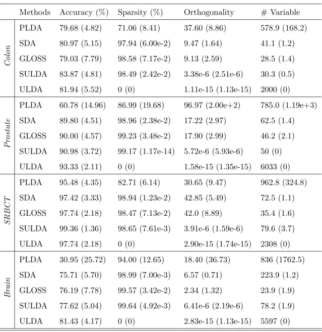
2.3 Numerical results for gene data over 10 training-testing splits: mean (and standard deviation) of classification accuracy, sparsity, orthog-onality and the number of selected variables. . . 40

2.4 Numerical results for image data over 10 training-testing splits: mean (and standard deviation) of classification accuracy, sparsity, orthog-onality and the number of selected variables. . . 41

4.1 Comparison of results obtained by SCCA `1 with µx = µy = µ and

1 =2 = 10−5, PMD, CCA EN, and SCCA PD. . . 87

(14)

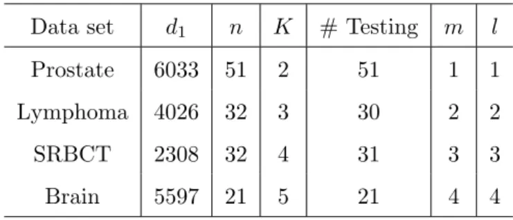
4.2 Data stuctures: data dimension (d1), training size (n), the number

of classes (K) and the number of testing data (# Testing), m is the rank of matrix XYT, l is the number of columns in Wx and Wy and

we choose l=m in our experiments. . . 88

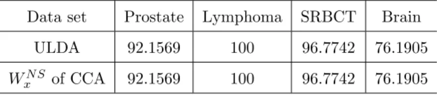
4.3 Comparison of classification accuracy (%) between ULDA and W_xN S

of CCA using 1NN as classifier . . . 89

4.4 Comparison of results obtained by SCCA `1, PMD, CCA EN, and

SCCA PD.. . . 90

4.5 Comparison of results obtained by SCCA `1, PMD, CCA EN, and

SCCA PD.. . . 91

4.6 Average AROC of standard CCA and sparse CCA algorithms using Data Set I (French to English). . . 97

4.7 Average AROC of standard CCA, SCCA `1 and SCCA PD using

Data Set II (French to English). . . 98

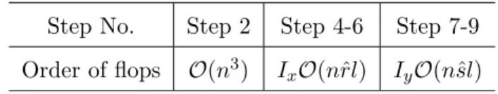
5.1 Computational complexity of Algorithm 7 . . . 120

5.2 Correlation between the first pair of canonical variables obtained by ordinary CCA, RKCCA and SKCCA. . . 121

5.3 Cross-language document retrieval using CCA, KCCA, RKCCA and SKCCA. . . 125

(15)

List of Figures

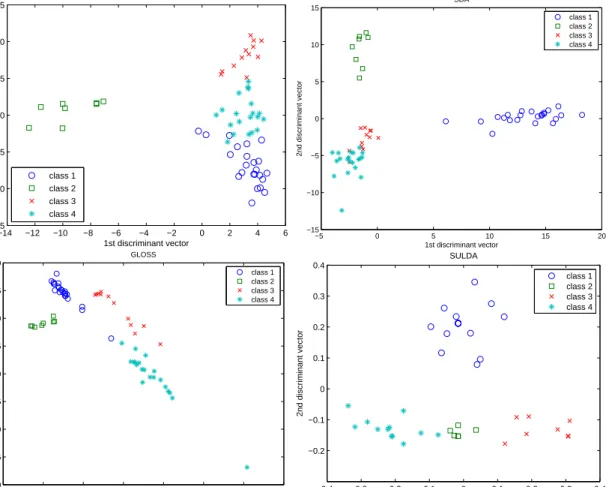
2.1 2D visualization of the SRBCT data: all samples are projected onto the first two sparse discriminant vectors obtained by PLDA (upper left), SDA (upper right), GLOSS (lower left) and SULDA (lower right), respectively. . . 42

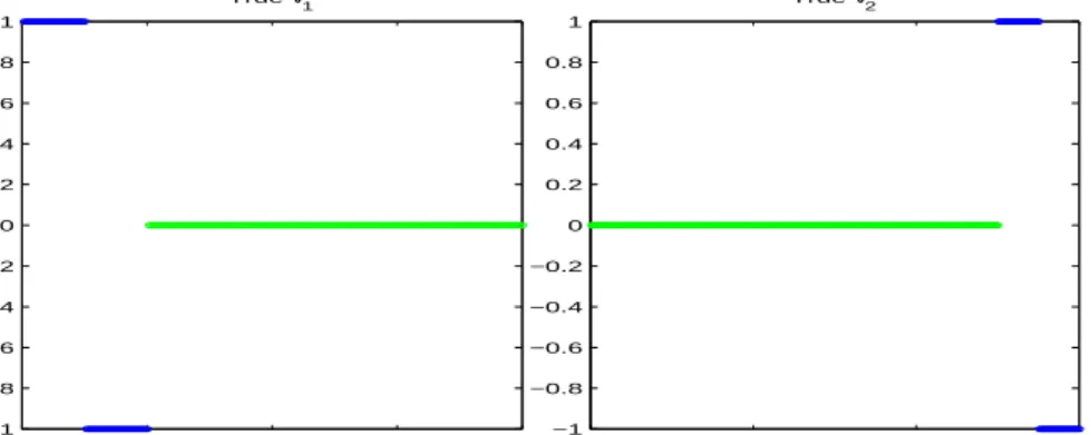
4.1 True value of vectorsv1 and v2. . . 85

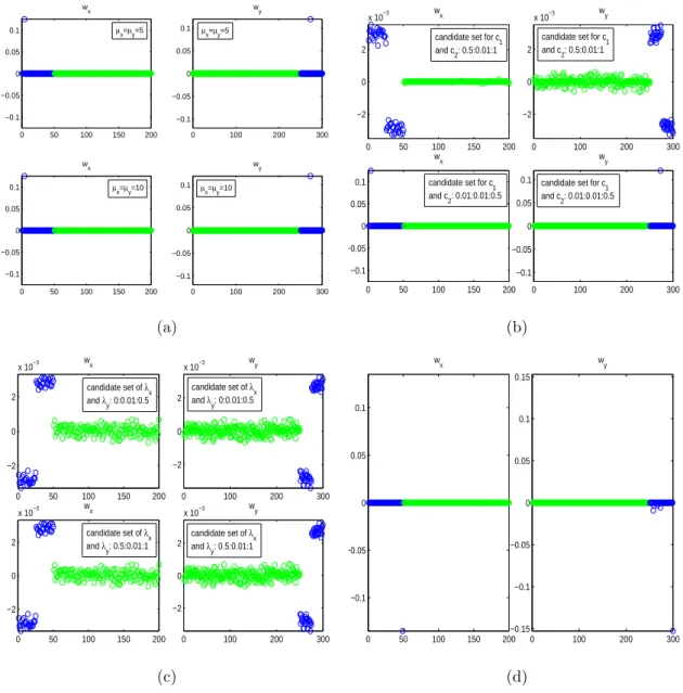
4.2 WxandWycomputed by different sparse CCA algorithms: (a) SCCA `1

(our approach), (b) Algorithm PMD, (c) Algorithm CCA EN, (d) Al-gorithm SCCA PD. . . 86

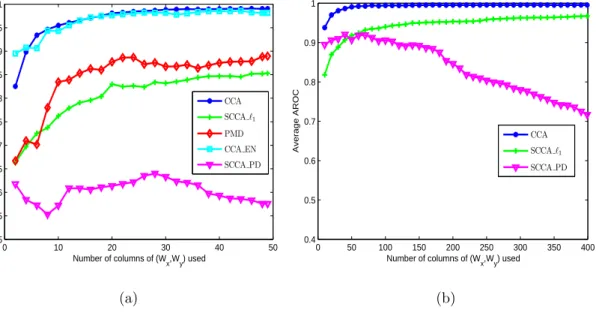
4.3 Average AROC achieved by CCA and sparse CCA as a function of the number of columns of (Wx, Wy) used: (a) Data Set I, (b) Data

Set II. . . 96

5.1 Plots of the first pair of canonical variates:(a) sample data, (b) ordi-nary CCA, (c) RKCCA, (d) SKCCA. . . 122

(16)

5.2 Cross-language document retrieval using CCA, KCCA, RKCCA and SKCCA: (a) Europarl data with 50 training data, (b) Europarl data with 100 training data,(c) Hansard data with 200 training data, (d) Hansard data with 400 training data. . . 124

5.3 Gabor filters used to extract texture features. Four frequencies f = 1/λ = [0.15,0.2,0.25,0.3] and four directions θ = [0, π/4, π/2,3π/4] are used. The width of the filters areσ = 4. . . 128

5.4 Content-based image retrieval using CCA, KCCA, RKCCA and SKCCA on UW ground truth data with 217 training data. . . 130

(17)

Chapter

1

Introduction

Over the past few decades, data collection and storage capabilities as well as data management techniques have achieved great advances. Such advances have led to a leap of information in most scientific and engineering fields. One of the most sig-nificant reflections is the prevalence of high-dimensional data, including microarray gene expression data [7,51], text documents [12,90], functional magnetic resonance imaging (fMRI) data [59, 154], image/video data and high-frequency financial data, where the number of features can reach tens of thousands. While the proliferation of high-dimensional data lays the foundation for knowledge discovery and pattern anal-ysis, it also imposes challenges on researchers and practitioners of effectively utilizing these data and mining useful information from them, due to the high dimensionality character of these data [47]. One common challenge posed by high dimensionality is that, with increasing dimensionality, many existing data mining algorithms usually become computationally intractable and therefore inapplicable in many real-world applications. Moreover, a lot of samples are required when performing data mining techniques on high-dimensional data so that information extracted from the data is accurate, which is well known as the curse of dimensionality.

(18)

1.1 Curse of Dimensionality

The phrase ‘curse of dimensionality’, apparently coined by Richard Bellman in [117], is used by the statistical community to describe the problem that the number of samples required to estimate a function with a specific level of accuracy grows expo-nentially with the dimension it comprises. Intuitively, as we increase the dimension, most likely we will include more noise or outliers as well. In addition, if the samples we collect are inadequate, we might be misguided by the wrong representation of the data. For example, we might keep sampling from the tail of a distribution, as illustrated by the following example.

Example 1.1. Consider a sphere of radius r in d dimensions together with the concentric hypercube of side 2r, so that the sphere touches the hypercube at the centres of each of its sides. The volume of the hypercube is (2r)d and the volume of the sphere is 2r_dΓ(d/2)dπd/2, where Γ(·) is the gamma function defined by

Γ(x) =

Z ∞

0

ux−1e−udu.

Thus, the ratio of the volume of the sphere to the volume of the cube is given by

πd/2

d2d−1_Γ(d/2), which converges to zero as d → ∞. We can see from this result that, in

high dimensional spaces, most of the volume of a hypercube is concentrated in the

large number of corners.

Therefore, in the case of a uniform distribution in high-dimensional space, most of the probability mass is concentrated in tails. Similar behaviour can be observed for

the Gaussian distribution in high-dimensional spaces, where most of the probability mass of a Gaussian distribution is located within a thin shell at a large radius [15].

Another example illustrating the difficulty imposed by high dimensionality is kernel density estimation.

Example 1.2. Kernel density estimation (KDE) [20] is a popular method for esti-mating probability density function (PDF) for a data set. For a given set of samples

(19)

1.1 Curse of Dimensionality 3

{x1,· · · , xn} in Rd, the simplest KDE aims to estimate the PDF f(x) at a point

x∈_Rd _{with the estimation in the following form:}

ˆ fn(x) = 1 n n X i=1 1 hd n k _k x−xik hn ,

where hn = _nd1+4 is the bandwidth, k: [0,∞)→[0,∞)is a kernel function satisfying

certain conditions. Then the mean squared error in the estimate fˆn(x) is given by

M SE[ ˆfn(x)] =_E[( ˆfn(x)−f(x))2] =O 1 n4/(d+4) , as n→ ∞.

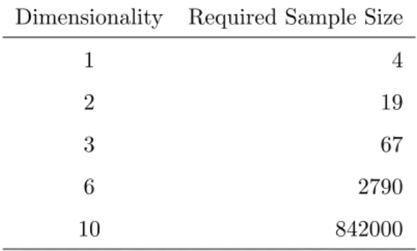
Thus, the convergence rate slows as the dimensionality increases. To achieve the same convergence rate with the case where d= 10 and n= 10,000, approximately 7 million (i.e., n ≈7×106) samples are required if the dimensionality is increased to

d = 20. To get a rough idea of the impact of sample size on the estimation error, we can look at the following table, taken from Silverman [129], which illustrates how the sample size required for a given relative mean squared error for the estimate of

a normal distribution increases with the dimensionality.

Table 1.1: Sample size required to ensure that the relative mean squared error at zero is less than 0.1 for the estimate of a normal distribution

Dimensionality Required Sample Size

1 4

2 19

3 67

6 2790

10 842000

Although the curse of dimensionality draws a gloomy picture for high-dimensional data analysis, we still have hope in the fact that, for many high-dimensional data in practice, theintrinsic dimensionality [61] of these data may be low in the sense that the minimum number of parameters required to account for the observed properties of these data is much smaller. A typical example of this kind arises in document

(20)

Example 1.3 (Text document data). The simplest possible way of representing a document is as a bag-of-words, where a document is represented by the words it

contains, with the ordering of these words being ignored. For a given collection of documents, we can get a full set of words appearing in the documents being processed.

The full set of words is referred as the dictionary whose dimensionality is typically in tens of thousands. Each document is represented as a vector in which each coordinate

describes the weight of one word from the dictionary.

Although the dictionary has high dimensionality, the vector associated with a

given document may contain only a few hundred non-zero entries, since the document typically contains only very few of the vast number of words in the dictionary. In

this sense, the intrinsic dimensionality of this data is the number of non-zero entries in the vector, which is far smaller than the dimensionality of the dictionary.

To avoid the curse of dimensionality, we can design methods which depend only on the intrinsic dimensionality of the data; or alternatively work on the low-dimensional data obtained by applying dimensionality reduction techniques to the

high-dimensional data.

1.2 Dimensionality Reduction

Dimensionality reduction, aiming at reducing the dimensionality of original data, transforms the high-dimensional data into a much lower dimensional space and at the same time preserves essential information contained in the original data as much as possible. It has been widely applied in many areas, including text mining, im-age retrieval, face recognition, handwritten digit recognition and microarray data analysis.

Besides avoiding the curse of dimensionality, there are many other motivations for us to consider dimensionality reduction. For example, dimensionality reduction can remove redundant and noisy data and avoid data over-fitting, which improves

(21)

1.2 Dimensionality Reduction 5

the quality of data and facilitates further processing tasks such as classification and retrieval. The need for dimensionality reduction also arises for data compres-sion in the sense that, by applying dimencompres-sionality reduction, the size of the data can be reduced significantly, which saves a lot storage space and reduces computa-tional cost in further processing. Another motivation of dimensionality reduction is data visualization. Since visualization of high-dimensional data is almost beyond the capacity of human beings, through dimensionality reduction, we can construct 2-dimensional or 3-dimensional representation of high-dimensional data such that essential information in the original data is preserved.

In mathematical terms, dimensionality reduction can be defined as follows. As-sume we are given a set of training data

A=ha1 · · · an

i

∈_Rd×n

consisting of n samples from d-dimensional space. The goal is to learn a mapping

f(·) from the training data by optimizing certain criterion such that, for each given data x∈_Rd_, _f₍_x_{) is a low-dimensional representation of} _x_.

The subject of dimensionality reduction is vast, and can be grouped into dif-ferent categories based on difdif-ferent criteria. For example, linear and non-linear dimensionality reduction techniques; unsupervised, supervised and semi-supervised dimensionality reduction techniques. In linear dimensionality, the function f is lin-ear, that is,

xL=f(x) = WTx, (1.1)

where W ∈ _Rd×l ₍_l _d_{) is the} _{projection matrix} _{learned from training data, e.g.,}

Principal Component Analysis (PCA) [87], Linear Discriminant Analysis (LDA) [50,56, 61] and Canonical Correlation Analysis (CCA) [2,79]. In nonlinear dimen-sionality reduction [100], the function f is non-linear, e.g., Isometric feature map (Isomap) [137], Locally Linear Embedding (LLE) [119, 121], Laplacian Eigenmaps [11] and various kernel learning techniques [123, 127]. In unsupervised learning, the training data are unlabelled and we are expected to find hidden structure of

(22)

these unlabelled data. Typical examples of this type include Principal Component Analysis (PCA) [87] and K-mean Clustering [61]. In contrast to unsupervised learn-ing, in supervised learnlearn-ing, we know the labels of training data, and try to find the discriminant function which best fits the relation between the training data and the labels. Typical examples of supervised learning techniques include Linear Discrim-inant Analysis (LDA) [50, 56, 61], Canonical Correlations Analysis (CCA) [2, 79] and Partial Least Squares (PLS) [148]. Semi-supervised learning falls between un-supervised and un-supervised learning, and makes use of both labelled and unlabelled training data (usually a small portion of labelled data with a large portion of un-labelled data). As a relatively new area, semi-supervised learning makes use of the strength of both unsupervised and supervised learning and has attracted more and more attention during last decade. More details of semi-supervised learning can be found in [26].

In this thesis, since we are interested in accounting label information for learn-ing, we restrict our attention to supervised learning. In particular, we mainly focus on Linear Discriminant Analysis (LDA), Canonical Correlation Analysis (CCA) and its kernel extension Kernel Canonical Correlation Analysis (kernel CCA). As one of the most powerful techniques for dimensionality reduction, LDA seeks an optimal linear transformation that transforms the high-dimensional data into a much lower dimensional space and at the same time maximizes class separability. To achieve maximal separability in the reduced dimensional space, the optimal linear transfor-mation should minimize the within-class distance and maximize the between-class distance simultaneously. Therefore, optimization criteria for classical LDA are gen-erally formulated as the maximization of some objective functions measuring the ratio of between-class distance and within-class distance. An optimal solution of LDA can be computed by solving a generalized eigenvalue problem [61]. LDA has been applied successfully in many applications, including microarray gene expres-sion data analysis [51, 68, 165], face recognition [10, 27, 169, 85], image retrieval [135] and document classification [80]. CCA was originally proposed in [79] and has

(23)

1.3 Sparsity and Motivations 7

become a powerful tool in multivariate analysis for finding the correlations between two sets of high-dimensional variables. It seeks a pair of linear transformations such that the projected variables in the lower-dimensional space are maximally correlated. To extend CCA to non-linear data, many researchers [1, 4, 72, 102] applied kernel trick to CCA, which results in kernel CCA. Empirical results show that kernel CCA is efficient in handling non-linear data and can successfully find non-linear relationship between two sets of variables. It has also been shown that solutions of both CCA and kernel CCA can be obtained by solving generalized eigenvalue problems [14]. Applications of CCA and kernel CCA can be found in [1, 4, 42,59, 63, 72,92, 93, 102, 134, 143, 144, 158].

1.3 Sparsity and Motivations

One major limitation of dimensionality reduction techniques considered in previ-ous section is that mappings f(·) learned from training data lack sparsity, which usually makes interpretation of the obtained results challenging or computation of the projections of new data time-consuming. For instance, in linear dimensionality reduction (1.1), low-dimensional projection xL ₌ _WT_x _{of new data point} _x _{is a}

linear combination of all features in original data x, which means all features in x

contribute to the extracted features in xL_{, thus makes it difficult to interpret} _xL_;

in kernel learning techniques, we need to evaluate the kernel function at all train-ing samples in order to compute projections of new data points due to the lack of sparsity in the dual transformation (see Chapter 5 for detailed explanation), which is computationally expensive. Sparsity is a highly desirable property both theoreti-cally and computationally as it can facilitate interpretation and visualization of the extracted feature, and a sparse solution is typically less complicated and hence has better generalization ability. In many applications such as gene expression analysis and medical diagnostics, one can even tolerate a small degradation in performance to achieve high sparsity [125].

(24)

The study of sparsity has a rich history and can be dated back to the principle of parsimony which states that the simplest explanation for unknown phenomena

should be preferred over the complicated ones in terms of what is already known. Benefiting from recent development of compressed sensing [24,25,48,49] and opti-mization with sparsity-inducing penalties [3, 142], extensive literature on the topic of sparse learning has emerged: Lasso and its generalizations [53,138,139,170,173], sparse PCA [39,40,88,128,174], matrix completion [23,116], sparse kernel learning [46,132, 140, 156], to name but a few.

A typical way of obtaining sparsity is minimizing the `1-norm of the transfor-mation matrices.1 _{The use of} _`

1-norm for sparsity has a long history [138], and

extensive study has been done to investigate the relationship between a minimal `1 -norm solution and a sparse solution [24,25,28,48,49]. In the thesis, we address the problem of incorporating sparsity into the transformation matrices of LDA, CCA and kernel CCA via `1-norm minimization or regularization.

Although many sparse LDA algorithms [34,38,101,103,105,111,126,152,157] and sparse CCA algorithms [71, 114, 145, 150, 151, 153] have been proposed, they are all sequential algorithms, that is, the sparse transformation matrix in (1.1) is computed one column by one column. These sequential algorithms are usually computationally expensive, especially when there are many columns to compute. Moreover, there does not exist effective way to determine the number of columns l

in sequential algorithms. To deal with these problems, we develop new algorithms for sparse LDA and sparse CCA in Chapter 2 and Chapter 4, respectively. Our methods compute all columns of sparse solutions at one time, and the computed sparse solutions are exact to the accuracy of specified tolerance. Recently, more and more attention has been drawn to the subject of sparse kernel approaches [15,156], such as support vector machines [123], relevance vector machine [140], sparse kernel partial least squares [46,107], sparse multiple kernel learning [132], and many others.

1_{In this thesis, unless otherwise specified, the}_`

1-norm is defined to be summation of the absolute value of all entries, for both a vector and a matrix.

(25)

1.4 Structure of Thesis 9

However, seldom can be found in the area of sparse kernel CCA except [6,136]. To fill in this gap, a novel algorithm for sparse kernel CCA is presented in Chapter 5.

1.4 Structure of Thesis

The rest of this thesis is organized as follows.

• Chapter 2studies sparse Uncorrelated Linear Discriminant Analysis (ULDA) that is an important generalization of classical LDA. We first parameterize all solutions of the generalized ULDA via solving the optimization problem proposed in [160], and then propose a novel model for computing sparse ULDA transformation matrix.

• In Chapter 3, we make a new and systematic study of CCA. We first reveal the equivalent relationship between the recursive formulation and the trace formulation of the multiple-projection CCA problem. Based on this equiv-alence relationship, we adopt the trace formulation as the criterion of CCA and obtain an explicit characterization of all solutions of the multiple CCA problem even when the sample covariance matrices are singular. Then, we establish equivalent relationship between ULDA and CCA.

• In Chapter 4, we develop a novel sparse CCA algorithm, which is based on the explicit characterization of general solutions of CCA in Chapter3. Exten-sive experiments and comparisons with existing state-of-the-art sparse CCA algorithms have been done to demonstrate the efficiency of our sparse CCA algorithm.

• Chapter 5 focuses on designing an efficient algorithm for sparse kernel CCA. We study sparse kernel CCA via utilizing established results on CCA in Chap-ter 3, aiming at computing sparse dual transformations and alleviating over-fitting problem of kernel CCA, simultaneously. We first establish a relation-ship between CCA and least squares problems, and extend this relationrelation-ship

(26)

to kernel CCA. Then, based on this relationship, we succeed in incorporating sparsity into kernel CCA by penalizing the least squares term with `1-norm

of dual transformations and propose a novel sparse kernel CCA algorithm, named SKCCA.

• A summary of all works in previous chapters is presented in Chapter 6, where we also point out some interesting directions for future research.

(27)

Chapter

2

Sparse Linear Discriminant Analysis

Despite simplicity and popularity of Linear discriminant analysis (LDA), there are two major deficiencies that restrict its applicability in high-dimensional data anal-ysis, where the dimension of the data space is usually thousands or more. One deficiency is that classical LDA cannot be applied directly to undersampled

prob-lems, that is, the dimension of the data space is larger than the number of data samples, due to singularity of the scatter matrices; the other is the lack of sparsity in LDA transformation matrix.

To overcome the first problem, generalizations of classical LDA to undersampled problems are required. To overcome the second problem, we need to incorporate sparsity into LDA transformation matrix. So, in this chapter we study sparse LDA, specifically sparse uncorrelated linear discriminant analysis (ULDA), where ULDA is one of the most popular generalizations of classical LDA, aiming at extracting mutually uncorrelated features and computing sparse LDA transformation, simulta-neously. We first characterize all solutions of the generalized ULDA via solving the optimization problem proposed in [160], then propose a novel model for computing the sparse solution of ULDA based on the characterization. This model seeks the minimum`1-norm solution from all the solutions with minimum dimension. Finding minimum`1-norm solution can be formulated as a`1-minimization problem which is

solved by the accelerated linearized Bregman method [21,83,167,168], resulting in a

(28)

new algorithm named SULDA. Different from existing sparse LDA algorithms, our approach seeks a sparse solution of ULDA directly from the solution set of ULDA, so the computed sparse transformation is an exact solution of ULDA, which fur-ther implies that extracted features by SULDA are mutually uncorrelated. Besides interpretability, sparse LDA may also be motivated by robustness to the noise, or computational efficiency in prediction. A part of the work presented in this chapter has been published in [37].

This chapter is organized as follows. We briefly review LDA and ULDA in Section

2.1, and derive a characterization of all solutions of generalized ULDA in Section

2.2. Based on this characterization we develop a novel sparse ULDA algorithm SULDA in Section 2.3, then test SULDA on both simulations and real-world data and compare it with existing state-of-the-art sparse LDA algorithms in Section 2.4. Finally, we conclude this chapter in Section 2.5.

2.1 Overview of LDA and ULDA

LDA is a popular tool for both classification and dimensionality reduction that seeks an optimal linear transformation of high-dimensional data into a low-dimensional space, where the transformed data achieve maximum class separability [50, 61, 77]. The optimal linear transformation achieves maximum class separability by minimiz-ing the within-class distance while at the same time maximizminimiz-ing the between-class distance. LDA has been widely employed in numerous applications in science and engineering, including microarray data analysis, information retrieval and face recog-nition.

Given a data matrixA∈_Rd×n _{consisting of} _n _{samples from}

Rd. We assume A= [a1 a2 · · · an] = h A1 A2 · · · AK i ,

whereaj ∈Rd(1≤j ≤n),nis the sample size,K is the number of classes andAi ∈ Rd×ni withni denoting the number of data in theith class. So we haven =

PK

(29)

2.1 Overview of LDA and ULDA 13

Further, we use Ni to denote the set of column indices that belong to the ith class.

Classical LDA aims to compute an optimal linear transformation GT _∈

Rl×d that

maps aj in the d-dimensional space to a vector aLj in the l-dimensional space

GT :aj ∈Rd →aLj :=G T

ai ∈Rl,

where l d, so that class structure in the original data is preserved in the l -dimensional space.

In order to describe class quality, we need a measure of within-class distance and between-class distance. For this purpose, we now define scatter matrices. In dis-criminant analysis [61], between-class scatter matrixSb, within-class scatter matrix Sw and total scatter matrix St are defined as:

Sb = 1 n K X i=1 ni(c(i)−c)(c(i)−c)T, Sw = 1 n K X i=1 X j∈Ni (aj−c(i))(aj−c(i))T, St= 1 n n X j=1 (aj−c)(aj −c)T, where c(i) = 1 ni Aiei with ei = [1 · · · 1]T ∈Rni, i= 1,· · · , K

denotes the centroid of class i and

c= 1

nAe with e= [1 · · · 1]

T _∈ Rn

denotes the global centroid. It follows from the definition that St is the sample

covariance matrix and St=Sb+Sw. Moreover, let

Hb = 1 √ n[ √ n1(c(1)−c) · · · √ nk(c(k)−c)]∈Rd×K, Hw = √1 n[A1−c (1) eT₁ · · · Ak−c(k)eTk]∈R d×n , Ht= 1 √ n[a1−c · · · an−c] =A−ce T _∈ Rd×n,

(30)

then the scatter matrices can be expressed as Sb =HbHbT, Sw =HwHwT, St =HtHtT. (2.1) Since Trace(Sb) = 1 n K X i=1 nikc(i)−ck22, Trace(Sw) = 1 n K X i=1 X j∈Ni kaj−c(i)k22,

it is easy to see that Trace(Sb) measures the distance between classes and Trace(Sw)

measures the closeness of data within the same class over all k classes.

In the low-dimensional space mapped by the linear transformation GT ∈ _Rl×d_,

between-class, within-class and total scatter matrices are of the forms

S_bL =GTSbG, SwL =G T

SwG, StL=G T

StG.

Thus, an optimal transformation GT _{should maximize Trace(}_SL

b ) and minimize

Trace(S_wL), simultaneously, which results in a commonly used criterion for classi-cal LDA:

G∗ = arg max

G

Trace((S_tL)−1S_bL) . (2.2)

In classical LDA [61], the optimization problem above is solved by computing all the eigenpairs

Sbx=λStx, λ6= 0.

Thus, the optimal G∗ consists of eigenvectors ofS_t−1Sb corresponding to all non-zero

eigenvalues, provided that St is nonsingular. Since rank(Sb) ≤ K−1, the reduced dimension by classical LDA is at most K −1. Classical LDA cannot be applied directly when St is singular, which is the case for undersampled problems.

To deal with the singularity of St, many generalizations of classical LDA have

been proposed. These generalizations include pseudo-inverse LDA (e.g., uncor-related LDA (ULDA) [33, 85, 160], orthogonal LDA [32, 160], null space LDA

(31)

2.1 Overview of LDA and ULDA 15

[27,31]), two-stage LDA [81,164], regularized LDA [58,68,162], GSVD-based LDA (LDA/GSVD)[80, 82], and least squares LDA [161]. For details and comparison of these generalizations, see [113] and references therein. In this chapter we are in-terested in the generalized ULDA [160], which considers the following optimization problem G∗ = arg max GT_S_t_G=ITrace((S L t) (+)_SL b) = arg max GT_S_t_G=ITrace(S L b), (2.3)

where (S_tL)(+) denotes the pseudo-inverse [65] of S_tL. The generalized ULDA has several nice properties:

1. Due to the constraint GT_S

tG = I, feature vectors extracted by ULDA are

mutually uncorrelated, thus ensuring minimum redundancy in the transformed space;

2. The generalized ULDA can handle undersampled problems;

3. The generalized ULDA and classical LDA have common optimal transforma-tion matrix when the total scatter matrix is nonsingular.

Numerical experiments on real-world data show that the generalized ULDA [33,160] is competitive with other dimensionality reduction methods in terms of classification accuracy.

An algorithm, based on the simultaneous diagonalization of the scatter matrices, was proposed in [160] for computing the optimal solution of optimization problem (2.3). Recently, an eigendecomposition-free and SVD-free ULDA algorithm was de-veloped in [33] to improve the efficiency of the generalized ULDA. Some applications of ULDA can be found in [85,163,165].

(32)

2.2 Characterization of All Solutions of

General-ized ULDA

In this section, we consider the characterization of all solutions to the optimization problem (2.3). Before that, we need the following lemma.

Lemma 2.1. Let A∈_Rm×m _{be a symmetric positive semi-definite matrix and} _M ₌





M1 M2



∈Rr×s with M1 ∈Rm×s and m≤r. Then

Trace((M₁TM1 +M2TM2)(+)M1TAM1) = Trace((MTM)(+)M1TAM1)≤Trace(A).

(2.4)

Proof. Let the singular value decomposition (SVD) of M be

M =U   Σ 0 0 0  VT =   U1 U2     Σ 0 0 0  VT, where U ∈_Rr×r _and _V _∈

Rs×s are orthogonal, U1 ∈Rm×r is row orthogonal and Σ

is a nonsingular diagonal matrix. Then we have

M1(MTM)(+)M1T =U1   I 0 0 0  U₁T,

which implies that

Trace((MTM)(+)M₁TAM1) = Trace(M1(MTM)(+)M1TA) = Trace(U1   I 0 0 0  U T 1 A) = Trace(   I 0 0 0  U T 1 AU1)

≤Trace(U₁TAU1) = Trace(U1U1TA) = Trace(A),

where the inequality is obtained from the fact that UT

1 AU1 is positive semi-definite

(33)

2.2 Characterization of All Solutions of Generalized ULDA 17

We characterize all solutions of the optimization problem (2.3) explicitly in Theo-rem2.2, which is based on singular value decomposition (SVD) [65] and simultaneous diagonalization of scatter matrices.

Theorem 2.2. Let the reduced SVD of Ht be

Ht=U1ΣtV₁T, (2.5)

where U1 ∈Rd×γ and V1 ∈Rn×γ are column orthogonal, and Σt ∈Rγ×γ is diagonal and nonsingular with γ = rank(Ht) = rank(St). Next, let the reduced SVD of

Σ−_t1UT 1 Hb be

Σ−_t1U₁THb =P1ΣbQT1, (2.6)

where P1 ∈ Rγ×q, Q1 ∈ RK×q are column orthogonal, Σb ∈ Rq×q is diagonal and

nonsingular. Then q=rank(Hb) =rank(Sb), andGis a solution of the optimization

problem (2.3) if and only if q ≤l ≤γ and

G=U1Σ−t1 h P1 M1 i +M2 Z, (2.7)

where M1 ∈ Rγ×(l−q) is column orthogonal satisfying MT1P1 = 0, M2 ∈ Rd×l is an arbitrary matrix satisfying MT

2U1 = 0, and Z ∈ Rl×l is orthogonal.

Proof. Let U2 ∈ Rd×(d−γ), V2 ∈ Rn×(n−γ), P2 ∈ Rγ×(γ−q) and Q2 ∈ RK×(K−q) be

column orthogonal matrices such that U =hU1 U2

i , V =hV1 V2 i , P =hP1 P2 i and Q= h Q1 Q2 i

are orthogonal, respectively. Then, it is obvious that

Ht= h U1 U2 i   Σt 0 0 0   h V1 V2 iT , and St=HtHtT = h U1Σt U2 i   Iγ 0 0 0   h U1Σt U2 iT .

Note that St=Sb+Sw,St,Sb and Sw are all symmetric and positive semi-definite, and Sb =HbHbT, so SbU2 = 0 and it holds that

Sb = h U1Σt U2 i   Sb 0 0 0   h U1Σt U2 iT ,

(34)

where Sb = (Σ−t1U T 1Hb)(Σ−t1U T 1 Hb)T = (P1ΣbQT1)(P1ΣbQT1) T =hP1 P2 i   Σ2 b 0 0 0   h P1 P2 iT . So, let Q= h U1ΣtP1 U1ΣtP2 U2 i , we have St=Q      Iq 0 0 0 Iγ−q 0 0 0 0      QT_{, S} b =Q      Σ2_b 0 0 0 0 0 0 0 0      QT_, Sw =St−Sb =Q      Iq−Σ2b 0 0 0 Iγ−q 0 0 0 0      QT,

which yield q= rank(Hb) = rank(Sb), and

S_t(+)Sb =Q−T      Σ2_b 0 0 0 0 0 0 0 0      QT_.

For any G∈_Rd×l_{, let} _QT_G₌h GT 1 GT2 GT3 iT where G1 ∈Rq×l, G2 ∈R(γ−q)×l and G3 ∈_R(d−γ)×l_{. We have} S_tL =GTStG=   G1 G2   T   G1 G2  , S_bL =GTSbG=GT1Σ 2 bG1.

This, together with lemma 2.1, yields that

Trace((S_tL)(+)S_bL)≤Trace(Σ2_b),

where equality holds if

  G1 G2  =   Il 0  . Thus,

Trace(Σ2_b) = Trace(S_t(+)Sb) = max

G Trace((S L t ) (+)_SL b) = max GT_S tG=Il Trace((S_tL)(+)S_bL), (2.8)

(35)

2.2 Characterization of All Solutions of Generalized ULDA 19

and we get that G∈_Rd×l _{is a solution of optimization problem (}_2.3_{) if and only if} GT₁G1+GT2G2 =Il, Trace(GT1Σ

2

bG1) = Trace(Σ2b).

GT₁G1 +GT₂G2 = Il implies that l ≤ γ, and there exist G1 ∈ Rq×(γ−l) and G2 ∈

R(γ−q)×(γ−l) such that   G1 G1 G2 G2 

is orthogonal, which gives thatG1GT₁ =Iq− G1G1T.

Thus, we have the following conclusions

Trace(GT₁Σ2_bG1) = Trace(Σ2b)⇔Trace(Σ 2 bG1GT1) = Trace(Σ 2 b) ⇔Trace(Σ2_b(I− G1G1T)) = Trace(Σ 2 b) ⇔0 = Trace(Σ2_bG1G1T) = Trace(G T 1Σ 2 bG1) ⇔ G1 = 0⇔G1GT1 =Iq,

which, in return, implies q≤l ≤γ, and

G∈_Rd×l _{is a solution of optimization problem (}_2.3₎

⇔G=Q−T      G1 G2 G3      , G1GT1 =Iq,   G1 G2   T   G1 G2  =Il ⇔                      G=Q−T      G1 G2 G3      ,   G1 G2  =   Iq 0 0 G3  Z,

q≤l ≤γ, G3 ∈R(γ−q)×(l−q) is column orthogonal and

Z ∈_Rl×l _{is orthogonal} ⇔G=U1Σ−t1 h P1 P2G3 i +U2G3ZT Z,

where in the last equality we used

Q−T ₌h U1Σ−t1P1 U1Σ−t1P2 U2 i . Since hP1 P2 i and hU1 U2 i

(36)

Rγ×(l−q) and M2 ∈Rd×l

M1 is column orthogonal, and MT1P1 = 0

⇔ M1 =P2G3, for some column orthogonal G3,

and

MT

2U1 = 0 ⇔ M2 =U2G3, for some G3 ∈R(d−γ)×l.

Therefore, we conclude that G∈_Rd×l _{is a solution of optimization problem (}_2.3_{) if}

and only if q≤l ≤γ and

G=U1Σ−t1 h P1 M1 i +M2 Z,

where M1 ∈ Rγ×(l−q) is column orthogonal satisfying MT1P1 = 0, M2 ∈Rd×l is an

arbitrary matrix satisfying MT

2U1 = 0, and Z ∈Rl×l is orthogonal.

A similar result as Theorem2.2 has been established in [33], where the optimal solution to the optimization problem (2.3) is computed by means of economic QR

decomposition with/without column pivoting.

When we compute the optimal linear transformation G∗ of LDA for data di-mensionality reduction, we prefer the dimension of the transformed space to be as small as possible. Hence, we parameterize all minimum dimension solutions of opti-mization problem (2.3) in Corollary 2.3 which is a special case of Theorem 2.2 with

l =q.

Corollary 2.3. G ∈ _Rd×l _{is a minimum dimension solution of the optimization}

problem (2.3) if and only if l =q and

G= (U1Σ−_t1P1+M2)Z, (2.9)

where M2 ∈Rd×q is any matrix satisfying M2TU1 = 0 and Z ∈Rq×q is orthogonal.

Another motivation for considering minimum dimension solutions of optimiza-tion problem (2.3) is that theoretical results in [33] show that among all solutions of the optimization problem (2.3), minimum dimension solutions maximize the ratio

Trace(SL b)

Trace(SL

(37)

2.3 Sparse Uncorrelated Linear Discriminant Analysis 21

Corollary 2.4. Let SG be the set of optimal solutions to the optimization problem

(2.3), that is, SG= n G∈_Rd×l _:_G₌_U 1Σ−t1 h P1 M1 i +M2 Z, q≤l ≤γo. Then G= arg max Trace(SL b) Trace(SL w) :G∈ SG ,

if and only if l=q, that is,

G= (U1Σ−t1P1+M2)Z.

Proof. From the proof of Theorem 2.2, we note that for any G∈ SG, S_tL=GTStG=Il, Trace(SbL) = Trace(Σ2b). Thus Trace(SL b) Trace(SL w) = Trace(Σ 2 b) l−Trace(Σ2 b) ≤ Trace(Σ 2 b) q−Trace(Σ2 b) ,

where equality holds if and only if l =q. Moreover, G is in the form of (2.9) when

l =q.

From both equations (2.7) and (2.9), we see that the optimal solution G∗ of generalized ULDA equals to the summation of two factors, U1Σ−t1

h

P1 M1

i

Z in

the range space ofStandM2Zin the null space ofSt. Since the factorM2Z belongs

to null(Sb)∩null(Sw), it does not contain discriminative information. However, with

the help of factor M2Z we can construct a sparse solution of ULDA in the next

section.

2.3 Sparse Uncorrelated Linear Discriminant

Anal-ysis

In this section, we introduce a novel model for sparse uncorrelated linear discrimi-nant analysis (sparse ULDA) which is formulated as a`1-minimization problem, and

(38)

2.3.1 Proposed Formulation

Note from Corollary2.3thatGis a minimum dimension solution of the optimization problem (2.3) if and only if equality (2.9) holds, which is equivalent to

U₁TG= Σ−_t1P1Z, ZTZ =I. (2.10)

The main idea of our sparse ULDA algorithm is to find the sparsest solution of ULDA from the set of all G satisfying (2.10). For this purpose, a natural way is to find a matrix G that minimizes the `0-norm (cardinality),1 that is,

G∗₀ = min

kGk0 :G∈Rd×q, U1TG= Σ −1

t P1Z, ZTZ =I . (2.11)

However, `0-norm is non-convex and NP-hard [109], which makes the above op-timization problem intractable. A typical convex relaxation of the problem is to replace the `0-norm with `1-norm. This convex relaxation is supported by recent research in the field of sparse representation and compressed sensing [25, 24, 49] which shows that for most large underdetermined systems of linear equations, if the solution x∗ of the `0-minimization problem

x∗ = arg min{kxk0 :Ax=b, A ∈ Rm×n, x∈Rn} (2.12)

is sufficiently sparse, thenx∗can be obtained by solving the following`1-minimization

problem:

min{kxk1 :Ax=b, A ∈ Rm×n, x∈Rn}, (2.13)

which is known as basis pursuit (BP) problem and can be reformulated as a linear

programming problem [28].

Therefore, we replace the `0-norm with its convex relaxation `1-norm in our

sparse ULDA setting, which results in the following optimization problem

G∗ = arg minkGk1 :G∈Rd×q, U1TG= Σ −1

t P1Z, ZTZ =I , (2.14)

1_The_`

0-norm (cardinality) of a vector (matrix) is defined as the number of non-zero entries in the vector (matrix).

(39)

2.3 Sparse Uncorrelated Linear Discriminant Analysis 23 where kGk1 := Pd i=1 Pq j=1|Gij|.

Note that Z ∈ _Rq×q _{in (}_2.14_{) is orthogonal. However, on one hand, there still}

lack numerically efficient methods for solving non-smooth optimization problems over the set of orthogonal matrices. On the other hand, it can introduce at most q2

additional zeros in G by optimizingZ over all q×q orthogonal matrices assuming that the zero structure of the previous G is not destroyed; but usually, q < K d, so the number of the additional zeros in Gintroduced by optimizingZ is very small compared with dq. So it is acceptable that G∗ in (2.14) is computed with a fixed Z (Z =Iq in our experiments).

When q = 1, the `1-minimization problem (2.14) reduces to the BP problem

(2.13). Although the BP problem can be solved in polynomial time by standard linear programming methods [28], there exist even more efficient algorithms which exploit special properties of `1-norm and the structure of A. For example, many

algorithms [21, 22, 83, 112, 167, 168] solved the BP problem by applying Bregman iterative method, while a lot of algorithms [8, 55, 69, 149, 155, 171] considered the unconstrained basis pursuit denoising problem

min 1 2kAx−bk 2 2+λkxk1 :x∈Rn

or constrained basis pursuit denoising problem

min{kxk1 :kAx−bk2 ≤, x∈Rn}.

When q > 1, the `1-minimization problem (2.14) can be decomposed into q inde-pendent BP problems, which means that all numerical methods for solving (2.13) can be automatically extended to solve (2.14). Since thelinearized Bregman method

[21,22,83,112,167,168] is considered as one of the most powerful methods for solv-ing problem (2.13), and has been accelerated in a recent study [83], we apply it to solve (2.14). Before that, we briefly describe the derivation of accelerated linearized Bregman method in the next subsection.

(40)

2.3.2 Accelerated Linearized Bregman Method

We derive the (accelerated) linearized Bregman method for the basis pursuit problem min{kxk1 :Ax=b, A ∈Rm×n, x∈Rn}.

Most of the results derived in this subsection can be found in [21, 22, 83, 98, 112,

167,168], and can be generalized to general convex functionJ(x) other than kxk1.

In order to make (2.13) simpler to solve, we usually prefer to solve the uncon-strained problem min 1 2kAx−bk 2 2+µkxk1 :x∈Rn , (2.15)

where µ > 0 is a penalty parameter. In order to enforce that Ax = b, we must choose µto be extremely close to 0. Unfortunately, a small µmakes (2.15) difficult to solve numerically for many problems. In the remaining part of this section, we introduce the linearized Bregman method which can obtain a very accurate solution to the original basis pursuit problem (2.13) using a constantµ and hence avoid the problem of numerical instabilities caused by forcing µ→0.

For any convex functionJ(x), theBregman distance [18] based onJ(x) between points u and v is defined as

Dp_J(u, v) =J(u)− J(v)− hp, u−vi, (2.16)

where p ∈ ∂J(v) is some subgradient of J at the point v. We can prove that

Dp_J(u, v) ≥ 0 and Dp_J(u, v) ≥ D_Jp(w, v) for all points w on the line segment con-necting u and v.

Instead of solving (2.15), Bregman iterative method replace µkxk1 with the

as-sociated Bregman distance and solves a sequence of convex problems

xk+1= arg min x Dpk(x, xk) + 1 2kAx−bk 2 2 , (2.17a) pk+1=pk− AT(Axk+1−b), (2.17b)

for k = 0,1,· · ·, starting fromx0 _{= 0 and} _p0 _{= 0, where}

(41)

denotes the Bregman distance. Herepk+1in (2.17b) is chosen based on the optimality condition 0∈µ∂kxk+1_k

1−pk+AT(Axk+1−b) so thatpk+1 ∈µ∂kxk+1k1. It has been

proven in [168] thatxk is a solution of the basis pursuit problem (2.13) after a finite number of iterations. In each step of the Bregman iterative method, we need to solve subproblem (2.17a) which usually does not have a closed form solution and must be solved iteratively. Although many algorithms have been proposed to solve this subproblem, see [8,69,91,171], it usually takes many iterations to find a satisfactory approximate solution. To overcome this difficulty, the linearized Bregman method was proposed in [168].

One of the simplest ways to derive the linearized Bregman method is the fol-lowing: first, we approximate the quadratic term 1₂kAx−bk2

2 by its linearization at xk 1 2kAx k₋ bk2₂+hAT(Axk−b), x−xki.

Since the approximation is only accurate whenxis close toxk, we then add a penalty term _2δ1kx− xk_k2

2 to the objective. The resulting approximation of subproblem

(2.17a) becomes xk+1 = arg min x Dpk(x, xk) + 1 2kAx k₋_b_k2 2+hAT(Axk−b), x−xki+ 1 2δkx−x k_k2 2 = arg min x µkxk1− hpk, x−xki+hAT(Axk−b), x−xki+ 1 2δkx−x k_k2 2 = arg min x ( µkxk1+ 1 2δ x−δ pk− AT₍_A_xk₋_b_{) +} xk δ 2 2 ) , (2.18)

whereδ >0 is a penalty parameter. Similar to (2.17b) in Bregman iterative method,

pk+1 for the linearized Bregman method is chosen according to the optimality con-dition of problem (2.18): 0 =pk+1+1 δ xk+1−δ pk− AT₍_A_xk₋_b_{) +} xk δ , (2.19) which leads to pk+1 =pk− AT₍_A_xk₋_b₎₋ x k+1₋_xk δ =· · ·= k X i=0 AT₍_b_{− A}_xi₎₋ x k+1 δ . (2.20)

(42)

Then, letting vk+1 = k X i=0 AT₍_b_{− A}_xi₎_, _k _≥₀_, subproblem (2.18) becomes min x µkxk1+ 1 2δ x−δvk+1 2 2 ,

which has a closed form unique solution

xk+1 =δS(vk+1, µ),

where S(·,·) : _Rn _×

R+ → Rn is the componentwise soft-thresholding shrinkage

operator defined as

S(x, µ) = sign(x)max{|x| −µ,0} (2.21)

with denoting the componentwise product. It is easy to see that S(x, µ) reduces any x with magnitude not larger than µ to zero, thus reducing the `1-norm and

introducing sparsity. Therefore, we obtain the simplified iterative scheme [168] for the linearized Bregman method

 



vk+1 ₌_vk₊_AT₍_b_{− A}_xk+1₎_,

xk+1 ₌_δ_S₍_vk+1_{, µ}₎_, (2.22)

for k = 0,1,· · ·, starting fromx0 = 0 and v0 = 0.

The convergence of the linearized Bregman method (2.22) has been studied in [21,22, 167], and is summarized in the following theorem.

Theorem 2.5 ([21, 167]). Assume that 0 < δ < _kAA1T_k

2, and denote x

∗ _{as the}

solution of optimization problem (2.13) that has the minimal `2-norm among all

solutions of (2.13). Then the sequence {xk} generated by (2.22) converges to the unique solution of the optimization problem

x∗_µ=argmin µkxk1 + 1 2δkxk 2 2 :Ax=b , (2.23) that is, lim k→∞kx k₋_x∗ µk2 = 0.

(43)

2.3 Sparse Uncorrelated Linear Discriminant Analysis 27 Moreover, we have lim µ→∞kx ∗ µ−x ∗_k 2 = 0.

In particular, for any fixed δ, there exists a finite µ∗ such that

x∗_µ=x∗, ∀µ≥µ∗.

Theorem2.5 shows that the sequence{xk_}_{generated by the linearized Bregman}

method converges to the unique solution of (2.23). Moreover, if µ is large enough, the limit point of{xk_} _{is the solution of (}_2.13_{) that has the minimal} _`

2-norm. This

exact regularization property was proved in [167], and can be considered as a special case of a more general result in [57]. Although there still lack efficient methods to estimate µ∗, numerical results show that an exact solution to (2.13) can be obtained by choosing a moderate µ.

In [167], the author showed that the linearized Bregman method is equivalent to gradient descent method applied to the dual problem of (2.23). The dual problem of (2.23) is the following unconstrained problem:

min y Fµ(y) :=−b T_y₊δ 2kA T_y_{− P} [−µ,µ]n(ATy)k2₂ =−bTy+δ 2kS(A T_{y, µ}₎_k2 2, (2.24)

where P[−µ,µ]n(·) denotes the projection onto the convex set {x ∈ _Rn : −µ ≤ x_i ≤

µ,1≤i≤n}. The gradient ofFµ(y)

∇Fµ(y) = −b+δA · S(ATy, µ) (2.25)

is Lipschitz continuous, since k∇Fµ(y1)− ∇Fµ(y2)k2 =δ A S(ATy1, µ)− S(ATy2, µ) 2 ≤δkAk2kAT(y1−y2)k2 ≤δkAk22ky1−y2k2,

where we used the fact that the soft-thresholding operator is non-expansive, i.e., kS(u, α)− S(v, α)k2 ≤ ku−vk2, ∀u, v∈Rn, and α >0.

(44)

Gradient descent method applied to problem (2.24) is of the form

yk+1 =yk−τ∇Fµ(yk) =yk+τ b−δA · S(ATyk, µ)

, (2.26)

where τ > 0 denotes the step size. If letting wk = δS(AT_yk_{, µ}_{) and} _vk ₌ _AT_yk_,

then we can show that wk _{obtained from gradient method (}_2.26_{) with} _τ _{= 1 and}_xk

generated by the linearized Bregman method (2.22) are the same.

The following theorem shows that the unique solutionx∗_µof (2.23) can be recov-ered from any solution of its dual problem (2.24).

Theorem 2.6 ([167]). Let δ > 0. For any solution y∗ of the dual problem (2.24),

x∗_µ =δS(AT_y∗_{, µ}₎ _{is the unique solution of} ₍_2.23₎_.

Motivated by the above theorem and equivalence between linearized Bregman method and gradient descent method applied to the dual problem (2.24), an accel-erated linearized Bregman method has been proposed in [83] via solving the dual problem (2.24) with an accelerated gradient descent method [110]:

   yk+1 _{= ˜}_yk₋_τ_∇_F µ(˜yk) = ˜yk+τ b−δA · S(ATy˜k, µ) , ˜ yk+1 ₌_α kyk+1+ (1−αk)yk, (2.27)

starting from y0 = ˜y0 = 0, whereαk:= 1 +_k+3k = 2k+3_k+3 are weighting parameters. In [110], it has been proven that the accelerated gradient descent method obtains an

-optimal solution in O(1/√) iterations, while it takes O(1/) iterations to obtain an -optimal solution for classical gradient descent method.

Let xk ₌ _δ_S₍_AT_y_˜k_{, µ}_{), ˜}_vk ₌ _AT_y_˜k _and _vk ₌ _AT_yk_{, we get the accelerated}

linearized Bregman method:

         vk+1 _{= ˜}_vk₊_τ_AT₍_b_{− A}_xk₎_, ˜ vk+1 =αkvk+1+ (1−αk)vk, xk+1 ₌_δ_S_(˜_vk+1_{, µ}₎_, (2.28)

starting from x0 _{= 0 and} _v0 _{= ˜}_v0 _{= 0. Due to the equivalence with accelerated}

(45)

require O(1/√) iterations to obtain an -optimal solution to (2.23), which can be more formally described in the following theorem.

Theorem 2.7 ([83]). Let the sequences {xk_} _and _{_yk_} _{be generated by accelerated}

linearized Bregman method (2.28) and accelerated gradient descent method (2.27)

with τ < _δ_kAk1 2 2

, respectively, and (x∗, y∗) be the optimal primal-dual solution for problem (2.23). We have

Fµ(yk)−Fµ(y∗)≤

2ky∗ −y0k2 2

τ k2 . (2.29)

Thus, (xk, yk) is an -optimal solution to (2.23) if k ≥ dpC/e, where C :=

2ky∗−y0_k2 2 τ .

In the next subsection, we apply the accelerated linearized Bregman method to optimization problem (2.14) and obtain an efficient algorithm for sparse ULDA.

2.3.3 Algorithm for Sparse ULDA

Extending the accelerated linearized Bregman method (2.28) to the optimization problem (2.14), we get an analogue as follows:

         Vk+1 = ˜Vk−τ U1(U1TGk−Σ −1 t P1Z), ˜ Vk+1 ₌_α kVk+1+ (1−αk)Vk, Gk+1 =δS( ˜Vk+1, µ), (2.30)

where G0 _{= 0, ˜}_V0 ₌ _V0 _{= 0 and} _S₍_·_,_·_{) is the soft-threshold operator defined in}

(2.21).

From (2.30) we see that only matrix multiplication and addition are involved in the above iterative method, and the computation of Vk+1 _{dominates the}

compu-tational cost in each iteration, where about (4dγ + 2d+γ)q flops are required to compute Vk+1_.

Convergence of the accelerated linear Bregman method (2.30) is a natural ex-tension of Theorem 2.5 and Theorem 2.7. Assume that 0 < δ < _k_(UT 1

(46)

and 0 < τ < 1_δ, we have from Theorem 2.7 that the sequence {Gk} generated by (2.30) will be an -optimal approximate of the unique solution of the optimization problem G∗_µ= arg min{µkGk1+ 1 2δkGk 2 F : ΣtU1TG=P1Z}, (2.31)

in O(1/√) iterations. In addition, denoteG∗ as the solution of optimization prob-lem (2.14) that has the minimal Frobenius norm among all solutions, that is

G∗ = arg min{kGkF :G is a solution of optimization problem (2.14)}.

we have from Theorem 2.5 that lim µ→∞kG ∗ µ−G ∗_k F = 0.

In particular, for any fixed δ, there exists a finite µ∗ such that

G∗_µ =G∗, ∀µ≥µ∗,

which implies that, when µ is large enough, the limit point of {Gk} is the solution of (2.14) that has the minimal Frobenius norm.

We are now ready to present our sparse ULDA algorithm, which is described in Algorithm 1.

Algorithm 1 Sparse ULDA (SULDA)

1: Input: Training dataA∈_Rd×n _{and tolerance} _>₀ 2: Output: Sparse transformation matrixG∈_Rd×l 3: Compute the reduced SVDs (2.5) and (2.6)

4: Let Z =Iq, G0 = 0 and ˜V0 =V0 = 0 5: repeat 6: Compute Gk+1 by (2.30) 7: error:=kUT 1 Gk+1−Σ −1 t P1ZkF 8: until error ≤ 9: return G=Gk+1

(47)

2.4 Numerical Experiments and Comparison with Existing Algorithms 31

In Algorithm 1, we adopt the following stopping criterion

kU₁TGk−Σ_t−1P1ZkF ≤, (2.32)

where >0 is a tolerance parameter. Let

∆k=U1TG k₋_Σ−1 t P1Z, then U₁TGk= ∆k+ Σt−1P1Z,k∆kkF ≤, and (Gk)TStGk=Iq+ ∆TkΣtP1Z +ZTP1TΣt∆k+ ∆TkΣ 2 t∆k. The deviation of GT_S

tG fromIq at the kth iteration can be measured by

k(Gk)TStGk−IqkF √ q ≤ k∆T_kΣ2_t∆kkF + 2kZTP1TΣt∆kkF √ q ≤ kΣtk 2 2k∆kk2F + 2kΣtk2k∆kkF √ q = kΣtk2k∆kkF(2 +√ kΣtk2k∆kkF) q ≤ kHtk2(2 +√kHtk2) q =O(). (2.33)

Thus, it is expected that the extracted features are well uncorrelated if the tolerance

is small enough.

2.4 Numerical Experiments and Comparison with

Existing Algorithms

This section presents some experimental results comparing SULDA with its non-sparse counterpart ULDA and other three non-sparse LDA algorithms: penalized Fisher’s linear discriminant analysis (PLDA) [152], sparse discriminant analysis (SDA) [38] and group-lasso optimal scoring solver (GLOSS) [103]. Before that, we give an overview of these three sparse LDA algorithms.

(48)

2.4.1 Existing Algorithms

PLDA was proposed in [152] for penalizing discriminant vectors in Fisher’s discrim-inant problem that seeks discrimdiscrim-inant vectors β1,· · ·, βl by successively solving the

following problem βr := arg max β β T_S bβ s.t. βTSwβ≤1, βTSwβi = 0, ∀i < r. (2.34)

In high dimensional settings where d > n, Sw is singular. To address the

singular-ity problem, a modified Fisher’s discriminant problem which replaces Sw with its

diagonal ˆSw :=diag(Sw) has been proposed, for instance in [13, 51,58]. It has also

been shown that the solution βr to problem (2.34) with Sw being replaced by ˆSw

also solves the problem

max β {β T S_brβ :βTSˆwβ ≤1}, (2.35) where S_br :=HbPr⊥H T b .

P_r⊥ is defined in the following way: P₁⊥ = I and for r > 1, P_r⊥ is an orthogonal projection matrix into the space that is orthogonal to {H_bTβi}r

i=1.

Based on reformulation (2.35) of the modified Fisher’s linear discriminant prob-lem, a penalized linear discriminant analysis was proposed in [152], where the rth penalized discriminant vector ˆβr is defined to be the solution to problem

max β ( βTS_brβ−λr d X j=1 |Sw(j, j)βj|:βTSˆwβ ≤1 ) , (2.36) where {Sw(j, j)}d

j=1 denote the diagonal entries of Sw and βj denotes the jth

com-ponent of β. Optimization problem (2.36) is a non-convex problem and was solved in [152] by a minorization-maximization algorithm and the matrix

GP LDA :=hβˆ1 · · · βˆl

i

is defined as the sparse LDA transformation matrix in PLDA. The R package

‘penalizedLDA’ implementing PLDA is available on the CRAN: http://cran.

(49)

2.4 Numerical Experiments and Comparison with Existing Algorithms 33

SDA was derived in [38] by exploiting the connection between Fisher’s linear discriminant analysis problem (2.34) and optimal scoring [74,76, 77] problem

(θr, βr) := arg min θ,β kY θ−H T t βk22 s.t. _n1θT_YT_{Y θ} _{= 1}_, _θT_YT_{Y θ} i = 0, ∀i < r, (2.37)

whereY ∈_Rn×k_{is a matrix of dummy variables with}_Y

i,j = 1i∈Nj being an indicator

variable for whether theith observation belongs to thejth class. It has been shown in [74] that the solutionβris proportional to the solution to Fisher’s linear discriminant

problem (2.34). SDA computes therth sparse discriminant vector ˆβr via solving the following problem (ˆθr,βˆr) := arg min θ,β kY θ−H T t βk22+γβTΩβ+λkβk1 s.t. _n1θT_YT_{Y θ} _{= 1}_, _θT_YT_Y_θˆ i = 0, ∀i < r, (2.38)

where Ω is a positive definite matrix, γ and λ are nonnegative parameters. Op-timization problem (2.38) is a non-convex problem which was solved in [38] by alternating minimization: fixing β and optimizing with respect to θ, which has a closed form solution; then fixing θ and optimizing with respect to β, which reduces to a generalized elastic net [173] problem

ˆ βr = arg min β {kY ˆ θr−HtTβk 2 2+γβ T_Ω_β₊_λ_k_β_k 1}. (2.39) The matrix GSDA :=hβˆ1 · · · βˆl i

is then defined as the sparse LDA transformation matrix in SDA. A MATLAB

implementation of SDA can be found at http://www2.imm.dtu.dk/pubdb/views/ publication_details.php?id=5671.

GLOSS, similar to SDA, addresses sparse LDA problem via exploiting the con-nection between LDA and optimal scoring. However, instead of obtaining sparsity through elastic net penalization and computing sparse discriminant vectors recur-sively, GLOSS computes all sparse discriminant vectors simultaneously and obtains

(50)

sparsity through group-lasso [170] penalty. Specifically, GLOSS considers the fol-lowing Group-Lasso Optimal Scoring problem

B∗ = arg min B∈_Rd×l_Θmin_∈ Rk×l 1 2kYΘ−H T t Bk2F +λ d P j=1 kβjk2 s.t. ΘTYTYΘ = Il, (2.40) where B = hβ1 · · · βd iT

and Y is defined as in (2.37). Due to the group-lasso penalty, GLOSS selects the same features in all discriminant directions. It has been proved in [103] that the group-lasso optimal scoring problem (2.40) is equivalent to the following regularized LDA problem

GRLDA = arg max

G∈Rd×l {Trace(GTSbG) :GT(Sw+ λ nΩ)G=Il}, where Ω = diag(kβ₁∗k−1 2 ,· · · ,kβ ∗ dk −1

2 ), assuming thatkβjk2 = 0 implies that thejth

row of GRLDA is also zero.

The group-lasso optimal scoring problem (2.40) is a non-convex problem, and was solved by an active set iterative method in [103]. The matrix GGLOSS :=

B∗ is defined as the sparse LDA transformation matrix in GLOSS. A MATLAB

implementation of GLOSS can be found at _{https://www.hds.utc.fr/~grandval/}

dokuwiki/doku.php?id=en:code.

Compared with the above three methods, our newly proposed sparse ULDA algo-rithm SULDA seeks a sparse solution directly from the solution set of ULDA. Thus, the computed sparse transformation is a solution of ULDA, instead of an approxima-tion. This also implies that features extracted by SULDA are mutually uncorrelated, which ensures minimum redundancy in the low-dimensional space. Moreover, the optimization problems in forementioned methods are non-convex whose global opti-mum are very difficult to obtain, and a local optiopti-mum is the best that we can expect. However, the optimization problem of sparse ULDA is convex and we have proposed an efficient algorithm involving only matrix factorizations (SVD) and multiplications to find the global optimum.