Essays on asset pricing

(1)

London School of Economics and Political Science

Essays on Asset Pricing

Hoyong Choi

A thesis submitted to the Department of Finance of the London

School of Economics for the degree of Doctor of Philosophy,

(2)

Declaration

I certify that the thesis I have presented for examination for the MPhil/PhD degree of the

London School of Economics and Political Science is solely my own work other than where

I have clearly indicated that it is the work of others (in which case the extent of any work

carried out jointly by me and any other person is clearly identified in it).

The copyright of this thesis rests with the author. Quotation from it is permitted, provided

that full acknowledgement is made. This thesis may not be reproduced without my prior

written consent.

I warrant that this authorisation does not, to the best of my belief, infringe the rights of

any third party.

I declare that my thesis consists of 43,760 words.

Statement of conjoint work

I confirm that Chapter 3 was jointly co-authored with Philippe Mueller and Andrea Vedolin,

(3)

Abstract

The first chapter studies the impact of variance risk in the Treasury market on both term

premia and the shape of the yield curve. Under minimal assumptions shared by standard

structural and reduced-form asset pricing models, I show that an observable proxy of

vari-ance risk in the Treasury market can be constructed via a portfolio of Treasury options.

The observable variance risk has the ability to explain the time variation in term premia,

but is largely unrelated to the shape of the yield curve. Using the observable variance risk,

I also propose a new representation of no-arbitrage term structure models. All the pricing

factors in the model are observable, tradable, and hence economically interpretable. The

representation can also accommodate both unspanned macro risks and unspanned stochastic

volatility in the term structure literature.

The second chapter shows that it is beneficial to incorporate a particular zero-cost trading

strategy into approaches that extract a stochastic discount factor from asset prices in a

model-free manner (e.g. the Hansen-Jagannathan minimum variance stochastic discount

factor). The strategy mimics the Radon-Nikodym derivative between two pricing measures

with alternative investment horizons, and is hence characterized by the term structure of

the SDF (or the dynamics of the SDF). Incorporating the strategy into the Euler equation

significantly enhances the ability of the extracted stochastic discount factor to explain

cross-sectional variation of expected asset returns. Furthermore, the strategy remarkably tightens

various lower bounds for the stochastic discount factor, hence setting a more stringent hurdle

for equilibrium asset pricing models.

The third chapter studies variance risk premiums in the Treasury market. We first

de-velop a theory to price variance swaps and show that the realized variance can be perfectly

replicated by a static position in Treasury futures options and a dynamic position in the

underlying. Pricing and hedging is robust even if the underlying jumps. Using a large

(4)

findings: First, the term-structure of implied variances is downward sloping across

matu-rities and increases in tenors. Moreover, the slope of the term structure is strongly linked

to economic activity. Second, returns to the Treasury variance swap are negative and

eco-nomically large. Shorting a variance swap produces an annualized Sharpe ratio of almost

two and the associated returns cannot be explained by standard risk factors. Moreover, the

returns remain highly statistically significant even when accounting for transaction costs

(5)

Chapter 1 Information in (and not in) Treasury Options

1.1 Introduction

What is the role of variance risk in the Treasury market? How big is its impact on the

risk-return trade-oﬀ? How does it aﬀect the shape of the yield curve? What kind of

macroeconomic uncertainty drives it? The first step to addressing these questions is to

identify the variance risk in the Treasury market. In this paper, I suggest a novel approach

to identifying variance risk, by utilizing information in Treasury bond options to answer the

above questions.

I first show that variance risk can be proxied by implied variance measures from bond

option markets and that this is true under a set of mild assumptions which are shared by

many well-known structural and reduced form asset pricing models. Specifically, I prove

that a bond VIX2 (a portfolio of Treasury options constructed akin to the VIX2 in the

equity market1_{) represents the variance risk in the Treasury market under the assumptions}

that (i) the short-term interest rate is a linear function of the state variables and (ii) the

state follows an aﬃne diﬀusion process under the risk-neutral measure. In other words, the

bond VIX2_{s span time-varying variances in Treasury yields under the two assumptions. As}

a consequence, the impact of variance risk on both term premia and the shape of the yield

curve is directly measurable via the observable variance risk: the bond VIX2_{s. Using this}

theoretical framework, I obtain the following three novel results.

First, I propose a novel return-forecasting factor that jointly exploits the bond VIX2_s

and the implication of leading macro-finance asset pricing models. The bond VIX2_{s identify}

(8)

economic fundamentals that determine the conditional variances of bond yields in many

well-known consumption-based asset pricing models: for example, the time-varying variance

of consumption growth in Bansal and Yaron (2004), the probability of a rare disaster in

Wachter (2013), and the external habit in Le, Singleton, and Dai (2010). Interestingly,

the unobservable fundamentals are both the drivers of the variances of Treasury yields and

the sole sources of time variation in term premia under these frameworks (see e.g. Le and

Singleton (2013)). Hence, one common implication of the models is that excess returns

on bonds should be completely explained by the bond VIX2_{s. In particular, in the}

long-run risk framework of Bansal and Yaron (2004), the risk premium is time-varying solely

due to the time variation in the quantity of risk. Moreover, changes in the variance of

yields are the manifestation of time-varying macroeconomic uncertainties in the long-run

risk framework. Because the short-term interest rate is postulated to be linear in aﬃne

diﬀusion states in the economy, the bond VIX2_{s span the time-varying variance in yields.}

Hence, the time variation in expected excess returns should be captured by the bond VIX2_s.

The same implication can also be obtained from the rare disaster framework of Wachter

(2013). Time-varying probability of a rare disaster is assumed to follow an aﬃne diﬀusion

process in the framework, and it is also a sole driver of time variation in both risk premia

and interest rate variance. Hence, the bond VIX2_{s are the manifestation of time-varying}

disaster probabilities, and should have the ability to predict future excess returns. The

aﬃneQ _{habit model in Le, Singleton, and Dai (2010) is another class of models in which the} bond VIX2_{s should be driven by the factor underlying the time variation in risk premia. In}

this framework, the external habit of the representative agent - the source of time-varying

price of risks - is the only factor driving both the time variation in the variance of yields

and the time-varying risk premia. Moreover, the drift in the pricing kernel is assumed to

be linear in the state variables following an aﬃne-diﬀusion process under the risk-neutral

measure, and hence the bond VIX2_{s reflect the time-varying price of risk. In sum, the}

space of time-varying risk premia and the space of the bond VIX2_{s are identical under the}

(9)

In the above three frameworks, the noise in realized excess returns on bonds can be

com-pletely removed by projecting realized excess returns onto the bond VIX2_{s space. Hence,}

using implied variance measures from options on Treasury futures with diﬀerent tenors, I use

a projection in line with Cochrane and Piazzesi (2005). Similar to their regressions where

they project bond excess returns of diﬀerent maturity onto forward rates, I find that the

linear combination of bond VIX2_{s also produces a tent-shape factor forecasting excess}

re-turns. Interestingly, the predictive ability of this return-forecasting factor mainly stems from

the excess returns of relatively short-term bonds, while the linear combination of forward

rates in Cochrane and Piazzesi (2005) is superior in predicting excess returns on long-term

bonds. Moreover, the single factor from the bond VIX2_{s and the Cochrane-Piazzesi factor}

are complementary, and the predictability for bond returns increases significantly in joint

regressions.

Second, I analyze the observable variance risk’s impact on the shape of the yield curve.

Its marginal impact is assessed by projecting yields onto the bond VIX2_{s as well as the}

first three yield principal components: level, slope and curvature. After controlling for

these factors, I find that variance risk is largely unrelated to the shape of the yield curve.

This result corroborates earlier evidence of unspanned stochastic volatility (USV) whereby

yield variance can only be very weakly identified from the cross-section of yields (see e.g.,

Collin-Dufresne and Goldstein (2002) among many others). However, the strict condition

for the USV eﬀect is rejected by a newly devised statistical test exploiting the observational

variance risk. In sum, it is hard to identify the volatility of interest rates from the yield

curve movements, but the knife-edge conditions for the USV eﬀect do not seem to hold in

the data.

Third, to assess the variance risk’s impact on term premia and the cross-section of yields

within a fully-fledged framework, I suggest a new representation of aﬃne no-arbitrage term

structure models that incorporate the observable variance risk. The representation follows in

the spirit of Joslin, Singleton, and Zhu (2011), and extends their work to aﬃne models with

stochastic volatility. The risk factors are represented as a portfolio of yields and options.

Hence, all the pricing factors are observable, tradable, and economically interpretable. In

(10)

can easily be estimated by generalized least squares. Furthermore, the observable proxy of

variance incorporates information in volatility-sensitive instruments, namely the Treasury

options. As a result, the variance risk in interest rates is well identified, in contrast to the

conventional latent factor approaches. Finally, the model can be easily extended to reflect

the unspanned macro risks in Joslin, Priebsch, and Singleton (2014) (henceforth JPS). Given

that the observable variance factor can be unspanned by yields, the model can accommodate

the two distinct types of unspanned risks in the term structure literature: unspanned macro

risk factor (hidden factor) and unspanned stochastic volatility. The estimates of the model

indicate that both unspanned macro risk and stochastic volatility drive expected returns.

The stochastic volatility factor in the estimated model is not literally unspanned by yields,

but its impact on the shape of the yield curve is noticeably small and can be eﬀectively

treated as an unspanned factor.

This paper also contributes to the recent discussion on unspanned macro risks in the

macro-finance term structure literature. The unspanned macro risks are macroeconomic

factors that are informative about macroeconomic fluctuations and term premia, but largely

unrelated to the term structure movements. One open question with this strand of studies2

is, among the hundreds of macroeconomic variables, which oneshould orcould be treated as

an unspanned macro risk? For example, Bauer and Rudebusch (2016) show that estimates of

risk premia can diﬀer significantly depending on whether a measure of thelevel or thegrowth

in economic activity is used as unspanned risk. I show that the LPY (“linear projection

of yields”) criteria in Dai and Singleton (2002) provide informative guidance on this issue.

The LPY criteria are descriptive statistics that measure whether a term structure model can

match the pattern of violation of the expectations hypothesis as in Fama and Bliss (1987)

or Cambpell and Shiller (1991). For the issue of choosing level or growth indicators of

economic activity as an unspanned macro risk, the LPY criteria indicate that level variable

is more relevant measure of economic activity in term structure modeling perspective. In

other words, the models with level of economic activity as an unspanned macro risk are

better at re-producing the pattern for the failure of expectations hypothesis in the data

than the models with growth indicator as unspanned macro risk. Furthermore, in the LPY

(11)

dimension, the stochastic volatility models with/without unspanned macro risks outperform

the corresponding Gaussian models. This shows that the observational variance risk is (i)

properly identified and (ii) beneficial in explaining the time variation in risk premia.

This paper is related to several diﬀerent strands of the literature. First, the construction

of an observable proxy of variance risk in interest rates is based on the methodology of Mele

and Obayashi (2013) and Choi, Mueller, and Vedolin (2016). However, while these papers

utilize bond VIX2_{s to study the price of variance risk or variance risk premium in a}

model-free manner, this paper (i) initially identifies the classes of asset pricing models under which

the bond VIX2 _{is equivalent to the interest rate variance risk of the models, (ii) and then}

jointly utilizes both the bond VIX2_{s and the implication of the asset pricing models for a}

better understanding of expected excess returns on long-term bonds (rather than variance

trading). In other words, given an asset pricing model within the class characterized by (i)

aﬃne short rate and (ii) aﬃne state under the risk-neutral measure, variance risk takes the

form of bond VIX2_{, and this observable portfolio of options inherits all the properties and}

implications of the variance risk in the model. In this paper, the bond VIX2_{s are utilized as}

instruments to identify such variance risks within the models. For structural asset pricing

models with the two assumptions, the bond VIX2_{s identify economic fundamentals that}

drive variance risks in the Treasury market. Hence, the bond VIX2_{s should inherit all the}

asset pricing implications of the fundamentals.

This idea implies that within the long-run risk, rare disaster, and aﬃneQ _{habit formation} frameworks, the bond VIX2_{s should predict excess returns on bonds because the set of risk}

factors underlying variation in risk premia is the sole source of time-varying variances in

bond yields. Hence, the return-forecasting factor in this paper is based on the theoretical

prediction of those specific models, contrary to the return-forecasting factors from the yield

curve as in Fama and Bliss (1987), Cambpell and Shiller (1991), and Cochrane and Piazzesi

(2005). Furthermore, the bond VIX2_{s can be measured in real time and contain}

forward-looking information, in contrast with infrequently-updated macro data as in Bansal and

Shaliastovich (2013) or Ludvigson and Ng (2009).

The benefit of observable variance is also highlighted in the connection of the bond VIX2

(12)

assumption of ADTSM, the bond VIX2 _{directly identifies variance risk in ADTSM, which}

has been considered one of the most challenging tasks in the term structure literature.

While previous term structure models also incorporate information from volatility-sensitive

instruments into their estimation procedure for better identification of variance risk3_{, the}

approach of this paper circumvents their computational diﬃculties. Specifically, previous

studies match individual derivative prices from the models to actual derivative prices in

their estimation procedures, but the calculations of the derivative prices are extremely

cum-bersome computationally. By formulating a specific option portfolio that directly reflects

the changes in the underlying variance factor, the approach I propose simplifies the

incor-poration of information in volatility-sensitive instruments into ADTSM.

Furthermore, the observable variance risk enables ADTSM to be represented by

observ-able and tradobserv-able factors, contrary to all the previous dynamic term structure models with

stochastic volatility. Hence, the new representation of ADTSM that I posit here is based

on the observable variance risk, and extends the representation for both spanned

Gaus-sian ADTSM in Joslin, Singleton, and Zhu (2011) and GausGaus-sian ADTSM with unspanned

macro risk in Joslin, Priebsch, and Singleton (2014) into more general setting. Joslin and Le

(2014) also utilize a parameterization scheme for ADTSM with stochastic volatility, in which

the time-varying variance factor is approximated by observable portfolio of yields. Their

volatility instrument can only be identified after the estimation of the model, while the

bond VIX2 _{identifies variance risk even before the estimation of ADTSM. Furthermore, the}

approach of this paper is robust to unspanned stochastic volatility (USV), because option

prices are utilized to detect variance risk. On the other hand, yields do not span variance

risk in the presence of USV, and hence one cannot construct a yield portfolio that captures

time-varying variance as in Joslin and Le (2014).

Finally, while all the other USV models in the literature should be estimated with

hard-wired constraints to generate USV eﬀects4_{, the approach here does not impose a priori}

constraints for the USV eﬀect and lets the data speak about the presence of USV. With

3_{See e.g. Jagannathan, Kaplin, and Sun (2003), Bibkov and Chernov (2009), Trolle and Schwartz (2009),}

Bibkov and Chernov (2011), Almeida, Graveline, and Joslin (2011) and Joslin (2014) among many others.

4_{See e.g. Bibkov and Chernov (2009), Collin-Dufresne, Goldstein, and Jones (2009), Trolle and Schwartz}

(13)

the bond VIX2 _{at hand, the estimation of ADTSM reveals the relative importance of the}

already-identified variance factor in determining the shape of the yield curve. Once the

bond VIX2 _{turns out to play little role in explaining the cross-section of yields, then one}

can eﬀectively treat it as an unspanned stochastic volatility factor.

The paper proceeds as follows. Section 1.2 theoretically shows how one can construct an observable proxy of the variance risk in the Treasury market by utilizing information in

option markets. Section 1.3 argues why the observable measure of variance could capture the time-variation in risk premia, and investigates its predictive ability for excess returns.

Section1.4analyzes the relation between the variance risk and the shape of the yield curves. Section 1.5introduces a new representation for no-arbitrage term structure models in which the variance risk is identified as a portfolio of Treasury options. The representation is

extended to accommodate unspanned macro risks in Section 1.6. In Section 1.7, the models in Section 1.6 but with diﬀerent types of unspanned macro risks are evaluated based on the LPY criteria. Section 1.8 explores the properties of risk premia in more depth. Finally, Section 1.9 concludes. All proofs are deferred to the Appendices.

1.2 Observable Volatility

To start, let us assume the state variable Zt = (X′ t, Vt′)

′

∈ RN−m _×Rm₊ follows the Ito diﬀusion under the risk-neutral measure Q

d ⎡ ⎣ Xt

Vt ⎤

⎦=µZ,tdt+ΣZ,tdBtQ (1.1)

where

µZ,t= ⎡ ⎣ µX,t

µV,t ⎤ ⎦=

⎡ ⎣ K0X

K0V ⎤ ⎦+

⎡

⎣ K1X K1XV K1V X K1V

⎤ ⎦

⎡ ⎣ Xt

Vt ⎤

⎦, and ΣZ,tΣ′_Z,t =ΣZ0+ m %

i=1

ΣZiVit

with a set of restrictions on the parameters to ensure the non-negativity of the volatility

factorVtas in Duﬃe, Filipovi´c, and Schachermayer (2003). BtQis aN-dimensional Brownian motion underQ. The short rate (the negative of the drift in a pricing kernel) is assumed to be linear in the stateZt

(14)

In addition, denote the following portfolios of options as _Vt which is a measure of

model-free implied variance akin to the Chicago Board Options Exchange (CBOE) VIX2 _{in equity}

markets:

Vt(T,T) = 2 Pt,T

&' Ft(T,T)

0

Putt(K, T,T) K2 dK+

' ∞

Ft(T,T)

Callt(K, T,T) K2 dK

(

(1.3)

where Pt,T is the price of a zero-coupons bond expiring at T, and Ft(T,T) is the forward price at t, for delivery at T, of the bond maturing at T. Putt(K, T,T) and Callt(K, T,T) are European options with strike price K and tenorT written on Pt,T. It is well-known in the equity literature that cross-sectional information from options enables us to recover the

risk-neutral probability density of underlying asset (Breeden and Litzenberger (1978)). The

CBOE VIX is a specific application of this theory, to proxy the forward-looking risk-neutral

volatility of the one-month return on S&P 500 index. Similarly, with T being equal to

one-month, )_Vt(T,T) can be considered as a forward-looking measure of one-month volatility in Pt,T under the risk-neutral measure.

Under the two assumptions that the state is an aﬃne process as in (1.1) and that the

short rate is aﬃne in the state Zt as like (1.2), it can be shown that Ft(T,T) follows a diﬀusion process of which instantaneous variance is a linear function of the latent factorVt.

When Ft(T,T) follows a diﬀusion process, it is well-known that equation (1.3) represents the expected quadratic variation of the forward underQ_T measure of which num´eraire is the bondPt,T (see, e.g., Carr and Madan (1998)). Furthermore, the change of measure between

the forward measure Q_T and the risk-neutral measure Q is determined by the volatility of Ft(T,T) in a linear fashion: see for example Bj¨ork (2009). As a consequence, _Vt can be expressed as a linear function of Vt, which means that one can observe the latent variance

factor up to its linear transformation and its shocks via the option portfolio _Vt.

Proposition 1. Suppose that the short rate is an aﬃne function of the Q aﬃne process in (1.1). Then,

Vt(T,T) =α *

ΘQ_;_{t, T,}_T+₊_β*_ΘQ_;_{t, T,}_T+

·Vt (1.4)

where ΘQ _{is the set of parameters for (}_1.1_{) and (}_1.2_).

(15)

One of the key features of Proposition 1 is that it does not require any specification of the market price of risk (or the dynamics ofZtunderP) to completely characterize a pricing kernel. In other words, the proposition can be utilized even though Zt follows a non-linear

process under P. In sum, for large classes of asset pricing models, one can capture the innovations in variance factor through the portfolio of options, _Vt.

As can be seen from equation (1.3), the option portfolio √_Vt is a Treasury market

version of the CBOE VIX in the equity market. While the VIX has been intensively studied

and utilized in the literature,5 _{studies about its analogue for US Treasuries (henceforth, the}

bond VIX) started relatively recently. Mele and Obayashi (2013) develop theories on pricing

Treasury volatility (i.e. expected value of Treasury volatility under a forward measure), and

suggest a practical way of representing the price as a portfolio of Treasury futures options.

Based on their methodology, CBOE launched the 10-year U.S. Treasury Note Volatility

Index (TYVIX) in May 2013. Choi, Mueller, and Vedolin (2016) show how investors can

make use of the bond VIX to get pure exposure to variance risk in the fixed income market

and document the empirical properties of the trading strategy. They construct the bond

VIX named as Treasury Implied Volatility index (TIV) for a 10-year T-note, plus TIV for

a 5-year Treasury bill and a 30-year Treasury bond.

This paper utilizes their TIVs since the three measures of volatility with diﬀerent

un-derlying bonds enable us to identify multiple latent volatility factors via Proposition1. For a detailed description of how to construct TIV, I refer the reader to Choi, Mueller, and

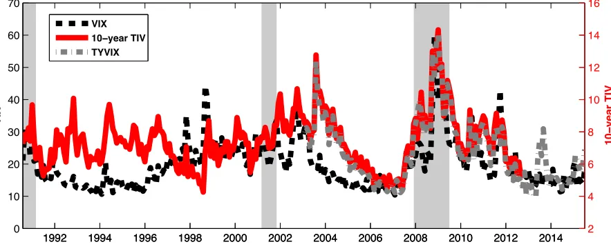
Vedolin (2016). Figure 1.1 provides a plot of the CBOE VIX, the CBOE TYVIX, and the 10-year TIV; following the custom in practice, they are the square root of the annualized

variances expressed in percent. The 10-year TIV is virtually identical to the TYVIX, and

they are largely correlated with the VIX. The bond VIXs are driven by the variance factor

in the discount rates (or the pricing kernel), while the VIX reflect the variance factor in

both the discount rates and cash flow dynamics. The figure shows that the impact of the

variance factor in the cash flow dynamics became less important from late 90s.

5_{See, e.g., Carr and Wu (2009), Drechsler and Yaron (2011), Bollerslev, Tauchen, and Zhou (2009), Ang,}

(16)

VIX

1992 1994 1996 1998 2000 2002 2004 2006 2008 2010 2012 2014 0

10 20 30 40 50 60 70

10

−

year TIV

1992 1994 1996 1998 2000 2002 2004 2006 2008 2010 2012 2014 2

4 6 8 10 12 14 16

VIX 10−year TIV TYVIX

Figure 1.1. TIV,TYVIX and VIX

This figure plots the CBOE VIX, the CBOE TYVIX and the 10-year TIV from Choi, Mueller, and Vedolin (2016). Volatilities are the square root from variances as constructed using option prices via equation (1.3). Numbers are annualized and expressed in percent. Gray bars indicate NBER recessions. The data is monthly and runs from July 1990 to June 2015; The 10-year TIV data ends in August 2012, and the TYVIX data starts from January 2003.

To summarize, Proposition 1 gives the implication of the model-free measure of im-plied volatility in the Treasury market, the bond VIX, once it is combined with additional

structures embedded in many economic models. Once the information in bond VIX is

in-corporated with an economic model in which the short rate is linear in Q aﬃne diﬀusion state variables, the bond VIXs can completely identify the volatility factors. This result

also implies that some economic fundamentals in macro-finance asset pricing models can be

identified via the bond VIX2_{s if the fundamentals determine the conditional variances of}

bond yields.

1.3 Predictability

The assumptions for Proposition 1 are that (i) the drift of a pricing kernel is affine in the state variable and (ii) the state variable follows affine diffusion under Q. Three classes of well-known consumption-based asset pricing models incorporate this feature. They are

the long-run risk framework of Bansal and Yaron (2004), the rare disasters framework of

(17)

Importantly, in all of these models, the source of time variation in risk premia is entirely

spanned by volatilities in yields only (see Le and Singleton (2013) for detailed explanations).

Once this salient feature of those models is incorporated with Proposition 1, it means that the bond VIX2_{s should predict future excess returns and they are the sole source of time}

variation in risk premia.

Specifically, the assumptions in Proposition1are canonical in most long-run risks models without jumps (or rare disasters) - see e.g. Bansal and Yaron (2004), Bollerslev, Tauchen,

and Zhou (2009), Bansal and Shaliastovich (2013), Zhou and Zhu (2015). For example,

in Bansal and Shaliastovich (2013), (i) the drift of the pricing kernel is a linear function

of the subset of aﬃne diﬀusion state variables - expected consumption growth, expected

inflation and their variance factors, and (ii) the P aﬃne state variable, in conjunction with their market price of risk, imply Q aﬃne state variable. The time-varying volatilities in expected consumption growth and expected inflation are the two economic fundamentals

that induce time variation in volatilities in yields. In this economy, Proposition1implies that the bond VIX2_{s should be the manifestation of uncertainty about the two macroeconomic}

fundamentals: expected consumption growth and expected inflation (see Appendix 2 for a formal derivation). Note that in long-run risk economies, the time-varying quantity of

macroeconomic risk is the only source of time variation in risk premia - the price of risk is

pinned down by Epstein-Zin preference. As a consequence, the bond VIX2_{s should capture}

the entire innovations in risk premia though the channel of time-varying quantity of risk.

The rare disaster framework with time-varying disaster probabilities is another example

that fits the assumptions of Proposition1- see e.g. Wachter (2013), and Tsai (2016). In this framework, the short rate is linearly dependant on time-varying risk of disasters (intensity

of a disaster more precisely). The intensity process follows aﬃne diﬀusion under both the

physical and the risk-neutral measures, and it also determines volatilities in yields. Then,

the bond VIX2_{s disclose the time-varying probability of a disaster because of Proposition} _1. Moreover, in this economy, time variation in risk premia solely stems from the time-varying

probability of a disaster. Hence, the bond VIX2_{s should have the ability to predict future}

(18)

The habit formation model in Le, Singleton, and Dai (2010), henceforth LSD, is another

class of asset pricing models in which the bond VIX2_{s should explain the entire time variation}

in risk premia. The model, based on Campbell and Cochrane (1999) and Wachter (2006),

uses the two assumptions in Proposition1to obtain aﬃne pricing. By doing so, they specify the market price of risk as a non-linear function of the states as in Duarte (2004) and, as a

result, the state variable follows a non-linear process under P. LSD shows that their model approximately nests Wachter’s model and closely resembles its prominent features. In this

type of aﬃneQ_{habit formation models with external habit level}_Ht_{, the consumption surplus} ratio st = log [(Ct₋Ht)/Ct] is the sole source of time-varying risk premia since the shocks

on consumption growth (that drives the quantity of risk in the economy) are assumed to be

homoscedastic. Furthermore, the volatilities in yields are driven by the non-negative process

ϕt = smax −st where smax is the upper bound of st.6 Hence, the bond VIX2 is linear in

ϕt, the inverse consumption surplus ratio, and contains the full information on risk premia

through the reflection of the time-varying price of risk.

Motivated by the implication of Proposition 1 for the three classes of asset pricing models, I examine whether the bond VIX2_{s explain time variation in expected bond excess}

returns. To assess their predictive ability, I initially apply MA2 filters for the one-month

bond VIX2_{s (with 5yr, 10yr and 30yr bonds as underlying assets) constructed in Choi,}

Mueller, and Vedolin (2016) with the aim of removing transitory shocks potentially due

to measurement errors and institutional eﬀects (see, for example, Kim (2007)). Then, I

regress one-year holding period excess returns of bonds with diﬀerent maturities onto the

space of the three (filtered) one-month bond VIX2_{, henceforth denoted as TIV}2_{s following}

Choi, Mueller, and Vedolin (2016). The projections indicate that, across all maturities,

the excess returns’ loadings on the TIV2_{s exhibit tent-shape pattern akin to the pattern}

in Cochrane and Piazzesi (2005). Hence, in the spirit of Cochrane and Piazzesi (2005), I

construct a single factor by projecting the average (across maturity) excess returns onto the

three TIV2_s:

rxt+12=γ0+γ1T IVt,5yr2 +γ2T IVt,10yr2 +γ3T IVt,30yr2 +et

6_{Note that}_s

(19)

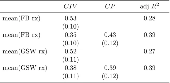
Table 1.1

Predictive Regressions

Panel A reports adjusted R2 from regressing twelve-month excess returns rx(n) of bonds with n years to maturity on CP factor, CIV, and both. Panel B presents estimated coeﬃcients from predictive regressions from the mean of excess returns in Panel A onto CP factor or (and) CIV. Standard errors are in parentheses and adjusted according to Newey and West (1987). Data is monthly and runs from October 1990 to December 2007.

Panel A: Predictive Regressions and Adjusted R2s

Excess returns from Fama-Bliss data Excess returns from GSW data

CP CIV CIV&CP CP CIV CIV&CP

rx(2) 0.20 0.27 0.36 rx(2) 0.15 0.26 0.31 rx(3) 0.22 0.28 0.38 rx(4) 0.21 0.28 0.36 rx(4) 0.24 0.28 0.40 rx(6) 0.25 0.27 0.38 rx(5) 0.22 0.28 0.38 rx(8) 0.27 0.26 0.39 rx(10) 0.28 0.23 0.38

Panel B: Predictive Regression Coeﬃcients

CIV CP adj R2

mean(FB rx) 0.53 0.28 (0.10)

mean(FB rx) 0.35 0.43 0.39 (0.10) (0.12)

mean(GSW rx) 0.52 0.27 (0.11)

mean(GSW rx) 0.38 0.39 0.39 (0.11) (0.12)

The time-series of the fitted values (henceforth, CIV) is the return-forecasting factor, and

is utilized to predict realized excess returns on each bond with maturity of n.

rx(n)_t+12=b(n)₀ +b(n)₁ *γˆ0+ ˆγ1T IVt,5yr2 + ˆγ2T IVt,10yr2 + ˆγ3T IVt,30yr2 +

+e(n)_t

For comparison purposes, the Cochrane-Piazzesi return-forecasting factor (henceforth, CP)

is constructed by regressing mean excess returns onto thespreads of five Fama-Bliss forward

rates with maturities of 1 through 5 years as in Cochrane and Piazzesi (2008). Excess returns

from the G¨urkaynak, Sack, and Wright (GSW) data set (with maturities of one through 10

years) are also utilized to assess excess returns on long-term bonds since the longest

(20)

Corr(CIV,CP) = 0.34 AutoCorr(CP) = 0.82 AutoCorr(CIV) = 0.82

1992 1994 1996 1998 2000 2002 2004 2006

-2 -1 0 1 2 3

mean(rx,GSW) CP

CIV

Figure 1.2. Excess Returns, CP and CIV

This figure plots the Cochrane-Piazzesi factor (CP),CIV, and the average of twelve-month excess returns on bonds with maturities of 1 through 10 years. Gray bars indicate NBER recessions, and blue bars represent financial crisis periods. The data is monthly and runs from October 1990 to December 2007.

Table 1.1 present adjusted R2_{s and coe}_ﬃ_{cients from predictive regressions of} twelve-month bond excess returns on CP, CIV, and both CP and CIV jointly. Panel B shows

that, for both sets (FB and GSW) of excess returns, each estimated coeﬃcient on CIV is

statistically significant during the sample period, and the variation in CIV explains more

than 20% of the variation in realized mean excess returns. Once CIV and CP are jointly

utilized, R2_{s increase more than 10 percentage points in addition to the statistical}

signifi-cance of both coeﬃcients. Panel A reports adjusted R2 _{from regressing each excess return}

on the predictors, and it reveals that the predictability of the CIV stems mainly from excess

returns of bonds with short-term maturities while the predictability of the CP comes from

relatively long-term maturities. As a result, the adjusted R2_{s are improved significantly}

once CIV and CP are utilized jointly to predict excess returns. Their joint significance can

(21)

CIV and CP exhibit heterogeneous movements and can assist each other to explain the time

variation in the excess returns.

1.4 Variance Risk and the Shape of the Yield Curve

How does volatility risk aﬀect the shape of the yield curve? Do yields strongly/weakly load

on volatility risk? Can we extract a reliable measure of interest rate volatility from the

cross-section of bonds? The first step to addressing these questions is to identify volatility

risk in a framework where volatility has a systematic impact on the yields across diﬀerent

maturities.

The class of aﬃne dynamic term structure models (henceforth, ADTSM) is a typical

ex-ample of such a framework, and has also served as the workhorse in the literature to assess

the impact of volatility risk on the cross-section of bond yields; ADTSMs are fully

character-ized by (i) the two assumptions in Proposition1, (ii) the specification of the market price of risk, and (iii) a set of parametric restrictions needed to identify the model. It is well

estab-lished that the aﬃne models successfully capture the cross-sectional properties of yields; see

for example Dai and Singleton (2000). However, the ADTSMs’ ability to capture variation

in the volatility of interest rates is questionable and controversial, especially once

volatility-sensitive derivatives are not incorporated into the estimation procedure of the model. For

instance, using U.S. swap data only, Collin-Dufresne, Goldstein, and Jones (2009) show that

the model implied volatilities from aﬃne models seem unrelated to their non-parametric or

semi-parametric counterparts (i.e. realized volatility estimates and GARCH estimates).

Because ADTSMs are built up on the two assumptions in Proposition1, the bond VIX2_s directly represent variance risk in the model. In other words, the variance risk in ADTSM is

readily identifiable via the bond VIX2_{s as a consequence of Proposition}_{1. This identification} strategy is beneficial in several ways. First, it is based directly on option prices that tend to

be more sensitive to the changes in volatility than nominal bond prices. This is in line with

previous studies pointing out that the introduction of volatility-sensitive instruments into the

estimation procedure can significantly mitigate the diﬃculty in identifying volatility risk of

(22)

(2011), Jagannathan, Kaplin, and Sun (2003), and Joslin (2014). In addition, the approach

doesn’t require us to estimate a specific model, and allows variance risk to be measured in

real time. Furthermore, since the variance measure is constructed in a model-free manner,

the approach can be easily incorporated into the class of Gaussian quadratic term structure

models, as in Ahn, Dittmar, and Gallant (2002). In this case, _Vt is a quadratic function of

the Gaussian state factors in the model 7 _{(See Appendix}₃ _{for a detailed explanation).}

Before estimating a fully-fledged model to analyze the impact of variance risk on the

cross-section of yields, I conduct two simple regression-based tests on the relationship

be-tween variance risk and the cross-section of yield. First, I examine the marginal impact

of the variance risk on the shape of the yield curve beyond the traditional term structure

factors: level, slope and curvature of the yield curve. The results suggest that variance risk

is largely unrelated to the shape of the yield curve and that at least three non-volatility

factors are required to adequately explain the cross-section of yields. The second test

investi-gates whether variance risk can be identified from the cross-section of yields: the unspanned

stochastic volatility (USV) eﬀect in Collin-Dufresne and Goldstein (2002). The USV eﬀect

can be or cannot be rejected, depending on the number of variance factors. The

empiri-cal evidence will be utilized as guidance for designing highly parameterized term structure

models in later sections.

1.4.1 The Shape of the Yield Curve and _Vt

Provided that (i) the state follows affine diffusion and (ii) the short rate is an affine function

of the state, the yield on a zero-coupon bond of maturity n is aﬃne in the state variableZt:

yn,t =An*ΘQ++Bn*ΘQ+Zt (1.5)

where An and Bn are obtained from standard recursions as in Duﬃe and Kan (1996). The

linear relationship between yields and factors in equation (1.5) implies that yields can be

treated as state variables; given a set of maturities equal in number to the number of latent

factors, one can rotate the underlying factor into the yields (see for example Pearson and Sun

7_{For Gaussian quadratic term structure models, the short rate equation is a quadratic function of}

(23)

(1994), Chen and Scott (1993) and Duﬃe and Kan (1996) among many others). One can

further rotate the risk factors into portfolios of yields, especially the principal component of

yields, _Pt, as in Joslin, Singleton, and Zhu (2011) for example. As will be shown thoroughly

in Section 1.5, Proposition 1 enables us to rotate the latent risk factors into portfolio of yields _Pt and portfolio of options Vt

y_to=_A+_BZZt=A+BPPt+BVVt+et, et∼N*0,σe2I +

(1.6)

where yto denotes a vector of stacked observed yields and et represents measurement error

assumed to be an independent and homoscedastic Gaussian random variable (as commonly

assumed in the literature). Because all the variables in equation (1.5) can be observable,

the yields’ loading on the factors_A,_BP and BV can be estimated by linear regressions. The

estimated model, then, can be treated as a standard linear factor model nesting the

no-arbitrage affine models since _A, _BP and BV are non-linear functions of ΘQ under the affine bond pricing models: see for example, Duffee (2011a), Hamilton and Wu (2012), Joslin and

Le (2014) and Joslin, Le, and Singleton (2013).

The marginal impact of the variance risk beyond traditional yield factors like level,

slope and curvature factors can be examined by comparing the likelihood of (1.6) with the

following restricted version of it:

yo_t =_A∗+_B_P∗_Pt+e∗t, e∗t ∼N *

0,σ_e2∗I

+

(1.7)

Table 1.2 reports the test statistics of the likelihood ratio test for the hypothesis of the zero coeﬃcients on the additional variable in the unrestricted version. The first column

presents the right hand side variables in the restricted models where PC1-PC3 denotes the

first, second and third principal components of yields on U.S. Treasury nominal zero-coupon

bonds with maturities of six months and 1 through 10 years8_{. The remaining columns present}

an additional variable in each version of the unrestricted model and its corresponding LR

statistics. VPC1 and VPC2 denotes the first and second principal components of the MA2

filtered 5, 10 and 30-year TIV2_{s as in Section} _{1.3. Each of VPC1 and VPC2 capture}

8_{The yields with maturities of two to ten years are from G¨}_{urkaynak, Sack, and Wright (2007). The}

(24)

Table 1.2

Marginal Impact of Variance Risks onto the Shape of the Yield Curve

This table reports the test statistics of the likelihood ratio test. The first column presents the right hand side variables in the restricted models: equation (1.7). The remaining columns present an additional variable in each version of the unrestricted model and its corresponding LR statistics. The last column shows the 5% critical value of the test statistics, which followsχ2_{(11) distribution.} Data is monthly and runs from October 1990 to December 2007.

Restricted Model Additional Variable in Unrestricted model VPC1 VPC2 PC3 PC4 C.V.(5%)

PC1, PC2 4.2 14.2 5882.9 19.7 PC1, PC2, PC3 45.0 18.6 3678.7 19.7

respectively 94% and 5.6% of the variation in the three TIV2_{s. The last column shows the}

5% critical value of the test statistics which followsχ2_{(11) distribution. The table indicates}

that for each version of the restricted model, its likelihood ratio is greatest when a yield

factor (PC3 or PC4) is the additional variable in the unrestricted model. In other words,

adding a PC factor to the restricted models is the best extension for the purpose of a better

cross-sectional fit. Moreover, for the unrestricted models with the variance factors as the

additional variables, the null can be rejected or not, but the magnitude of test statistics is

not very large, regardless of their statistical significance. Similar results are obtained once

two or three representative yields, instead of the yield PCs, are utilized as the right hand

side variables of the restricted models (the results are omitted in the paper for the sake of

brevity). In sum, the exercise indicates that the marginal benefit of adding variance factors

is fairly limited and it is hard to identify variance risk from the cross-section of yields.

The exercise also implies that it is empirically diﬃcult to extend the estimation approach

of Hamilton and Wu (2012) into aﬃne bond pricing models with stochastic volatilities.

They propose a minimum-chi-square estimation procedure of Gaussian ADTSM in which

the risk-neutral parameters of the model are inferred by minimizing the diﬀerences between

the ordinary least square (OLS) estimates of the cross-sectional equation (1.7) and the

corresponding yields’ loadings from Gaussian ADTSM. In theory, their approach can be

applied to equation (1.6) for the estimation of ADTSM with stochastic volatilities. However,

(25)

empirical implementation. The OLS estimates of _BV in equation (1.6) are not informative

enough to precisely pin down the risk-neutral parameters related to the volatility factors.

1.4.2 Unspanned Stochastic Volatility Eﬀect

The diﬃculty of identifying volatility risk under ADTSM stems from the multiple roles of

volatility risk in the class of aﬃne models. The volatility risk aﬀects (i) the second moments

of yields, (ii) the expectation of future interest rates under both physical and risk-neutral

measures, and (iii) the so-called convexity eﬀect introduced by the non-linear relationship

between bond prices and the latent factors. The various roles of volatility enables us to infer

it through multiple channels, but this feature causes tension rather than a complimentary

eﬀect in identifying it (see Joslin and Le (2014) for a detailed explanation).

One potential resolution for the issue is to impose a set of model-based restrictions to

remove the dependence of the cross-section of yields on volatility, a set of restrictions coined

as an “unspanned stochastic volatility” (USV) restriction by Collin-Dufresne and Goldstein

(2002). More broadly, the USV eﬀects mean that the yields curve itself fails to span the

volatilities in the changes in yields. In their seminar paper, Collin-Dufresne and Goldstein

(2002) define the USV eﬀect as the existence of a set of parameters _{φ1, ...,φN}that are not

all zero such that

N %

i=1

φiBn,i= 0 _∀n >0 (1.8)

where N is the number of pricing factors and Bn,i the i-th element of Bn in equation (1.5).

The authors further show that, under the existence of such a set of parameters with N _≥3,

one can find a rotation such that the variance factor Vt has no eﬀect on the price of bonds.

As a consequence, the variance factor cannot be extracted from the cross-section of observed

yields (see Collin-Dufresne and Goldstein (2002), and Joslin (2015) for further details).

The following studies, however, have accumulated conflicting evidence on the USV eﬀect.

Decoupling the dual role of volatility through the USV restrictions helps the model to

produce more realistic model-implied volatility, even though the model’s cross-sectional fit

is slightly impeded (see for example Creal and Wu (2015) and Collin-Dufresne, Goldstein,

(26)

of intraday volatility in yields is largely unexplained by term structure factors, which is in

line with the USV eﬀect. On the other hand, the USV eﬀect is rejected once the

model-specific restrictions are directly tested by the likelihood-ratio or the Wald test (Bibkov and

Chernov (2009), Joslin (2015)). Utilizing the observable volatility proxy, I devise a new test

for the USV eﬀects, which can shed new light on the debate.

The condition for the USV eﬀect in equation (1.8) can be translated into the statement

that the matrix _BZ ≡ [BP,BV] in equation (1.6) is not full rank, regardless the maturities

of the yields on the left hand side of the equation (see Appendix 5for a formal derivation). As a result, a statistical test for the rank of the estimated matrix ˆ_BZ is a test of the USV

eﬀect. The null hypothesis is

H0 : rank (BZ)≤N −1 (1.9)

where N is the total number of factors. I use the Kleibergen-Paap rank test, among many

other rank tests. The test statistic follows χ2 _{distribution: for details, see Kleibergen and}

Paap (2006).

The approach has several benefits not shared by other tests for the USV eﬀect in the

literature. First, it is a formal statistical test - many of others in the literature are not formal

statistical tests as pointed out by Bibkov and Chernov (2009). Second, while Bibkov and

Chernov (2009) and Joslin (2015) conduct formal tests for the set of restrictions generating

the USV eﬀect, the USV restrictions are not unique as pointed out by Joslin (2015). For

example, two diﬀerent sets of restriction on the A1(4) specification can induce the USV

eﬀect while the two models fit volatilities in significantly diﬀerent manners; see for example

Creal and Wu (2015). The rank test that I posit here is free from this issue. Finally, the

test can be implemented even in the presence of hidden factors as in Duﬀee (2011b) or

Joslin, Priebsch, and Singleton (2014) - a detailed explanation of the hidden factors can

also be found in Section1.6. The test only exploits the cross-sectional relationship between the yields and variance factors, so the test results should be identical even after taking into

account hidden factors.

Table 1.3 reports the test statistics for specifications with one through two volatility factors in conjunction with two through three additional non-volatility factors. Following

(27)

Table 1.3

Tests for the USV eﬀect

This table reports the test statistics of Kleibergen and Paap (2006) for the rank of the matrix _BZ in equation (1.6). The null of the test is equation (1.9). Data is monthly and runs from October 1990 to December 2007.

Specification Stat. d.f. C.V.(5%) p-val

A1(3) 20.82 9 16.92 0.01

A1(4) 20.72 8 15.51 0.01

A2(4) 14.90 8 15.51 0.06

A2(5) 14.89 7 14.07 0.04

The data set is the same as the one in Section1.4.1, and the firstm PCs of the MA2 filtered TIV2_{s are used as the variance factors for} _Am₍_N_{) models. Specifications with up to two}

volatility factors are considered for the exercise because the first two PCs of TIV2_{s explain}

99% variation of the three TIV2_{s as pointed out in Section} _{1.4.1. The table shows that, for} all the specifications, the null (the presence of USV eﬀects) is rejected at the 10% significance

level. Hence, the conditions for the aﬃne models to generate USV eﬀect do not hold in the

data.

In sum, it is true that variance risks are hard to identify from the cross-section of yields

as shown in Section1.4.1, however, the knife-edge conditions for the USV eﬀect are rejected in the data. In other words, the variance risk is eﬀectively unspanned by yields not because

of the USV restrictions but because of its limited impact on the shape of the yield curve,

and it can be hardly identified without help of option prices.

1.5 A New Representation of ADTSM

In this section, I suggest a new representation of ADTSM in which all factors are

repre-sented as portfolios of bonds and options. The representation inherits the spirit of Joslin,

Singleton, and Zhu (2011), and the advantages of their representation. Since all the term

structure factors (including volatility) are observable, the estimation procedure becomes

greatly simplified and economic interpretation of the model is more straightforward

(28)

For econometric identification, I initially assume that the risk-neutral dynamics of the

latent factor in equation (1.1) is drift normalized as in Joslin (2015) or Creal and Wu (2015).

The yield on a zero-coupon bond of maturity n is aﬃne in the states Zt:

yn,t =An*ΘQ+₊_Bn*_ΘQ+_Zt

where An and Bn are obtained from standard recursions as in Duﬃe and Kan (1996). I let

(n1, n2, ..., nJ) be the set of maturities of the bonds used in estimation andytbe the (J _×1)

vector of corresponding yields. For any full-rank matrix W _∈ R(N−m)×J, W yt represents the associated (N ₋m)-dimensional set of portfolios of J (_≥N) yields. Following Joslin,

Singleton, and Zhu (2011), I let_Pt denote the first (N −m) principal components (PCs) of

J yields with W being the weighting matrix of the PCs:

Pt=W yt=AW *

ΘQ+₊_B W

* ΘQ+_Z

t =AW *

ΘQ+₊_B W,X

* ΘQ+_X

t+BW,V *

ΘQ+_V t

Invoking Proposition 1, then, we can define the N observable pricing factors _Zt such that

Zt≡(Pt′,Vt′) ′

=*(W yt)′,_V_t′+′ =U0+U1(X_t′, V_t′)′ (1.10)

where

U0 = ⎡ ⎣ AW

α ⎤

⎦, U1 = ⎡

⎣ BW,X BW,V 0m×(N−m) β

⎤ ⎦

with αand β defined in Proposition1. The dynamic of_Zt can be represented as a function of the observable factor_Ztafter applying the invariant rotation of Dai and Singleton (2002)

to the latent factor Zt. Provided that the mapping between _Zt and Zt is bijective (i.e.

one-to-one mapping), the model with observable _Zt is observationally equivalent to the

representation with the latentZt. The suﬃcient condition for the mapping to be bijective is

a full rank matrix β. Once the Gaussian factorXt is drift normalized, Joslin (2015) shows

that the matrix BW,X should be full rank. Hence, the first (N ₋m) columns of U1 are

linearly independent. With non-zero β, the last m columns of U1 are not spanned by the

first (N ₋m) columns of U1, which implies that a full rank matrix β guarantees U1 to be

(29)

The new representation of ADTSM with the observable factors _Zt in equation (1.10)

follows the idea of Joslin, Singleton, and Zhu (2011), henceforth JSZ, and can be considered

an extension of their work into general aﬃne models. JSZ suggests a new representation

of Gaussian ADTSM in which all the Gaussian pricing factors are observable as portfolios

of yields, i.e. _Pt in equation (1.10). Through their representation, the estimation of the

Gaussian term structure model is extremely simplified, and becomes more reliable in terms

of finding a global optimum in maximum likelihood estimation. In particular, simple

or-dinary least square estimation (OLS) can be utilized to estimate the P conditional mean parameters of the pricing factors which had been treated as one of the most challenging

parts in estimating term structure models due to the high degree of persistence in yields.

In my representation, all pricing factors (including the variance risk), are observable. As

a consequence, one can make use of generalized least square estimation (GLS) to pin down

the drift of the pricing factor under P. Since variance is directly observational up to its linear transformation via _Vt, it is also easy to estimate the parameters governing the

time-series dynamics of _Vt. In addition, when volatility risk is identified from the cross-section

of yields, one should solve a numerically unstable equation AX =bwhere A is often nearly

singular, with the possibility that the solution leads to negative values for volatility: see

for example Piazzesi (2010) and Joslin (2014). Instead, the representation I posit here is

unaﬀected by this issue. In sum, the representation helps us find the global optimum of

maximum likelihood estimation by simplifying the two hardest parts of the ADT SM with

stochastic volatility estimation, namely, the identification of volatility, as well as the drift

of the state under P.

The parameterization scheme using portfolios of yields as pricing factors for Am(N)

model is also explored in Joslin and Le (2014), where the variance factor in Am(N) is

ap-proximated by portfolios of yields. The model I posit here utilize portfolios of options rather

than portfolios of yields, and the variance factor is known before the model estimation while

their variance factors can only be identified after the model estimation. In addition, the

approach here is robust even in the presence of unspanned stochastic volatility factors as

(30)

(without options) results in undesirable properties in the factor dynamics under P - this issue is discussed further in Section 1.7.2.

1.6 Unspanned Macro Risk and the Likelihood Function

More recently, a large literature has been studying so-called hidden factors or unspanned

macro factors, see e.g., Duﬀee (2011b), Chernov and Mueller (2012) and Joslin, Priebsch,

and Singleton (2014), henceforth JPS. A factor is described as hidden if it plays an important

role in determining investors’ expectations for future yields, yet is not priced in the fixed

income market. Hence, the hidden factor cannot be recovered from the cross-section of any

fixed income assets. This section explains how to take into account the hidden factor inside

the model described in the previous section.

Since all priced factors are observable due to the representation in the previous section,

the same argument as in JPS can be applied in order to add hidden factors in the framework.

Once both hidden and non-hidden factors are projected onto the space of fixed income asset

returns as in JPS, we get the following factor dynamics under the physical measure P and the risk-neutral measure Q. First, the factors are composed of (i) the priced risks in the fixed income market _Zt = (Pt′,Vt)′ and (ii) a non-priced (hidden) factor Mt. In discrete

time setting, the dynamics of the non-variance factors, (_P′

t, Mt), can be represented as ⎡

⎣ Pt+1 Mt+1

⎤ ⎦=

⎡ ⎣ K0PP

KP 0M

⎤ ⎦+

⎡

⎣ KPPP KPPM KP

MP KM MP ⎤ ⎦ ⎡ ⎣ Pt

Mt ⎤ ⎦+

⎡ ⎣ KPVP

KP MV

⎤ ⎦_Vt+

⎡ ⎣ ΣPV

ΣMV ⎤ ⎦ϵP

V,t+1+ ⎡ ⎣ ϵP,t+1

ϵM,t+1 ⎤ ⎦ (1.11) with *

ϵ′_P_,t+1,ϵ′_M,t+1+′ _∼ N(0,Σt)

Σt = Σ0+Σ1(_Vt−α) (1.12)

ϵP

V,t+1 = Vt+1−Et(Vt+1)

The variance factor _Vt+1 follows a compound autoregressive gamma process

Vt+1|Vt∼CAR *

(31)

wherecP_{is a scale parameter,}_νP _{is a shape parameter, and}_ρP_{determines the autocorrelation} of _Vt. The lower bound of Vt is set α, contrary to the standard lower bound of zero for a

variance process. Indeed, the lower bound of the latent variance factor Vt should be set to

zero for econometric identification. Then, the linear relationship between the observable _Vt

and the latentVt,_Vt=α+βVtwithα *

ΘQ+_{defined in Proposition}_{1, implies that}

Vtshould be greater thanα. Furthermore,αshould be positive since bothα*ΘQ+_and_β*_ΘQ+_capture the convexity components of yields - see equation (A-8) and Appendix 4.2 for details. The non-zero lower bound of_Vtalso leadsΣtin equation (1.12) to beΣ0+Σ1(Vt−α) rather than

Σ0+Σ1_Vt. For a detailed explanation of compound autoregressive processes, see Gourieroux

and Jasiak (2006), Le, Singleton, and Dai (2010) and Creal and Wu (2015).

Under the pricing measure Q, the dynamics of_Zt are assumed to be

Pt+1 = K0QP +K Q

PPPt+KPVQ Vt+ΣPVϵQV,t+1+ϵP,t+1 (1.13)

Vt+1|Vt ∼ CAR *

ρQ, cQ,νQ,α+

Hence, the specification of the price of risks follows that in Cheridito, Filipovi´c, and Kimmel

(2007), and yields can be represented as a linear function of (_P′

t,Vt)′ where yields’ loadings

on the pricing factors are determined by ΘQ _{(see Appendix} _4.1).

Furthermore, in order to maintain (i) the diﬀusion invariance property of the variance

process _Vt and (ii) non-exploding market price of risk in the continuous time limit (see

Ap-pendix B.4 in Joslin and Le (2014) for explanations), I impose the following two restrictions

on parameters for _Vt:

cP =cQ, νP =νQ

For the fitting of the cross-section, I assume that higher-order PCs, denoted by _Pe,t, are

observed with i.i.d. uncorrelated Gaussian measurement errors with a common variance:

Pe,to =Pe,t+et and et ∼N *

0, Iσ_e2+

In sum, the likelihood function of the observed data, _L, is

(32)

where f denotes the log conditional density. The first two terms capture the density of the

time-series dynamics, and the last term is the density of the cross-sectional fit on which the

unspanned macro factorsMt have no impact. Particularly, theP-feedback matrix of_Pt and Mt can be concentrated out by running GLS of the following system:

⎡

⎣ Pt+1 −ΣPVϵ P V,t+1

Mt+1₋ΣMVϵPV,t+1 ⎤ ⎦= ⎡ ⎣ K P 0P KP 0M ⎤ ⎦+ ⎡ ⎣ K P

PP KPPM KP

MP KM MP ⎤ ⎦

⎡ ⎣ Pt

Mt ⎤ ⎦+ ⎡ ⎣ K P PV KP MV ⎤ ⎦_Vt+

⎡ ⎣ ϵP,t+1

ϵM,t+1 ⎤ ⎦

The observable variance _Vt can be either spanned by yields or unspanned (i.e. of the

unspanned stochastic volatility type as in Section 1.4.2). However, this does not aﬀect the estimation procedure, since the volatility factor is identified not via yields but via options,

even before the estimation procedure. In contrast, without the observable volatility factor,

one should choose a specific set of restrictions on the Q parameters (among many possible set of restrictions), in order to estimate a model with unspanned stochastic volatilities.

Otherwise, the identification of the volatility factor is infeasible, because it has no eﬀect on

the price of bonds.

In the term structure literature, both the unspanned stochastic volatility and hidden

factors have been considered important components driving the time variation in risk premia,

although their mechanisms are totally diﬀerent. The eﬀect of hidden factors on changes in

risk premia exactly cancels out its eﬀect on expectations of future short rate while USV

implies a cancelation of the convexity bias. The USV factor can be identified from interest

rate derivatives while hidden factors cannot be identified from any financial instrument in the

market. To the best of my knowledge, my model is the first one capable of accommodating

both types of unspanned risks: the unspanned stochastic volatility factors as well as the

hidden factors.

1.7 Model Comparison

1.7.1 Model Specifications and Data

(33)

three term structure factors, level, slope and curvature. Under the representation in Section

1.5, this implies that at least three Gaussian factors are required to adequately explain the shape of the yield curve. Hence, I study a model with three yield factors and one stochastic

volatility, which I denote by A1(4) as in Section 1.4.2. Its corresponding specification with two unspanned macro risks, denoted as UMA2

1(6), is also investigated; UMARm(N) stands

for the family of ADTSMs in Section1.6, with (_P′

t, Mt′,Vt′) ′

of dimensionN,Mtof dimension

R, and_Vt of dimensionm. Following JPS, I use measures of economic activity and inflation

as the two unspanned macro risks. In particular, the three-month moving average of the

Chicago Fed’s National Activity Index (CFNAI), henceforth denoted as GRO, is used as

the measure of the growth in real economic activity as in JPS. However, I use

year-over-year growth in Consumer Price Index excluding food prices and energy prices (henceforth,

CP I) for the measure of inflation, contrary to JPS in which the measure of inflation is the

expected rate of inflation from Blue Chip Financial Forecasts (henceforth, INF).

Moreover, the same UMA2

1(6) specification but with a diﬀerent measure of economic

ac-tivity - the unemployment gap - is also studied. The unemployment gap (henceforthUGAP)

is the diﬀerence between the actual unemployment rate and the estimate of the natural rate

of unemployment from the Congressional Budget Oﬃce (CBO). Hence, it gauges thelevel of

economic activity rather than the growth of activity. Bauer and Rudebusch (2016),

hence-forth BR, argue that level indicators of activity such like UGAP are largely related to the

movement of the yield curves (i.e. weakly unspanned by yields) because these variables are

relevant for setting the short-term policy rates; the authors also point out that the

em-pirical monetary policy rules literature has identified level rather than growth variables as

those which are most important for determining monetary policy (e.g. Taylor (1993), Taylor

(1999), Orphanides (2003), Bean (2005) and Rudebusch (2006) among others). On the other

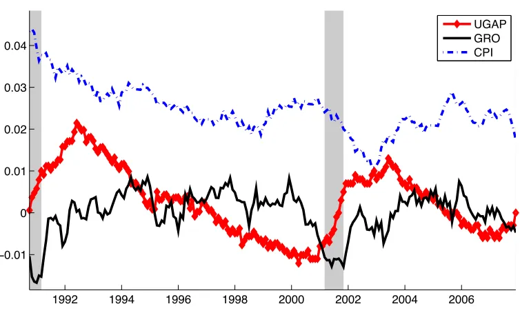
hand, measures of growth in economic activity such as GRO are largely uncorrelated with

the level of activity; see for exampleUGAP andGROin Figure1.3. Furthermore, BR show that growth variables accompany low R2_{s when (i) they are projected onto term structure}

factors or (ii) fed fund rates are regressed on them. Hence, they are strongly unspanned

by yields. The diﬀerent spanning properties of UGAP and GRO induce significantly

dif-ferent estimates of risk premia for the UMA2

(34)

1992 1994 1996 1998 2000 2002 2004 2006 −0.01

0 0.01 0.02 0.03 0.04

UGAP GRO CPI

Figure 1.3. UGAP, GRO and CPI

This figure plots the unemployment gap (U GAP), the three-month moving average of the Chicago Fed’s National Activity Index (GRO) and the year-over-year growth in Consumer Price Index, excluding food prices and energy prices (CP I). Gray bars indicate NBER recessions. The data is monthly and runs from October 1990 to December 2007.

the relevance of two diﬀerent estimates of risk premia and claim that UGAP is a better

measure of economic activity. I access four unspanned models UMA2

0(5) and UMA21(6)

and evaluate their relevance based on whether they can match the pattern for violation of

the expectations hypothesis.

The yield data set is the same as that in Section1.4, but I only use yields with maturities of six months, 1 through 3 years, 5, 7, 9 and 10 years. As a measure of observable volatility,

I make use of the 30-year TIV.

1.7.2 The Campbell and Shiller Regression

The most well-known stylized fact in the fixed income market is the failure of the

expecta-tions hypothesis (see, for example, Fama and Bliss (1987) or Cambpell and Shiller (1991)

among many others). As pointed out by Dai and Singleton (2002), this prominent