Monte Carlo Simulation and Improvement of Variance Reduction Techniques

2017 International Conference on Mathematics, Modelling and Simulation Technologies and Applications (MMSTA 2017) ISBN: 978-1-60595-530-8

Monte Carlo Simulation and Improvement of Variance

Reduction Techniques

Zi-xuan CAO

*

, Zhuo YANG, Kun LIU, Ze-wei ZHANG, Zi-ting LUO

and Zhi-gang ZHANG

University of Science and Technology Beijing, 30 Xueyuan Road, Haidian District, Beijing, China *Corresponding author

Keywords: Monte Carlo Simulation, Variance Reduction, Efficiency.

Abstract. Variance reduction technique is an important method to improve the efficiency of Monte Carlo simulation. In order to research the principle of reducing variance, we introduce Monte Carlo simulation firstly; then enumerate several commonly used methods of variance reduction and furtherly combine them to study whether it improves the simulation performance; lastly, we write programs to compare the reduction rates of different methods on the same problem. It turns out that variance reduction techniques have remarkable effect on increasing the calculation accuracy and reducing the calculation time of Monte Carlo simulation. And the combination of multiple variance reduction techniques is more effective in practical application.

Introduction

The development of Monte Carlo method has undergone a long period of time. In 1977, French physicist Buffon put forward the method of calculating PI by needle experiment, which established a theoretical foundation for its emergence. In 1940s, in order to adapt to the development of atomic energy at that time, American mathematician Ulam and von Neumann found the theory of probability and statistics. This method was named by a famous gambling city Monte Carlo in Monaco. In recent years, people have made great improvement on Monte Carlo method. More and more effective ways are found to improve simulation accuracy, including variance reduction techniques.[1]

Different variance reduction techniques have their own scopes of application. For example, antithetic variable method is suitable for symmetrical distribution; while control variable method is applicative when the controlled variable and the estimated variable have strong correlation; the key to conditional expectation method is to find a known conditional expectation; and importance sampling method depends on the selection of the importance function, so that the complex distribution can be replaced by a common and easily sampling distribution.

In practice, however, there is a lack of horizontal comparison between different variance reduction techniques. And the combination of multiple methods is not deeply researched so far. Therefore, this paper studies the combination of multiple techniques based on four basic methods. It is hoped that the results can be used for reference in practical problems.

The Basic Principle of Monte Carlo Simulation

The main idea of Monte Carlo simulation is to calculate the true value approximately by simulating a random variable. The basic methods are as following. Firstly, construct a probability model, which satisfies that the solution of this model is also the solution of the demand problem. Then calculate the statistical characteristics of the required parameters by observing or sampling the model. Finally, use the arithmetic mean of these values as the approximate value of the demand problem.

Suppose A is a required value of the solution, we can assume that A is the expected value of

 

is an approximate solution of A, which is the expectation of a series of independent random variables obtained by repeated sampling of X .

 

   

E h X h x f x dx

 _ _



(1) According to the strong law of large numbers, we can get





lim



1

P  A

   (2)

The mean of samples  is called the Monte Carlo estimator of A, which is an unbiased estimator of A. Let 2 be the variance of h X

 

, and m be the amounts of sample points, then the variance of estimator  is



 

1

 

i 2

i

Var Var h X

m m

   _ _





 (3)

According to the central limit theorem, the estimation error of the Monte Carlo method satisfies

 Z 2

m 



     (4)

In which

2

Z_ is the ₂ site in the standardized normal distribution.[2] The above equation shows

that the simulation error is inversely proportional to the square of the number of experiments m, and is proportional to the standard deviation  . In order to improve the accuracy and reliability of the estimation, we can increase the number of experiments or reduce the variance of simulated variable. But in practical problems, it is hard to increase the amounts of sample points and will take a long time. So when simulating a small probability events, how to control the variance of estimated value or to improve sampling method is the focus of our research now.

Several Common Methods of Variance Reduction

Variance reduction means that the original Monte Carlo simulation method can be improved by using a smaller unbiased estimator or a new sampling method, so as to achieve the purpose of improving the accuracy of calculation. At present, the most commonly used variance reduction techniques include antithetic random variable method, control variables method, conditional expectation method, and importance sampling method and so on. The principle of variance reduction will be theoretically derived in detail.

Antithetic Random Variable Method

As the name suggests, the method of antithetic random variable utilizes symmetrical characteristic of symmetry distribution, such as normal distribution. It selects a pair of antithetic variables



X,X



to carry out simulation. In this way, a variable X obeying the same distribution can be generated while generating a variable X that obeys a certain distribution. Thus, this method can save half of the time to call the generating function and improve the computing efficiency.[3]

If we suppose the parameter to be estimated is A, which is equal to E X

 

. X₁ and X₂ are identical distributed random variables of expectation A, satisfying that X₁ X₂, then we can get

 

 





1 2

1 2 1 2

1

2 ,

2 4

X X

Var_   _ _Var X Var X  Cov X X _

Because X₁ X₂,

 

1

 

2

Var X Var X ,Cov X X



₁, ₂



0 (6) So we can get

 

1

 

2

 

1

1 2

2 4 2

Var X Var X Var X X X

Var_   _  

  (7)

In the same way, it can be obtained that

2

1 1 1

1 1 1

2

n n n

i i i

i i i

Var X X Var X

n  n  n 

 _{ } _  

   







 



 (8)

That is to say, the method achieves the goal of reducing the variance.

However, due to the selection of antithetic variables requires strict negative correlation between two variables, the antithetic random variable method is only applicable to symmetric distribution, which is the biggest limitation of the method.

Control Variable Method

Control variable method improves the estimation of Monte Carlo integral by connecting estimators with the related Monte Carlo integral.

Supposing we use the simulated method to estimate A, which is equal to E X

 

. Here the random variable X is one of the output results of simulation, and Y is another output result. Now we consider another estimator of E X

 

, which is





cv Y

X  X c Y (9) Where _Y is the expected value of Y, c is an arbitrary constant. Obviously, X_cv is an unbiased estimator of A.Considering the variance of X_cv,













 

2

 

₂



_,



Y

Var Xc Y Var XcY Var X c Var Y  cCov X Y (10) Suppose that when _cc*_{, the value of}

 

cv

Var X can obtain the minimum. It can be calculated that





 

* Cov X Y,

c

Var Y

  (11)

Then the minimum variance of estimator is







Y



 

2



 

,



Cov X Y Var X c Y Var X

Var Y



    (12)

When X and Y are positively correlated, c* is negative. If the simulation result value Y is greater than the known mean value _Y, X may also be greater than its mean value . Therefore, we can modify the value of X by reducing its value, which is to make the value c* negative. A similar discussion can be made, when X and Y is negatively correlated. It can be seen that the quantity Y has a control effect on the random variable X . So Y is called the controlled variable of simulated estimator X . When simulating multidimensional random variables, multiple controlled variables can also be introduced.









 





* 2 1 , Y

Var X c Y

Corr X Y Var X



 

  (13)

In which









 

 

,

, Cov X Y

Corr X Y

Var X Var Y

 (14)

is the correlation coefficient of X ,Y. Using the method of control variable can reduce the estimated variance by ₁₀₀ 2



_,



_%

Corr X Y . And the stronger the correlation between the controlled variable Y and the random variable X , the better the effect of the variance reduction.

In general, we do not know the values of Cov X Y



,



and Var Y

 

in advance, so they need to be estimated by simulation. For the n time output results X_i and Y, i1, 2, , n, we apply the two formulas 











1 1 , 1 n i i i

Cov X Y X X Y Y

n 

  





(15)



 





2

1 1 1 n i i

Var Y Y Y

n 

 





(16)

Then the approximate values of *

c can be obtained, which is













1 * 2 1 n i i i n i i

X X Y Y c Y Y       





(17) In this way, the variance of the controlled variable







*



1

 

2



 

,



Y

Cov X Y

Var X c Y Var X

n Var Y

  

   _  _

  (18)

can be estimated by the estimated values of Cov X Y



,



and Var X

 

, Var Y

 

.

Conditional Expectation Method

The principle of conditional expectation method is to replace the original variable with the known condition expectation to carry on the simulation estimation.

Assuming that the parameter AE X

 

is to be estimated. X is a random variable, and Y is another random variable. If E X Y



|



is known, it can be used as a new estimator. Because



|





|



E E X Y_  _ E X Y  A (19)



|



E X Y is also an unbiased estimator of A. According to the formula of conditional variance

 

 

|





|





Var X E Var X_ Y_Var E X Y (20) We can know

 





|





Var X Var E X Y (21)

Importance Sampling Method

The importance sampling method estimates the expectation of the new variable by selecting a special density function. Its principle originates from the idea of variable substitution in mathematics, which is

 

   

 

 

   

1 1 1

0 0 0

f x f x

f x dx g x dx dG x

g x g x

 







(22) The selection of random variables at this time is no longer uniform, but distributes in the cumulative distribution function G x

 

.

In the importance sampling of the original weight, the new integrand is f x

 

multiplied by weight

 

1 g x . The g x

 

dG x

 

dx in the formula is called a bias distribution function. The expectation of the variable can be expressed as

 

   

f x

   

 

E h X h x f x dx g x dx g x

 _ _







(23)

Sampling independent and identically distributed variables X X₁, ₂, , X_m from g x

 

. Then the estimated value for  is

 1

   

i i

i

h X X

m





 (24)

Where  in the formula is the original weight, 

 

X_i  f X

   

_i g X_i . If the selection is appropriate, and makes the shape of the function curve in the integral domain is close to that of f , then the variance can become very small.[4]

As a result, we have the following requirements for the distribution function:

 

g x should be a probability density function; f x

   

g x should not be undulating in the

integral domain but be as constant as possible to ensure that the variance Var f g





is smaller than

 

Var f ; the cumulative distribution function G x

 

corresponding to the probability density

function g x

 

should be easily analytically obtained; and random variables which satisfy the cumulative distribution function G x

 

in the integral domain should be generated conveniently.

However, in the sampling process, the average value of all the new variables is taken as the final result, so there may be errors. In order to reduce the error, we use the average of the weight function instead of the original weight, which called the importance sampling method of the standard weight. The principle of the important sampling method of the standard weight is the same as that of the original weight, and the expectation can be expressed as

 

   

 

   

   

 

   

f x

h x g x dx h x f x dx _{g x}

E h X

f x f x dx

g x dx g x

 _ _











(25)

Sampling independent and identically distributed variables X X₁, ₂, , X_m from X X₁, ₂, , X_m. Then the estimated value for  is



   

*

i i

i

h X X

Where _* _{is the standard weight,} *

 

 

 

i i i

X X X

 



 . The important sampling of standard weight can also achieve the goal of variance reduction, and reduce the error to a certain degree.

The importance sampling method is undoubtedly one of the most basic and commonly used techniques in Monte Carlo computation. It has great potential both in reducing the computing time and increasing the stability of numerical results. But there are still some limitations: Firstly, to find a probability density function g x

 

, and obtain the corresponding cumulative distribution function

 

G x analytically is not an easy work; secondly, when the selected g x

 

at a certain point is zero or very quickly tends to zero, this is very dangerous in the numerical calculation of this point. The variance Var f g





is also likely to be large. This problem can not be detected by the usual method of estimating variance from the sample point, which can make the calculation result unstable.

Simulated Calculation Based on Variance Reduction Techniques

The past decades have witnessed the extensive application of Monte Carlo simulation in the field of Finance and Engineering. As a result, variance reduction techniques have become more and more important in improving its accuracy and reducing computational tasks. In the following parts, there are two examples showing the effect of variance reduction techniques, which include estimating the approximation of PI and the approximation of a certain integral.

The Application of the Variance Reduction Techniques on Estimating the Approximation of PI

Monte Carlo simulation originated from Buffon needle experiments for the approximation of PI. Assumed that there is a square in the first quadrant with the side length equal to 1. And in this square, there is a quarter of unit circle whose center is the original point and radius equals to the side length of the square. Now there are two random variables which are independent to each other and obey the uniform distribution in the interval

 

0,1 . Then the random variables



X Y,



correspond to a random point in the square. From the classical probability formula, we can see that the probability of random points falling within 1/4 circle is



2 2 ₁



1 4

4 theareaof circle P X Y

theareaofthesquare



    (27)

If there are a large number of random points in the square, we can calculate the frequency of the points falls inside the 1/4 circle as the approximate probability, then we can get the approximate value of PI.[5]

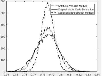
[image:6.612.218.396.600.734.2]

In order to make comparison, we calculate the value of PI by using original Monte Carlo simulation, antithetic variable method and conditional expectation method respectively. In the 10000 times simulation, we throw 1000 random points each time, and count the frequency of each probability interval. The scatter plot is made as follows.

Table 1. The reduction rates of three ways (calculate PI).

The transverse axis indicates the probability of falling within the 1/4 circle, and the longitudinal axis represents the frequency within each small probability interval. From the graph we can see obviously that the probability distribution of antithetic variable method is slightly concentrated compared with the original Monte Carlo simulation. Its effect of variance reduction is not obvious. But after the application of conditional expectation method, the distribution of data is much concentrated. Thus, the conditional expectation method can decrease the variance of estimators significantly. After further calculation we find the variance is reduced about 70% using this method.

The Application of the Variance Reduction Techniques on Estimating Integral

Next, we respectively use the original Monte Carlo simulation method and different variance reduction techniques to estimate the approximate value of integral

 

1 1

2

0 01

x

e

h x dx dx

x

  







(28) Because the integrand function h x

 

is monotonic in the interval

 

0,1 , the antithetic variable method can be used. Besides, the controlled variable _{t x}

 

_ex _{is close to the integrand, so the}

control variable method can also be used to reduce the variance. When using the importance sampling

method, we choose the importance function

 

₁ 1

x

e g x

e

 



 , which satisfies the condition

 

1

0g x dx1

[image:7.612.99.512.484.597.2]



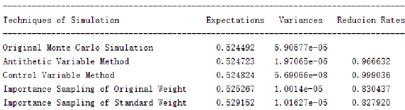
. The computing results are as follows:

Table 2. The reduction rates of five ways (calculate integral).

Observing the results, we find in the calculation, antithetic variable method can reduce 96% of the variance effectively; control variable method has the best effect, in which the variance can be reduced more than 99%; however, the reduction rate of importance sampling method of original weight and standard weight are only about 83%, and the difference between these two methods is not obvious. That is because the integral calculation process is relatively regular. In the physical problem, these two importance sampling methods will generally have different variance reduction rates.

The Improvement of Variance Reduction Techniques

simulation of the estimated value will be more accurate and the efficiency will be further improved.

The Improvement of Conditional Expectation Method

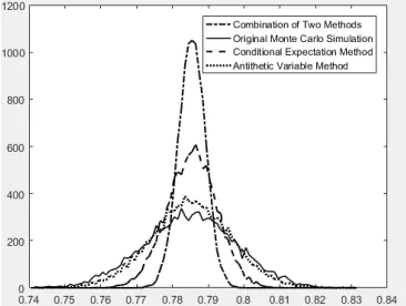
[image:8.612.214.397.152.290.2]

Above all, we introduce antithetic variables in the conditional expectation method, and calculate the approximate value of PI with the same method. Then we compare the variance reduction rates before and after the improvement. The results are as follows:

[image:8.612.107.506.332.431.2]

Figure 2. The frequency distribution graph of improved four ways (calculate PI).

Table 3. The reduction rates of improved four ways (calculate PI).

Based on the results, we can find that when the conditional expectation method is combined with antithetic variables, the reduction rate of variance can reach 91%, which is significantly improved compared with the single conditional expectation method. From the frequency distribution graph, we can also conclude that the combination of the two methods has a good effect on reducing the variance.

The Improvement of Importance Sampling Method

Combine importance sampling method with antithetic variables, and calculate the approximate value of integral in 3.2. Then we compare the variance reduction rates before and after the improvement. The results are as follows:

Table 4. The reduction rates of improved four ways (calculate integral).

[image:8.612.94.515.581.680.2]

Conclusion

In this paper, the effects of multiple variance reduction techniques and their combination on the practical problems are compared and analyzed. The results show that using control variable method to improve integral calculation can achieve a high variance reduction rate. And its effect is much better than any other methods in terms of computation accuracy and convergence speed. On the other hand, the combination of conditional expectation method and importance sampling method with antithetic variable can also improve the effect of the variance reduction on the original basis. Therefore, the combination of variance reduction techniques is of great practical significance for reducing the simulation calculation of Monte Carlo and improving the computation accuracy of Monte Carlo simulation.

References

[1] Sheldon M. Ross, Simulation, 4th ed., Elsevier Pte Ltd, Singapore, 2007, pp. 113-175. [2] Li Jihua, Monte Carlo Method, Building Structure. 11(1994) 3-8.

[2] Wei Yanhua, Wang Bingcan, Reduction of Monte Carlo Variance by Controlling Variables, Statistics and Decision. 470(2017) 71-73.

[3] Zhi Dongxiao, Empirical Comparison Among Ways of Variance Reduction, Statistical Thinktank. 109(2008) 20-23.

[4] Wang Lixue, Sun Jubo, Xu Pingfeng, Monte Carlo Method and Comparison Analysis of Variance Reduction Techniques, Journal of Changchun University of Technology. 36(2015) 485-489.