© 2016, IRJET | Impact Factor value: 4.45 | ISO 9001:2008 Certified Journal
| Page 1111
PERFORMANCE ANALYSIS OF MEDICAL IMAGE USING GRAY LEVEL
CO-OCCURRENCE
Muneer Ahamad
Research Scholar in Electronics and Communication Department, Mewar University, Rajasthan, India
---***---Abstract-
When researchers square measure finding out the detection of brain tumours and ultrasound abnormalities. Now aday there is a trend to analyse the brain tissue with the help of CT scan images. CT scan images are captured by CT scan machine, but these images are not correct for analysis to declare kind of disease, so prior to generate the report it is necessary to apply image processing. Image processing includes image resizing, filtering, accessing region of interest, enhancement, feature extraction, segmentation and reconstruction. In this paper feature extraction has been performed using grey level co-occurrence matrix method. Feature extraction is performed on ultrasonic image and CT scan of brain images. The extraction of the textural options of the metameric region of interest is finished by victimization grey level co-occurrence matrices (GLCM) technique that is extracted from four different orientations; horizontal orientation, left diagonal orientation, vertical and right diagonal lobe (0)°, (45)°, (90)°, and (135)° and two picture element distance for three completely different windows sized blocks. One is 8x8 second is 16x16 and third is 32x32.In this paper the results are analysed for the grey level co-occurrence matrices at 0°, 45°, 90° and 135° with 8x8 size of window produces informative options to classify between abnormal and non-masses. Our technique was able to accomplish correctness of ninety three percent and sensitivity of 12%
Keywords:Medical Images, CT scan images, Masses, GLCM
1. INTRODUCTION
Images play a vital role in today’s age of compact data. The sector of image process has exhibited monumental progress over past few decades. Generally, the pictures dealt in virtual environments or diversion applications possess sound reproduction leading to giant storage needs. Pictures might bear distortions throughout preliminary acquisition method, compression, restoration, communication or final show. Therefore image quality mensuration plays a major role in many image-processing applications. Image quality, for scientific and medical functions, will be outlined in terms of well desired data that will be extracted from the image. A picture is alleged to own acceptable quality if it shows satisfactory utility, which suggests discriminability of image content and satisfactory naturalness, which suggests identifying characteristics of image content. Digital storage of pictures has created a vital place in imaging. Image quality metrics square necessary performance variables for digital imaging systems and square measure wont to measure the visual quality of compressed pictures. The three major styles of quality measurements square measure [14].
Braintumour based diseases are the top causes of death for human being throughout the world. The average human has one probability in twelve of generating carcinoma throughout his life. Abnormalitiesin brain decrease the thinking power because of carcinoma is being recognized by the first detection of carcinoma mistreatment the screening diagnostic technique [1] [2]. However it is currently a tough decision to acknowledge the uncertain irregularities in brain CT scan images instead of the rise in technology. It is observed that the first diagnostic technique informs comparatively low distinction pictures, particularly within the case of serious brain condition and second; signs of irregular tissue might stay perfectly refined. For instance, speculated plenty which will indicate a malignant tissue at intervals the brain square measure typically tough to observe, particularly at the first stage of development [3]. The recent use of the second order statistics and machine learning (ML) classifiers has established a brand new analysis direction to observe plenty in digital X-ray photograph. The second order statistics of brain tissue on CT scan images remains a difficulty of major importance in mass characterization. Compared to alternative mammographic diagnostic approaches, the mammographic has not been studied full attributable to the inherent problem and opaqueness [4]. During this paper, GLCM options of X-ray photograph pictures square measure analysed. This work is organized as follows. In Section two we have a tendency to gift connected works for detection of plenty in X-ray photograph pictures. In Section three GLCM and options square measure explained. In Section four, the informative analysis is completed and therefore the results square measure shown. The last Section five has the conclusion and proposals. In applied math texture analysis, texture options square measure computed from the organization of ascertained mixtures of intensities at such positions relative to every alternative within the image.
© 2016, IRJET | Impact Factor value: 4.45 | ISO 9001:2008 Certified Journal
| Page 1112
2. METHODOLOGY
Fig- 1: Method to Implement System
2.1 IMAGE PREPROCESSING Resizing Image
Image interpolation happens once you size or distort your image from one part grid to a special. Image resizing is very important once you've got to be compelled to extend or decrease the general form of pixels, whereas remapping can occur once you unit of measurement correcting for lens distortion or rotating an image. Zooming refers to increase the quantity of pixels, so as that when we zoom an image, we will see further detail.
Interpolation works by exploitation known info to estimate values at unknown points. Image interpolation works in a pair of directions, and tries to comprehend a best approximation of a pixel's intensity supported the values at encompassing pixels. Common interpolation algorithms are going to be sorted into a pair of categories: adjective and non-adaptive. Adjective ways change depending on what they are interpolating, whereas non-adaptive ways treat all pixels equally. Non-adaptive algorithms include: nearest neighbour, bilinear, bicubic, spline, sinc, lanczos et al. adjective algorithms embody many proprietary algorithms in approved code such as: Q image, photo zoom skilled and real Fractals.
Many compact digital cameras can perform every associate optical and a digital zoom. A camera performs associate optical zoom by moving the camera lens so as that it will increase the magnification of sunshine. However, a digital zoom degrades quality by just interpolating the image. The photograph with digital zoom contains constant form of pixels, the detail is clearly most however with optical zoom.
Image improvement is actually rising the interpretability or perception of information in footage for human viewers and providing higher input for different automated image method techniques. The principal objective of image improvement is to vary attributes of an image to make lots of applicable for given task and a particular observer. Throughout this technique, one or lots of attributes of an image unit of measurement modified. The choice of attributes and so the style modified area unit specific to a given task. Moreover, observer-specific factors just like the human sensory system and so the observer’s experience will introduce a superb deal of judgment into different of image improvement ways. Image improvement is used among the subsequent cases: - removal of noise from image, improvement of dark image and highlight the edges of the objects during an image. The result is lots of applicable than the primary image of course specific applications. The best technique for improvement of X-ray image may not be best for improvement of microscopic footage [8]. There exist many techniques which will be accustomed enhance an image whereas not spoiling it. The development ways could also be usually divided into the next a pair of categories: - spatial domain ways and frequency domain ways. Spatial domain ways unit of measurement operated directly on pixels whereas frequency domain ways operate the Fourier retreat of an image.
Image improvement alters the visual impact that the image has on the interpreter during a very fashion that improves the information content. Image improvement is that the strategy of method an image that the result's lots of applicable than the primary for a particular application [1]. Digital Image method refers as method of any two-dimensional footage by a laptop. Digital Image method has broad house spectrum of applications, like medical image method, image transmission for business applications, optical camera footage, microwave remote sensing, and review of business components and many of lots of areas [2].
Color Image improvement is one amongst the foremost visually appealing areas of digital image method. This technique has been effective vision system for agriculture domain. Color Image improvement is that the modification of an image to vary impact on the viewer. In image improvement the goal is to accentuate certain image choices for later analysis or for image show [3].
The Colorimage improvement filteringtechniques area unit classified as linear filter & non-linear filter. In gift work wiener filtering is employed as a linear filter and median filtering as a non-linear filter [4]. Image improvement primarily includes noise reduction from the image. Noises like mathematician, salt and pepper adding into the agricultural pictures then victimisation sequent filtering method. The processed filter image will analysed with noise else image by the bar graph = provides level of intensity and shows image bar graph.
In the planned work the simulation model has been developed victimisation MATLAB Version eight.03 (R2015a) package to review the impact by applying on top of filtering techniques, scrutiny that filtering technique is best for noise removal and for raising the standard of image. The most objective of planned work is that the on top of filtering technique is use for removal of noise from agricultural image.
Image
Pre-processing
Image
Segmentation
© 2016, IRJET | Impact Factor value: 4.45 | ISO 9001:2008 Certified Journal
| Page 1113
Image Filtering
Image non-heritable by optical, electro-optical or electronic suggests that is probably going to be degraded by the sensing atmosphere. The degradations could also be within the sort of sensing element noise, blur thanks to camera non focus, relative object-camera motion, random region turbulence, and so on. Image improvement is concern with filtering the ascertained image to attenuate the result of degradations. The effectiveness of image improvement filters depends on the extent and therefore the accuracy of the information of the degradation method in addition as on the filter style criterion. Colour Image improvement is split into two varieties i.e. linear filtering and non-linear filtering [4].
Image Enhancement based on Linear Filtering
Wiener filter is one all told the favoured methodology of Image improvement supported Linear Filter. Victimization this technique the presence of blur to boot as noise is also a look from footage. Let and and be absolute, zero mean, random sequences. It is desired to urge academic degree estimate, of from specified mean squareerror is minimised.
(1)
Where is known to be the conditional mean of Given{ , for every }, that is,
(2)
Equation 2 is nonlinear, hence it is quite difficult to solve in general. Therefore, it can be written as, (3)
Where is the filter impulse response determine such that the mean square error of Eq. 1 is minimized? For minimizations of Eq. 1 requires the orthogonally condition given as,
(4) Which can be satisfied.
Using the definition of cross-correlation (5)
For two the arbitrary random sequences and , and given Eq. 3 the orthogonality condition yields the equation, (6)
Eq.3 and Eq.6 are called wiener filter equations.
Image Enhancement based on Non-Linear Filtering
Median Filtering may be a non-linear filter permits for the preservation of image options and therefore the removal of impulsive noise. During this filtering the input parameter is replaced by the median of the parameters contained in a very window round the pixel, that is,
(7)
Where W is a suitably chosen window. The rule for median filtering needs composition the pixels within the increasing or decreasing order and choosing the centre value. It’s helpful for removing isolated lines or pixels whereas protective special resolution.
Median Filters are quite in style as a result of, sure enough styles of random noise they supply glorious noise reduction capabilities [5].
Noise Models
In digital pictures the key supply of noise arises throughout image acquisition and transmission. Pictures square measure corrupted throughout transmission primarily attributable to interference within the channel used for transmission. The performance of imaging sensors is littered with a spread of things like condition throughout image deed and by the standard of the sensing parts. Most of the time light-weight levels and sensing element temperature square measure major factors poignant the number of noise within the ensuing image. Filters are used for creating the analysis easy, conjointly wont to perform noise removal on pictures corrupted by varied sources of noise. The noise is additive or increasing, here salt associated pepper and Gaussian noise square measure used as an additive noise [6].
Salt and Pepper Noise
The PDF (Probability Density Function) of impulse noise is given by, P(z)= Pa for z=a
P(z)= Pb for z=b P(z)= 0 otherwise
© 2016, IRJET | Impact Factor value: 4.45 | ISO 9001:2008 Certified Journal
| Page 1114
in addition named as salt and pepper noise. Sometime the term shot and spike noise in addition accustomed refer this sort of noise.
Noise impulses will be negative or positive. The negative impulses seem as black (pepper) points in a picture. For equivalent reason positive impulses seems white (salt) noise. In 8- bit image suppose a=0 it will be thought of as a black i.e. pepper whereas b=255 is salt.
Gaussian Noise
The PDF of a Gaussian random variable, z is given by, (8)
Where z represents gray level, is the mean of an average values of z, is its standard deviation.
The standard deviation squared, σ2 is called the variance of z.
Because of its mathematical flexibility in each the spatial and frequency domains, mathematician noise models square measure oftentimes employed in apply. In fact, this flexibility is therefore convenient that it typically ends up in mathematician models being employed in things within which they're marginally applicable at the best [5-7].
Histogram Modelling
Histogram modelling has been found to be one in all the powerful techniques for image improvement. The bar chart of a picture represents the frequency response of prevalence of the varied grey levels within the image. The image are often modifying by victimisation bar chart modelling technique in order that its bar chart contains a desired form.
Histogram Processing
The bar graph of image may be a graphical illustration of the tonal distribution of the grey values in an exceedingly digital image. The bar graph of a digital image with intensity levels within the vary
[0, L – 1] may be a distinct perform , wherever is that the kth intensity worth and is that the variety of pixels within the image with intensity of . In bar graph by dividing every of its parts by the whole variety of pixels within the image, denoted by the merchandise MN, where, as usual, M and N are the row and column dimensions of the image. Thus, a normalized bar graph is given by , for . The addition of all parts of a normalized bar graph is adequate to 1[8].
© 2016, IRJET | Impact Factor value: 4.45 | ISO 9001:2008 Certified Journal
| Page 1115
Fig- 2: (a) Color Image of Bajra Crop (b) Color Image converted into Gray Scale Bajra Image (c) Histogram of Gray scale Image of Bajra Crop
Histogram Equalization
Histogram equalisation is employed to boost the distinction of the image. There are several peaks and valleys in any pictures however once equalisationoccur the peaks and valleys are shifted. During this technique solely adds additional pixels to the sunshine regions of the image and removes additional pixels from dark region of the image leading to a high dynamic aim the output image. Therefore this system helps to boost distinction and uniform bar chart [10].
The bar chart equalisation technique changes the pdf (probability density function) of a given image into that of a standardized pdf that spreads out from very cheap i.e. zero to the best price i.e. L – 1. This may be achieved quite simply if the pdf could be a continuous operate. However, since we have a tendency to handling a digital image, the pdf are a distinct operated. Let’s suppose we've got a picture x, and let the dynamic vary for the intensity varies from zero (black) to L –1 (white). The pdf of image x given as,
(9)
Wherepdf can be approximated using the probability based on the histogram .
2.2 IMAGE SEGMENTATION
Unsupervised image segmentation algorithms have matured to the aim that they provide segmentations that adjust to associate degree outsize extent with human intuition. The time has arrived for these segmentations to play an even bigger role in seeing. It’s clear that unattended segmentation is also accustomed facilitate cue and refine various recognition algorithms. However, one in all the obstacles that keep is that it's unknown specifically but well these segmentation algorithms perform from degree objective posture. Most shows of segmentation algorithms contain superficial analysis that simply show footage of the segmentation results and charm to the reader’s intuition for analysis. There’s an even lack of numerical results, thus it's powerful to know that segmentation algorithms gift useful results and at intervals that things they're doing so. Appealing to human intuition is convenient, however if the formula goes to be used in associate degree automatic system then objective results on huge datasets are to be desired. Throughout this paper we tend to tend to gift the results of degree objective analysis of 2 commonplace segmentation techniques: mean shift segmentation [35], and additionally the economical graph-based segmentation formula bestowed in [37]. As well, we tend to look at a hybrid variant that mixes these algorithms. For each that algorithm, we tend to tend to look at 3 characteristics:
1. Correctness: the pliability to supply segmentations that settle for as true with human intuition. That is, segmentations that properly establish structure at intervals the image at neither too fine nor too coarse grade of detail.
2. Stability with respect to parameter choice: the pliability to supply segmentations of consistent correctness for a diffusion of parameter selections.
© 2016, IRJET | Impact Factor value: 4.45 | ISO 9001:2008 Certified Journal
| Page 1116
really like to perform. Our dataset for this analysis is that the Berkeley Segmentation information [38], that contains three hundred natural footage with multiple ground truth hand segmentations of each image. To verify a sound comparison between algorithms, we tend to tend to cypher an analogous choices (pixel location and colour) for every image and every segmentation formula. This paper is organized as follows. We tend to begin by presenting some previous work on examination segmentations and clump. Then, we tend to tend to gift each of the segmentation algorithms and additionally the hybrid variant we tend to tend to thought-about. Next, we tend to tend to explain the NPR index and gift the reasons for exploitation this live, followed by a top level view of our comparison methodology. Finally, we tend to tend to gift our results.
2.3 SEGMENTATION ALGORITHM
There we will compare three whole totally different segmentation techniques, the mean shift-based segmentation rule [35], a cost-effective graph-based segmentation rule [37], and a hybrid of the 2. We’ve chosen to seem at mean shift-based segmentation as a result of it is principally effective and has become widely-used at intervals the vision community. The economical graph-based segmentation rule was chosen as an interesting comparison to the mean shift in this its general approach is comparable, however it excludes the mean shift filtering step itself, thus half addressing the question of whether or not or not the filtering step is useful. The combination of the two algorithms is shown as a trial to boost the performance and stability of either one alone. Throughout this section we've got a bent to explain each rule and any discuss but they disagree from one another.
(a) Mean Shift Segmentation
The mean shift based totally segmentation technique was introduced in [35] and has become widely-used at intervals the vision community. It is one in each of many techniques below the heading of “feature house analysis”. The mean shift technique is comprised of two basic steps: a mean shift filtering of the initial image information (in feature space), and a sequent bunch of the filtered informative points. Below we'll shortly describe each of these steps therefore discuss variety of the strengths and weaknesses of this system.
Filtering:The filtering step of the mean shift segmentation algorithm consists of analysing the chance density perform underlying the image info in feature house. Take under consideration the feature house consisting of the initial image info delineated as a result of the (a, b) location of each constituent, and it’s alter p*r*s* house (p ∗, r∗, s∗). The modes of the pdf underlying the knowledge throughout this house will correspond to the locations with highest data density. In terms of segmentation, it's intuitive that the data points close to these high density points (modes) need to be clustered on. Note that these modes square measure such a lot less sensitive to outliers than that of, say, a mixture of Gaussians would be. The mean shift filtering step consists of finding the modes of the underlying pdf and associating with them any points in their basin of attraction. Not like earlier techniques, the mean shift could also be a non-parametric technique and thus we'll have to be compelled to estimate the gradient of the pdf, f(a), in associate unvarying manner victimization kernel density estimation to look out the modes. For information purpose in feature house, the density gradient is denumerable as being proportional to the mean shift vector:
(10)
where are the information points, a may be a purpose within the feature house, n is that the variety of data points (pixels within the image), and p is that the profile of the trigonal kernel G. we have a tendency to use the straightforward case wherever G is that the uniform kernel with radius vector k.
Clustering:After mean shift filtering each information inside the feature space has been replaced by its corresponding mode. As delineate higher as, some points may need closed to identical mode, but many haven't despite the actual fact that they will be however one kernel radius apart. inside the first mean shift segmentation paper [35], cluster is delineate as an easy post-processing step throughout that any modes that are however one kernel radius apart are classified on and their basins of attraction are incorporated. This implies victimization single linkage cluster that effectively converts the filtered points into segmentation. The only real various paper victimization mean shift segmentation that speaks on to the cluster is [36]. Throughout this approach, a section nearness graph (RAG) is formed to hierarchically cluster the modes. Also, edge data from an edge detector is combined with the colour data to higher guide the cluster. This can be often the strategy used within the publicly out there discoverer system, together delineate in [2]. The discoverer system is that the implementation we've got an inclination to use here as our mean shift segmentation system.
(b) Efficient Graph-based Segmentation
data-© 2016, IRJET | Impact Factor value: 4.45 | ISO 9001:2008 Certified Journal
| Page 1117
dependent term. Lots of specifically, let G = (V, E) be a (fully connected) graph, with m edges and n vertices. Each vertex can be a constituent, x, pictured inside the feature house. The last word segmentation are attending to be where can be a cluster of data points.
(c) Hybrid Segmentation Algorithm
An obvious question emerges once describing the mean shift primarily based segmentation methodology [35] and conjointly the economical graph based agglomeration methodology [37]: can we've a bent to combine the two methods to supply higher results than either methodology alone? Further specifically, can we've a bent to combine the two methods to create further stable segmentations that are less sensitive to parameter changes which analogous parameters provide reasonable segmentations across multiple images? In an attempt to answer these queries, the third rule we've a bent to ponder might be a mix of the previous two algorithms: first we've a bent to use mean shift filtering, so we've a bent to use economical graph-based agglomeration to supply the final word segmentation. The results of applying this rule with entirely completely different parameters area unit seen in Fig. 3. Notice that for unit of your time = fifteen the quality of the segmentation is high. To boot notice that the speed of roughness modification is slower than either of the previous two algorithms, even.
2.4FEATURE EXTRACTION
In machine learning, pattern recognition and in image method, feature extraction starts from Associate in Nursing initial set of measured info and builds derived values (features) presupposed to be informative and non-redundant, facilitating the subsequent learning and generalization steps, and in some cases leading to higher human interpretations. Feature extraction is expounded to spatiality reduction.
When the pc file to formula is solely too huge to be processed and it's suspected to be redundant (e.g. an identical activity in every feet and meters, or the style of images given as pixels), then it's reworked into a reduced set of choices. This technique is termed feature selection. The chosen choices square measure expected to contain the relevant information from the pc file; so as that the required task is performed by victimization this reduced illustration instead of the complete initial info.
Low Level Feature Extraction: Edge Detection (a) Prewitt edge detection operator
Edge detection is analogous to differentiation. Since it detects change it's sure to answer noise, still on step-like changes in image intensity, its frequency domain analogue is high-pass filtering, as illustrated in Fig.3 2. It is so prudent to include averaging among the sting detection method. We can then extend the vertical template, Lx, along three rows,
1 0 -1
1 0 -1
1 0 -1
(a) Lx
1 1 1
0 0 0
-1 -1 -1
(b) Ly
Fig- 3:Templates for Prewitt operator [31]
And the horizontal template, along three columns. These give the Prewitt edge detection operator(Prewitt and Mendelsohn, 1966), which consists of two templates (Fig.3).This gives two results: the rate of change of brightness along each axis. The edge magnitude, L, is the length of the vector and the edge direction , is the angle of the vector:
(11) (12)
Again, the signs of and may be wont to verify the acceptable quadrant for the sting direction. A Mathcad implementation of the 2 templates of Fig.3 is given in Fig.4.
In this fig.4, each templates care for a 3×3 subpicture (which may be equipped, in Mathcad, victimization the submatrix function). Again, model convolution may well be wont to implement this operator, however (as with direct averaging and basic initial order edge detection) it's less suited to straightforward templates.
Table1: Implementing the Prewitt operator (pic):=
(a)
© 2016, IRJET | Impact Factor value: 4.45 | ISO 9001:2008 Certified Journal
| Page 1118
When applied to the image of the sq. (Fig.4 (a)), we've a bent to urge the sting magnitude and direction (Fig.4 (b) and (d), severally, where [*fr1] d does not embrace the border points, exclusively the sting direction at processed points). The sting direction in Fig.4 (d) is shown measured in degrees, where 0° and 360° are horizontal, to the proper, and 90° is vertical, upwards. Although the regions of edge points are wider because of the operator’s averaging properties, the sting information is clearer than the earlier initial order operator, highlight the regions where intensity changed in a very plenty of reliable fashion. The direction could be a smaller quantity clear in an exceedingly image format and is healthier exposed by Mathcad’s vector format in Fig.4(c). In vector format, the sting direction information is clearly less well printed at the corners of the square.
Fig- 4:Applying the Prewitt operator [31]
(b) Sobel edge detection operator
When the load at the central pixels, for every Prewitt templates, is doubled, this provides the renowned Sobel edge detection operator that, again, consists of two masks to figure out the sting in vector kind. The Sobel operator was the foremost customary edge detection operator until the event of edge detection techniques with a theoretical basis. It verified customary as a results of it gave, overall, an additional sturdy performance than different contemporaneous edge detection operators, just like the Prewitt operator. The templates for the Sobel operator area unit found in Fig.6.
The Mathcad implementation of these masks is implausibly identical because the implementation of the Prewitt operator (Fig.6), all over again operating on a threex three subpicture. This is {oftenthis can be} often the standard formulation of the Sobel templates, but can we have a tendency to kind larger templates, say for 5×5 or 7×7? A theoretical basis which can be used to calculate the coefficients of larger templates is rarely given. One approach to a theoretical basis is to admit the optimum varieties of averaging and of differencing. Mathematician averaging has already been declared to supply optimum averaging. The binomial enlargement provides the amount coefficients of a series that, among the limit, approximates the traditional distribution. Pascal’s triangle provides sets of coefficients for a smoothing operator that, among the limit, approaches the coefficients of a mathematician smoothing operator.
Pascal’s triangle is then: Window size
2 1 1 3 1 2 1 4 1 3 3 1 5 1 4 6 4 1
© 2016, IRJET | Impact Factor value: 4.45 | ISO 9001:2008 Certified Journal
| Page 1119
1 0 -1
2 0 -2
1 0 -1
(a) Mx
1 2 1
0 0 0
-1 -2 -1
(b) My
Fig- 5:Templates for Sobel operator [31]
Smoothing function is shown in equation13.
(13)
The differencing coefficients are given by Pascal’s triangle for subtraction: Window size
2 1 -1 3 1 0 -1 4 1 1 -1 -1 5 1 2 0 -2 -1
This can be enforced by subtracting the templates derived from two adjacent expansions for a smaller window size. Consequently, we tend to need associate degree operator which will give the coefficients of Pascal’s triangle for arguments that square measure a window size n and a foothold k. The operator is that the Pascal operator in (14) (Pascal’s triangle).
(14)
The differencing template, diffx_win, is then given by the difference between two Pascalexpansions, as given in Eq15 (differencing function).
(15)
(c) Canny edge detection operator
The canny edge detection operator (Canny, 1986) is probably the foremost standard edge detection technique at the moment. It absolutely was developed with three main objectives:
• Best detection with no spurious responses
• Sensible localization with least distance between detected and true edge position • Single response to eliminate multiple responses to one edge.
The first demand aims to cut back the response to noise. This might be accomplished by optimum smoothing; cagey was the first to demonstrate that Gaussian filtering is ideal for edge detection (within his criteria). The second criterion aims for accuracy: edges area unit to be detected, among the proper place. This might be achieved by a technique of non-maximum suppression. Non-maximum suppression retains alone those points at the best of a ridge of edge data, whereas suppressing all others. These winds up in skinning: the output of non-maximum suppression is skinny lines of edge points, among the proper place. The third constraint concerns location of 1 edge purpose in response to a modification in brightness. As a result of over one edge is dedicated to be gift, in step with the output obtained by earlier edge operators. Canny showed that the Gaussian operator was best for image smoothing. Recalling that the Gaussian operator is given by:
(16)
2.5 LINEAR FEATURE EXTRACTION METHOD Principal Component Analysis (PCA)
Since Principal Component Analysis is a scale dependent method, a standardizationprocedure is usually carried out before applying PCA. Data are usually transformed to havezero mean and unit variance in each axis during the standardization procedure. This givesequal importance to each axis such that the PCA Method is not affected by the different unitsused to measure the axes.
© 2016, IRJET | Impact Factor value: 4.45 | ISO 9001:2008 Certified Journal
| Page 1120
scatter across all samples specified criterion is maximized beneath the constraint that the columns of the projection matrix W be orthonormal (i.e., ,where is the Kronecker’s delta). Geometrically, PCA are often seen because the rotation of the axes of the initial reference system to a replacement set of orthogonal axes that area unit ordered in keeping with the number of variation of the initial information they account for. The criterion is maximized once the foremost vital eigenvectors; the eigenvectors reminiscent of the most important eigenvalues of , area unit chosen because the projection vectors for feature extraction. The eigenvectors of ST area unit referred to as principal elements. The full scatter matrix ST may be a bilaterally symmetrical positive semi-definite matrix. Therefore all eigenvectors of ST area unit orthogonal and, all eigenvalues of ST area unit bigger than or adequate to zero. Allow us to assume the eigenvalues area unit ordered specified , where ( ≤ d) is the rank of . Then we tend to choose n (n ≤ ) eigenvectors reminiscent of the most important eigenvalues and kind the projection matrix W =[ ]. Any sample is often approximated by a linear combination of the numerous eigenvectors. The total of the eigenvalues reminiscent of the eigenvectors not employed in reconstruction offers the mean sq. error. Thus, the amount of eigenvectors n are often chosen specified the magnitude relation of the total of the eigenvalues reminiscent of the preserved eigenvectors to the total of all eigenvalues exceeds a proportion η,i.e., . Typical values of this proportion lie between zero,0.9 ≤η < 1.
Since Principal part Analysis may be a scale dependent methodology, a standardization procedure is typically distributed before applying PCA. Information area unit typically remodeled to possess zero mean and unit variance in every axis throughout the standardization procedure. This offers equal importance to every axis specified the PCA methodology isn't plagued by the various units wont to live the axes.
Linear Discriminate Analysis (LDA)
A typical thanks to attack a pattern recognition drawback is initial to estimate mathematician (normal) density functions of categories presumptuous mathematician distributions for all categories so construct the quadratic discriminant functions that specify the choice boundaries by victimization the calculable density functions. However, it's been proven that the specified range of coaching sample patterns is linearly associated with the sq. of spatial property of the feature house for a quadratic classifier. Therefore, it's nearly not possible to get acceptable recognition rates by utilizing density estimation procedures once the spatial property of the sample house is giant compared to the amount of coaching sample patterns. A technique to change the matter is to assume that everyone categories have mathematician distributions with identical variance structures. During this case, the discriminant functions are linear, and also the needed range of coaching samples is linearly associated with the spatial property of the sample house. Linear Discriminant Analysis techniques are supported these assumptions, and that they look for projection directions that maximize the between-class disjuncture and minimize the within-class variability. Thus, by applying these approaches, we discover projection directions that on one hand maximize the space between the samples of various categories, and on the opposite, minimize the space between samples of a similar category. Though LDA techniques are supported serious assumptions that will not hold in several applications, it clothed that the linear discriminant functions will manufacture acceptable results even once the variance structures are totally different.Thus, LDA approaches are with success applied in several classification issues like image recognition, transmission info retrieval, and medical applications.
3. IMAGE ENHANCEMENT
© 2016, IRJET | Impact Factor value: 4.45 | ISO 9001:2008 Certified Journal
| Page 1121
cannot at identical time enhance all parts of image fine and it's collectively robust to automatize the image improvement procedure. Throughout this paper per if exaggerated image implant top of the range background information, the current techniques of image improvement like spatial domain ways can over again be classified into 2 broad categories: purpose method operation and spatial filter operations. Ancient ways of image improvement square measure to spice up the calibre image it. It doesn’t implant any top of the range background information. The reason is that at intervals the dark image, so space unit’s square measure therefore dark that everyone the information is already lost in those regions. Nevertheless what amount illumination improvement you apply, it's going to not be able to bring back lost information. Frequency domain ways can over again be classified into three categories: Image Smoothing, Image Sharpening, and Periodic Noise reduction by frequency domain filtering.
Image improvement methodology consists of a bunch of techniques that get to spice up the visual look of an image or to convert the image to a sort higher fitted to analysis by somebody's or machine. The principal objective of image improvement is to vary attributes of an image to make it extra acceptable for a given task and a specific observer. Throughout this methodology, one or extra attributes of the image square measure modified. Digital Image improvement techniques provide a mess of picks for raising the visual quality of images. Acceptable several of such techniques is greatly influenced by the imaging modality, task at hand and viewing conditions. Example of improvement is at intervals that once we increase the excellence of an image and filters it to induce eliminate the noise "it looks better". It’s very important to remain in mind that improvement is also a really subjective area of image method. Improvements in quality of these degraded photos are going to be achieved by using application of improvement techniques. The work done by varied researchers for Image improvement square measure mentioned here, Madhu[40] steered that the adaptive chart levelling created a stronger result, but the image remains not free from washed out look. The sharpness is poor and additionally the background information what is more as a result of the plane remains opaque and poor in distinction. Alpha development rendered the whole image is extremely dark tone. Even the outline of the clouds that was visible simply just in case of chart levelling is lost. Agaian [41] steered that the common no transform-based improvement technique is international chart levelling, that creates an effort to vary the spatial chart of an image to closely match a consistent distribution. Chart levelling suffers from the matter of being poorly fitted to tenacious native detail as a result of its international treatment of the image. It’s collectively common that the levelling will over enhance the image, resulting in academic degree unsought loss of visual information, of quality and of intensity scale. Tang [42] steered international chart levelling, which adjusts the intensity chart to approximate uniform distribution. The globe chart levelling is that the globe image properties may not be fittingly applied in extremely native context. In fact, international chart modification treats all regions of the image equally and, thus, sometimes yields poor native performance in terms of detail preservation. Therefore, several native image improvement algorithms square measure introduced to spice up improvement
(a) Spatial Domain Methods
Spatial domain techniques directly alter the image pixels. The image component values unit of measurement manipulated to understand desired improvement. Abstraction domain techniques a bit like the index transforms, Stevens' law of nature transforms, and bar graph deed unit of measurement supported the direct manipulation of the pixels among the image. Abstraction techniques unit of measurement considerably useful for directly sterilisation the gray level values of individual pixels and so the overall distinction of the entire image. But they generally enhance the complete image in an exceedingly very uniform manner that in many cases produces undesirable results. It’s impossible to selectively enhance edges or different required data effectively. Techniques like bar graph deed unit of measurement effective in many photos. The approaches are typically classified into two categories: purpose method operation (Intensity transformation function) and abstraction filter operations. An outline of variety of the well-known ways that is mentioned here. A purpose method operation (Intensity transformation function) is that the best abstraction domain operation as operations unit of measurement performed on single element exclusively. Element values of the processed image consider element values of original image. It is typically given by the expression p(x,y) = T[h(x,y)] , where T is gray level transformation in purpose method. the aim method approaches are typically classified into four categories as Image Negatives throughout that gray level values of the pixels in an exceedingly image unit of measurement inverted to induce its negative image. ponder eight bit digital image of size M x N, then each element price from original image is ablated from 255 as for zero ≤ x & ; M and nil ≤ x & ; N. in an exceedingly} very normalized gray scale, s = 1.0 – r. Negative photos unit of measurement useful for enhancing white or gray detail embedded in dark regions of an image.
Another technique is image thresholding transformation throughout that let author be a threshold value in f(x, y). Image thresholding area unit typically achieved as terribly} much normalized gray scale as pixel values of threshold image area unit either 0’s or 1’s, p(x, y) is to boot named as binary image. This idea is considerably useful in image segmentation to isolate an image of interest from back ground.
Next quite transformation is that the Log transformation that maps a slim vary of low gray levels into a wider vary of gray levels i.e. expand values of bright pixels and compress values of dark pixels. If C is that the scaling issue, then log transformation area unit typically achieved as f = C log (1+│r│).
© 2016, IRJET | Impact Factor value: 4.45 | ISO 9001:2008 Certified Journal
| Page 1122
level values of an image have terribly large vary and tiny vary severally. Index Transformations area unit typically accustomed brighten the intensities of an image (like the Gamma Transformation, where gamma & ; 1). More often, it's accustomed increase the detail (or contrast) of lower intensity values. They’re notably useful for transfer out detail in Fourier transforms. In Stevens' law of nature (Gamma) transformation the relation between pixel values of f(x, y) and g(x, y) throughout this transformation is given by cr^γ , where c and γ area unit positive constants. If γ & ; one Stevens' law of nature transformation maps a slim vary of dark pixel values into a wider vary and wider variation of bright pixel values to a slim vary. There are a unit three kinds of Piecewise linear transformations: distinction stretching, intensity slicing and Bit plane slicing. Distinction Stretching is one in every of image improvement techniques involves method an image to make it look higher to human viewers. It’s generally used for post method by modifying distinction or dynamic vary or every in an exceedingly image. The aim of distinction improvement methodology is to control the native distinction in varied regions of the image so as that the most points in dark or bright regions area unit brought out and discovered to the human viewers. Contract improvement is usually applied to input photos to urge a superior visual illustration of the image by transforming original pixel values using a rework operate of the form as p(x, y)=T[r(x, y)] where p(x, y) and r(x, y) area unit the output and additionally the input pel values at image position. This methodology improves the excellence by stretching that modify of gray level values to span a desired vary of gray level values. This transformation is to boot referred to as image intensity transformation or standardization. Let a, b be the minimum and most pel values of h(x, y) and c, d be the minimum and most pixel values of p(x, y). Standardization area unit typically achieved by scaling each pixel in original image value as s=(r-c) (b-a)/ (d-c) + a. the current techniques of distinction improvement techniques area unit typically another time sub divided into two groups: direct and indirect ways in which. Direct ways in which define a distinction live and take a glance at to reinforce it. Indirect ways in which on the other hand, improve the excellence through exploiting the underutilized regions or the dynamic vary whereas not shaping a selected distinction term. Throughout this paper distinction improvement techniques area unit typically loosely categorized into groups: bar graph deed (HE), Tone Mapping. Bar graph deed is one in every of the foremost unremarkably used ways in which for distinction improvement. It makes a shot to alter the abstraction bar graph of an image to closely match a standardized distribution. The foremost objective of this method is to comprehend a standardized distributed bar graph by exploitation the accumulative density operates of the input image. the advantages of the HE embody it suffers from the matter of being poorly fitted to holding native detail due to its world treatment of the image small- scale details that area unit sometimes associated with the small bins of the bar graph area unit eliminated. The disadvantage is that it is not AN applicable property in some applications like shopper electronic merchandise, where brightness preservation is very important to avoid annoying artefacts. The deed results are generally unwanted loss of visual info of quality and of intensity scale.
© 2016, IRJET | Impact Factor value: 4.45 | ISO 9001:2008 Certified Journal
| Page 1123
(b) Frequency Domain Techniques
Frequency domain techniques unit of measurement supported the manipulation of the orthogonal rework of the image rather than the image itself. Frequency domain techniques unit of measurement fitted to method the image in step with the frequency content. The principle behind the frequency domain methods of image sweetening consists of computing a 2-D separate unitary rework of the image, as example the 2-D DFT, manipulating the rework coefficients by academic degree operator M, then enjoying the inverse rework. The orthogonal rework of the image has a pair of components magnitude and section. The magnitude consists of the frequency content of the image. The section is utilized to revive the image back to the spatial domain. the quality orthogonal remodels unit of measurement separate trigonometric function rework, separate Fourier rework, David Hartley rework etc. The rework domain permits operation on the frequency content of the image, and therefore high frequency content like edges and totally different refined information can merely be magnified. Frequency domain that operate the Fourier rework of an image.
• Edges and sharp transitions (e.g. noise) in a very image contribute significantly to high frequency content of Fourier rework. • Low frequency contents at intervals the Fourier rework unit of measurement responsible to the ultimate look of the image over sleek areas. The construct of filtering is easier to check at intervals the frequency domain. Therefore, sweetening of image k(x, y) is also wiped out the frequency domain supported DFT. this will be notably useful in convolution if the special extent of the aim unfold sequence p(x, y) is huge then convolution theory. h(x, y)= p(x, y)* k(x, y) where h(x, y) is magnified image.
f(x,y) h(x,y)
Fig- 6: Image Enhancement Process
4. GREY LEVEL CO-OCCURRENCE MATRICES (GLCM)
The textural choices supported gray-tone abstraction dependencies have a general connection in image classification. The three elementary pattern components utilized in human interpretation of images square measure spectral, textural and discourse choices. Spectral choices describe the everyday tonal variations in varied bands of the visible and/or infrared portion of a spectrum. Textural choices contain information concerning the abstraction distribution of tonal variations at intervals a band. The fourteen textural choices projected by Haralicket all [26] contain information concerning image texture characteristics like homogeneity, gray-tone linear dependencies, contrast, selection and nature of boundaries gift and thus the standard of the image. Discourse choices contain information derived from blocks of pictorial data encompassing the realm being analyzed. Haralicket all initial introduced the employment of co-occurrence prospects victimization GLCM for extracting varied texture choices. GLCM is in addition called gray level Dependency Matrix. It’s printed as “A two dimensional chart of gray levels for an attempt of pixels that square measure separated by a tough and quick abstraction relationship.” GLCM of an image is computed using a displacement vector d, printed by its radius δ and orientation θ. ponder a 4x4 image pictured by figure 1a with four gray-tone values zero through 3. A generalized GLCM for that image is shown in table1 where stands for style of times gray eight tones i and j neighbors satisfying the condition declared by displacement vector d.
Texture options from GLCM variety of texture options is also extracted from the GLCM [26]. We have a tendency to use the subsequent notation: Here G stands for variety of grey levels taken. µ is parameter stands for the normalization of P. , , and are the parameters and customary deviations of and . (i) is that the ith entry within the marginal-probability matrix obtained by summing the rows of [29] H (17)
(18)
(19) (20)
(21)
Fourier
Transform
Filter
I Fourier
Transform
Pre
processing
© 2016, IRJET | Impact Factor value: 4.45 | ISO 9001:2008 Certified Journal
| Page 1124
(22) and
(23) for k=0,1,…..2(G-1).
(24) for k=0,1,…..2(G-1).
Features Used:
Homogeneity, Angular Second Moment (ASM) [12]:
(25)
Angular Second Moment is the measurement of homogeneity of an image. A homogeneous picture contained somegray levels, provide a grey level co-occurrence matrix with a relatively larger but few values of P(i, j). Thus larger values will be obtained after summing of squares.
Contrast[12]:
(26)
The contrast measurement or variation in image will contribute from P(i, j) away from the diagonal, i.e. . Local Homogeneity, Inverse Difference Moment (IDM)[12]:
(27)
Inverse Difference Momentis a parameter that is affected by the homogeneity term of the image. Dueto weighting factor Inverse Difference Moment will lead little contributions from nonhomogeneous zone ( ). Energy[43]:
(28) Entropy[12]:
(29)
Nonhomogeneous images have little first order entropy, while a homogeneous picture has larger entropy. Auto-Correlation[43]:
(30) Correlation[12]:
(31)
Correlation is the measurement of gray level linear dependence between the pixels at the specified positions relative to each other.
Sum of Squares, Variance[12]:
(32)
This parameter is most effective element which provide relatively high weights on the image elements that is different from the average value of H(i, j).
Sum Average[12]:
(33)
5. ALGORITHM & FLOW CHART
Computerized Axial pictorial representation or laptop transmission pictorial representation or laptop pictorial representation could be a technique of forming pictures from X-rays. Measurements area unit taken from X-rays transmitted through the body. These contain info on the constituents of the body within the path of the X-ray beam. By mistreatment multidirectional scanning of the thing, multiple information is collected.
An image of a cross-sectional of the body is created by measure the full attenuation on rows and columns of a matrix and so computing the attenuation of the matrix parts at the intersections of the rows and columns. The quantity of mathematical operations necessary to yield clinically applicable and correct pictures is thus massive that a laptop is crucial to try to them. The knowledge obtained from these computations is bestowed in an exceedingly typical formation kind leading to a two dimensional image.
© 2016, IRJET | Impact Factor value: 4.45 | ISO 9001:2008 Certified Journal
| Page 1125
picture by conniving however typically pairs of component with specific values and in an exceedingly such that spatial relationship occur in a picture, making a GLCM, and so extracting applied math measures from this matrix.
Gray Level Co-occurrence Matrix could be a tabulation of however typically completely different combos of component brightness values occur in a picture. GLCM contains the knowledge regarding the positions of component having similar grey level values. GLCM calculation units receive pairs of grey level values as input. The GLCM calculation unit consists of the various combos of grey values like a0b1, a2b3, a10b21 etc. this provides the deviation gift within the image in comparison with original image by prognostic image.
The Gray-Level Co-occurrence Matrix (GLCM) considers the connection between 2 neighbor pixels, the primary component is understood as a reference and also the second is understood as a neighbor component [8]. The GLCM could be a matrix with nanogram dimension, wherever nanogram equals the quantity of grey levels within the image. Every component of the matrix is that the numbers of prevalence of the tray of component with worth i and a pixels with worth j.
Flow chart of project is shown in below fig. 7.
Fig- 7: Flow Chart of Feature Extraction using GLCM [5]
6. RESULTS & DISCUSSION
The following eight CT Scan images are taken from [30].
(a) CT Scan Img1(b) CT Scan Img2
Input Image Data
Segmentation
Computing GLCM
Feature Extraction
Result
© 2016, IRJET | Impact Factor value: 4.45 | ISO 9001:2008 Certified Journal
| Page 1126
Fi
(c) CT Scan Img3(d) CT Scan Img4
(e) CT Scan Img5(f) CT Scan Img6
(g) CT Scan Img7(h) CT Scan Img8
Fig- 8: CT Scan Images
© 2016, IRJET | Impact Factor value: 4.45 | ISO 9001:2008 Certified Journal
| Page 1127
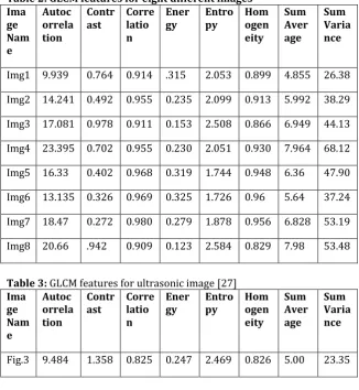
Table 2: GLCM features for eight different images Ima ge Nam e Autoc orrela tion Contr
ast Correlatio n
Ener
gy Entropy Homogen eity Sum Aver age Sum Varia nce
Img1 9.939 0.764 0.914 .315 2.053 0.899 4.855 26.38
Img2 14.241 0.492 0.955 0.235 2.099 0.913 5.992 38.29
Img3 17.081 0.978 0.911 0.153 2.508 0.866 6.949 44.13
Img4 23.395 0.702 0.955 0.230 2.051 0.930 7.964 68.12
Img5 16.33 0.402 0.968 0.319 1.744 0.948 6.36 47.90
Img6 13.135 0.326 0.969 0.325 1.726 0.96 5.64 37.24
Img7 18.47 0.272 0.980 0.279 1.878 0.956 6.828 53.19
Img8 20.66 .942 0.909 0.123 2.584 0.829 7.98 53.48
Table 3: GLCM features for ultrasonic image [27]
Ima ge Nam e Autoc orrela tion Contr
ast Correlatio n
Ener
gy Entropy Homogen eity Sum Aver age Sum Varia nce
Fig.3 9.484 1.358 0.825 0.247 2.469 0.826 5.00 23.35
Image Size of different images taken same of 1024x1024. The table is comparison of GLCM features calculated for eight different images as shown in Fig. 8.
7. CONCLUSION
The analysis work tried to research the employment of GLCM textural parameters as a picture quality metric. The planned technique mentioned the connectedness of radius and angle that happen to be the foremost crucial input parameters in GLCM process. It are often finished that the foremost applicable worth of radius for analysis would be one as closely spaced pixels square measure additional possible to be related than those that square measure spaced distant. The radius that should be utilized in computing the GLCM is also obtained from the autocorrelation performance of the image. The radius worth at that the normalized autocorrelation perform of the image becomes too tiny will function Associate in Nursing edge on the worth which can be used for computing the GLCM. No definite conclusions are often drawn relating to the worth of angle. For many of the studies, it would be applicable to calculate the textural parameters for all the four worth of angle and use the common value. Therefore GLCM happens to be a decent person in finding out completely different pictures but no such claims are often created for image quality. The analysis of the results shows that the textural parameter versus image size might not invariably follow a particular trend for chosen values of radius and angle. Playing thorough process for all attainable radiuses Associate in nursing angle values can be thought-about as a choice so selecting the foremost applicable set of graphs. This but reduces the possibilities of automating the whole method. Therefore it seek for the most effective image quality metric continues.
REFERENCES
[1] Smith,R.A., “Screening women aged 40-49: where are we today?” J Natl Cancer Inst, 1995, pp. 1198-1199.
© 2016, IRJET | Impact Factor value: 4.45 | ISO 9001:2008 Certified Journal
| Page 1128
[3] Arodz, T. Kurdziel, M. Sevre,E.O.D., and Yuen,D.A., “Pattern Recognition Techniques for Automatic Detection of Suspicious-looking Anomalies in Mammograms”, Computer Methods and Programs in Biomedicine, Elsevier, 2005, pp. 135-149. [4] Mavroforakis,M.E.,Georgiou,H.V.,Dimitropoulos, N. Cavouras, D., and Theodoridis, “Mammographic masses characterization based on localized texture and dataset fractal analysis using linear, neural and support vector machine classifiers”, Artificial Intelligence in Medicine, 2006, pp. 145—162
[5] R.M. Haralick, K. Shanmugam, and I. Dinstein,”Textural Features for Image Classification”, IEEE Trans. on Systems, Man and Cybernetics, Vol. SMC-3, pp. 610-621, 1973.
[6] R.M. Haralick and K. Shanmugam, ”Computer Classification of Reservoir Sandstones”, IEEE Trans. on Geo. Eng., Vol. GE-11, pp. 171-177, 1973.
[7] D.C. He, L.Wang, and J. Juibert,”Texture Feature Extraction”, Pattern Recognition Letters, Vol. 6, pp. 269-273, 1987. [8] M. Iizulca, ”Quantitative evaluation of similar images with quasi-gray levels”, Computer Vision, Graphics, and Image Processing, Vol. 38, pp. 342-360, 1987.
[9] R.W. Conners, M.M. Trivedi, and C.A. Harlow,”Segmentation of a High-Resolution Urban Scene Using Texture Operators”, Computer Vision, Graphics, and Image Processing, Vol. 25, pp. 273-310, 1984.
[10] L.H. Siew, R.H. Hodgson, and E.J. Wood,”Texture Measures for Carpet Wear Asessment”, IEEE Trans. on Pattern Analysis and Machine Intell., Vol. PAMI-10, pp. 92- 105, 1988.
[11] R.W. Conners and C.A. Harlow,”A theoretical comparison of texture algorithms”, IEEE Trans. on Pattern Analysis and Machine Intell., Vol. PAMI-2, pp. 204- 222, 1980.
[12] M.M. Trivedi, R.M. Haralick, R.W. Conners, and S. Goh, ”Object Detection based on Gray Level Co-ocurrence”, Computer Vision, Graphics, and Image Processing, Vol. 28, pp. 199-219, 1984.
[13] J.S. Weszka, C.R. Dyer, and A. Rosenfeld, “A comparative Study of Texture Measures for Terrain Classification”, IEEE Trans. on Systems, Man and Cybernetics, Vol. SMC-6, pp. 269-285, 1976.
[14] Joonmi Oh, Sandra I. Woollley, Theodoros N. Arvanitis and John N. Townend “A Multistage Perceptual Quality Assessment for Compressed Digital Angiogram Images”, IEEE Transactions on Medical Imaging, Vol. 20, No. 12, December 2001. [15] Lisboa,P.G., “A review of evidence of health benefit form artificial neural networks”, Neural Networks, 2002, pp. 11-39. [16] K. Bovis and S. Singh. Detection of masses in medical images using texture features. 15th International Conference on Pattern Recognition (ICPR'00), 2:2267, 2000.
[17] Ahmed NI and Chaya P (1349-1353). Segmentation and Classification of Skin Cancer Images.International Journal of Advanced Research in Computer Science and Software Engineering 4(5) 1349- 1353.
[18] Bhuiyan HA, Azad I and Uddin K (2013). Image Processing for Skin Cancer Features Extraction. International Journal of Scientific & Engineering Research 4(2) 1-6.
[19] Dhinagar JN, Celenk M and AkinlarAM (2011). Noninvasive Screening and Discrimination of Skin Images for Early Melanoma Detection. IEEE Journal 3 1-4.
[20] Das N, Pal A and Mazumder S (2013). An SVM based skin disease identification using Local Binary Patterns. IEEE Journal of Third International Conference on Advances in Computing and Communications 208-211.
[21] Elgamal M (2013). Automatic Skin Cancer Images Classification. International Journal of Advanced Computer Science and Applications 4(3) 287-294.
[22] Jaleel AJ, Salim S and Aswin RB (2013). Computer Aided Detection of Skin Cancer. IEEE Journal of International Conference on Circuits, Power and Computing Technologies 1137-1142.
[23] Jayapal P, Manikandan R, Ramanan M, ShiyamSundar RS and Udhaya TS (2014). Skin Lesion Classification Using Hybrid Spatial Features and Radial Basis network. International Journal of Innovative Research in Science, Engineering and Technology 3(3) 10014-10021.
[24] Li L, Clark A and Wang ZJ (2014). A Computer-aided Diagnostic Tool for Melanoma. IEEE Journal of International Conference on Computational Science and Computational Intelligence 4 114-118.
[25] Maglogiannis I (2009). Overview of Advanced Computer Vision Systems for Skin Lesions Characterization. IEEE Journal 13(5) 721-733.
[26] R. M. Haralick, K. Shanmugam and I. Dinstein “Textural features for Image Classification”, IEEE Transactions on Systems, Man and Cybernetics, Vol.3, pp. 610-621, November 1973.
[27] NishthaAttlas, Dr. Sheifali Gupta. “Wavelet Based Techniques for Speckle Noise Reduction in Ultrasound Images”, Int. Journal of Engineering Research and Applications, 2248-9622, Vol. 4, Issue 2( Version 1), February 2014, pp.508-513 [28] Baraldi Andrea and ParmigianniFlavio, “An Investigation of the Textural Characteristics associated with gray level co-occurrence matrix statistical parameters”, IEEE Transactions on Geoscience and Remote Sensing, vol. 33, No. 2, March 1995. [29] JC-M. Wu, and Y-C. Chen,“Statistical Feature Matrix for Texture Analysis”,Computer Vision, Graphics, and Image Processing; Graphical Models and ImageProcessing, Vol. 54, pp. 407-419, 1992.
© 2016, IRJET | Impact Factor value: 4.45 | ISO 9001:2008 Certified Journal
| Page 1129
[31] Mark Nixon & Alberto Aguado, “Feature Extraction and Image Processing”, Linacre House, Jordan Hill, Oxford OX2 8DP, UK,
Second Edition.
[32] Duda, R. O., Hart, P. E. and Stork, D. G. (2001) Pattern Classification. 2nd edition, John Wiley & Sons, Inc. [33] Bishop, C. M. (1995) Neural Networks for Pattern Recognition. Oxford UniversityPress.
[34] Turk, M. and Pentland, A. P. (1991) Eigenfaces for recognition. Journal of CognitiveNeuroscience, 3, 71-86.
[35] D. Comaniciu, P. Meer, “Mean shift: A robust approach toward feature space analysis”, IEEE Trans. on Pattern Analysis and Machine Intelligence, 2002, 24, pp. 603-619
[36] C. Christoudias, B. Georgescu, P. Meer, “Synergism in Low Level Vision”, Intl Conf on Pattern Recognition, 2002, 4, pp. 40190
[37] P. Felzenszwalb, D. Huttenlocher, “Efficient Graph-Based Image Segmentation”, Intl Journal of Computer Vision, 2004, 59 (2)
[38] D. Martin, C. Fowlkes, D. Tal, J. Malik, “A Database of Human Segmented Natural Images and its Application to Evaluating Segmentation Algorithms and Measuring Ecological Statistics”, Intl Conf on Computer Vision, 2001.
[39] R. Unnikrishnan, C. Pantofaru, M. Hebert, “A Measure for Objective Evaluation of Image Segmentation Algorithms”, CVPR workshop on Empirical Evaluation Methods in Computer Vision, 2005.
[40] Arun R, Madhu S. Nair, R. Vrinthavani and RaoTatavarti. “An AlphaRooting Based Hybrid Technique for Image Enhancement”. Online publication in IAENG, 24th August 2011.
[41] Agaian, SOS S., Blair Silver, Karen A. Panetta, “Transform Coefficient Histogram-Based Image Enhancement Algorithms Using Contrast Entropy”, IEEE Transaction on Image Processing, Vol. 16, No. 3, March 2007.
[42] Jinshan Tang Eli Peli, and Scott Acton, “Image Enhancement Using a Contrast Measure in the Compressed Domain”, IEEE Signal processing Letters , Vol. 10, NO. 10, October 2003.