CONTINUOUS HOPFIELD NETWORK AND QUADRATIC
PROGRAMMING FOR SOLVING THE BINARY
CONSTRAINT SATISFACTION PROBLEMS
1
KHALID HADDOUCH, 1*MOHAMED ETTAOUIL and 2CHAKIR LOQMAN
1UFR: Scientific Computing and Computer sciences, Engineering sciences, Faculty of Science
and Technology, University Sidi Mohamed Ben Abdellah Box 2202, Fez, Morocco
2Department of Computer Engineering, Moulay Ismail University, High School of technology, B.
P. 3103, 50000, Toulal, Meknes, Morocco
E-mail: [email protected] , 1*[email protected] , [email protected]
ABSTRACT
Many important computational problems may be formulated as constraint satisfaction problems (CSP). In this paper, we propose a new approach to solve the binary CSP problems using the continuous Hopfield networks (CHN). This approach is divided into three steps: the first concerns reducing the size of the CSP problems using arc consistency technique AC3. The second step involves modeling the filtered constraint satisfaction problems as 0-1 quadratic programming subject to linear constraints. The last step concerns applying the continuous Hopfield networks to solve the obtained 0-1 optimization model. Therefore, the mapping procedure and an appropriate parameter setting procedure about CSP problems are given in detail. Finally, some computational experiments solving the CSP problems are shown.
Keywords: Constraint Satisfaction Problems, Filtering Algorithms, Quadratic 0-1 Programming, Continuous Hopfield Networks, Energy Function.
1. INTRODUCTION
A large number of problems in artificial intelligence and other areas of computer science can be viewed as special cases of the constraint satisfaction problems. Some examples include machine vision, belief maintenance, scheduling, temporal reasoning, graph problems, aircraft conflict, etc.
A constraint satisfaction problem is defined by a set of variables, a finite and discrete domain for each variable and a set of constraints. Each constraint restricts the combination of values that a set of variables may take simultaneously. Solving the CSP problem requires assigning a value for each variable from each domain in such a way that all constraints are satisfied. The task is to find one solution or all solutions. However, the CSP problems are NP-complete problems requiring a combination of heuristics and combinatorial search methods in order to be solved in a reasonable time[12].
A number of different approaches have been developed for solving the constraint satisfaction problems [10], [18], [19], [21]. Some of them use backtracking to directly search for possible
solutions [5], others use consistency techniques to simplify the original problems [3], [4], [24], and some are a combination of these two techniques [2], [5], [13]. Moreover, we proposed different approaches to solve the constraint satisfaction problems. The first one consists of modeling a constraint satisfaction problem as 0-1 quadratic knapsack problem subject to quadratic constraint [6], [7]. The second one is a new model of the binary CSP problem as 0-1 quadratic programming which consists in minimizing the quadratic function subject to linear constraints[8]. The later model will be used in order to determine a generalized energy function for the binary constraint satisfaction problem. This step is the most important one for solving any binary CSP problem using continuous Hopfield networks.
ISSN: 1992-8645 www.jatit.org E-ISSN: 1817-3195
that all these problems can be reformulated as constraint satisfaction problems [15], [16], [21]. In this paper, we propose a general approach for solving the binary constraint satisfaction problems using the continuous Hopfield networks, which will be able to solve all problems that can be modeled in terms of constraint satisfaction problems.
This paper is organized as follows: In section 2, the arc-consistency procedure used in this approach is studied and the model of the binary CSP problems is formulated as a quadratic assignment problem with linear constraints. In section 3, a generalized energy function associated with the CSP problems is defined and a direct parameter setting procedure is computed. The proposed algorithm is described in the next section. Implementation details of the proposed approach, complexity analysis, and experimental results are presented in the last section.
2. REDUCING THE SIZE OF THE CSP
PROBLEMS AND MODELING THEM
In general, a constraint satisfaction problem forms a class of models representing problems that have common properties, a set of variables and a set of constraints [21]. The variables should be instantiated from a discrete domain while making sure the constraints are satisfied. This study of CSP problems has become focused on binary constraint satisfaction problems i.e., the CSP with constraints of arity less than or equal to 2, and each constraint Cij between variables yi and yj is defined by its
binary relation Rij. Formally speaking, the binary
constraint satisfaction problems are defined by triple sets (Y,D, C) where:
- Y = {y1,...,yN} is a set of N variables,
- D = {D(y1),...,D(yN)} where each D(yi) is a
set of di possible values for yi,
- C = {Cij} is a set of m constraints which
restricts the values that the variables yi and yj
can simultaneously take.
The solution of constraint satisfaction problems is obtained by assigning each variable a value from its domain satisfying all constraints [10]. In order to use the continuous Hopfield networks for solving the constraint satisfaction problems, we opted for using the mathematical model which consists in modeling the CSP problems as a 0-1 quadratic programming. This model can be used to define the generalized energy function of the CHN. However,
before modeling the CSP problems, we can use the arc consistency technique in order to reduce the size of the CSP problems and, thus, reduce the continuous Hopfield network architectures.
2.1 Consistency techniques
In general, a binary constraint satisfaction problem is represented as an undirected graph with the vertices corresponding to the variables and the edges corresponding to the constraints. It is known that, the binary CSP problems have only two kinds of constraints: unary constraints and binary constraints. The simplest degree of consistency that can be enforced on a CSP problem is node consistency which concerns only the unary constraints [10]. However, a stronger degree of consistency is arc consistency. The latter concerns the binary constraints in CSP problem and guarantees that each value admits at least a support in each constraint. Many algorithms have been proposed to establish arc consistency such as AC1, AC2,...,AC2000 and AC3.1[3], [4], [23], [24].
Definition 1
Let Cij a binary constraint between two
variables yi and yj, with two domains D(yi) and
D(yj).
We call Cij arc consistent if
- ∀ a ∈ D (yi}), ∃ b ∈ D(yj) such that (a, b)
satisfies the constraint Cij ,
- ∀ b ∈ D (yj}), ∃ a ∈ D(yi) such that (a, b)
satisfies the constraint Cij} .
We call a CSP problem arc consistent if all its binary constraints are arc consistent.
The description of the arc consistency AC3 technique which was used is the following [19]: Initially, all arcs (Cij,yi) are put in a set named K.
Then, each arc is revised in turn, and when the revision is effective (at least one value has been removed), the set K has to be updated. This revision removes values of D(yi) that have become
inconsistent with respect to constraint Cij [19]. The
algorithm is stopped when the set K becomes empty. Therefore, the property of consistency is forced for CSP problem.
the model of the CSP problems. In this context, there are three important roles of this filtering:
- Prove that the CSP problems do not admit a solution (if one domain after filtering is empty)[10].
- Reduce the size of the modeled CSP problems since for each value from variables'domains is associated with the binary variable. Therefore, if any inconsistent value from the variables'domains is deleted, the represented binary variable must be eliminated from the proposed model and, thus reduce the size of this model as much as possible.
- Reduce the Hopfield neural network architectures. When we reduce the size of this model, the number of neurons in the architecture of the continuous Hopfield networks is reduced because each binary variable is associated with one neuron in the continuous Hopfield networks.
2.2 Modeling The Constraint Satisfaction Problems
The constraint satisfaction problems have been recognized as an efficient model for solving many combinatorial and complex problems. These problems are formulated as 0-1 quadratic knapsack problem subject to quadratic constraint [6],[7]. Another model of the CSP problem as 0-1 quadratic programming, which consists of minimizing a quadratic function subject to linear constraints, has been proposed [8].
In the following, we want to present the proposed model of the binary constraint satisfaction problems. For each variable yi of the CSP problem,
we introduce di binary variables xik such that:
1 =
= ( )
0
i k
ik k i
if y v
x v D y
Otherwise
∈
(1)
Where k∈{1,...,di},i∈{1,..., }N
This matrix is easily converted to a n-vector:
(
11 11 1)
=
T
d N NdN
x
x
x
x
x
with
=1
= Ni i
n
∑
d and di =|D y( ) |iBased on this notion of encoding values for each variable, we can define the objective function and the constraints of our model.
2.2.2 Objective function
Each constraint Cij between two variables yi and yj is defined by its relation Rij (Rij is a subset
of the cartesian product D y( )i ×D y( j), specifying
the compatible values between yi and yj). Note
that, if there is no constraint between variables yi andyj, R v vij( ,r s) holds for any pair ( ,v vr s) of
( )i ( j)
D y ×D y . For each couple ( ,v vr s) such that
( ,v vr s)∈Rij, we generate a constraint:
= 0 ir js
x x (2) For each relation Rij , the constraints (2) can be
aggregated in a single constraint:
=1 =1
= 0 d
di j
irjs ir js r s
q x x
∑∑
(3)Where = 1 ( , ) 0
r s ij
irjs
if v v R
q
Otherwise
∈
and i∈{1,..., },N j∈{1,..., }, <N i j These constraints (3) can be aggregated in a single constraint:
=1 =1 < =1 =1
( ) = = 0
d d j
N N i
irjs ir js i j i j r s
f x
∑ ∑ ∑∑
q x x (4)The later constraint can be writing in the following form:
=1 =1 =1 =1
1
( ) = = 0
2
d d j N N i
irjs ir js i j r s
f x
∑∑∑∑
q x x (5)Where:
If i<j then = 1 ( , )
0
r s ij
irjs
if v v R
q
Otherwise
∈
If i=j then qirjs = 0 ∀ ∈r {1,...,di} and
{1,..., j}
s d
∀ ∈ ,
If >i j then qirjs =qjsir,
If there is no constraint between variables yi and yj then qirjs= 0 ∀ ∈r {1,...,di} and
{1,..., j}
s d
∀ ∈ .
Finally, we can define the objective function
( )
f x in the following way:
1 ( ) =
2 T f x x Qx
ISSN: 1992-8645 www.jatit.org E-ISSN: 1817-3195
2.2.3 Constraints
Each variable yi must take a unique value from its domain D y( )i , then the linear constraints of the CSP problem are defined bellow:
=1
= 1 {1,...., } di
ik k
x ∀ ∈i N
∑
(6) The later constraints can be written in the following matrix form:Ax=b
Finally, we obtain the following 0-1 quadratic program (QP) with a quadratic function subject to linear constraints:
1 ( ) =
2 ( )
= {0,1}
T
n
Min f x x Qx
Subject to QP
Ax b
x
∈
Where Q is an n n× symmetric matrix, A is an N×n matrix and b is an N vector.
The following theorem establishes the links between the binary CSP problems and an optimization model QP.
Theorem 1 [8]
Let V(QP) an optimal value of the 0-1 quadratic programming (QP). The value V(QP) is equal to zero if and only if the binary constraint satisfaction problem has a solution.
In this work, our objective is to solve the constraint satisfaction problems using the continuous Hopfield networks. Then, in this case, the most important step consists of representing or mapping the constraint satisfaction problems in the form of the energy function associated with the continuous Hopfield networks. According to the proposed model, which consists of modeling the constraint satisfaction problems into a quadratic programming QP problem, we define the associated energy function and the parameters setting. Therefore, the continuous Hopfield networks can be used to solve the binary constraint satisfaction problems.
3. CONSTRAINT SATISFACTION
PROBLEMS SOLVED BY CONTINUOUS HOPFIELD NETWORKS
As can be noticed, after filtering the constraint satisfaction problems via the arc consistency algorithm AC3, we can model it (filtered CSP problems) into 0-1 quadratic programming with a quadratic function subject to linear constraints. Based on this model, we present a general method for solving the CSP problems using the continuous Hopfield networks.
In the beginning of the 1980s, Hopfield published two scientific papers, which attracted a lot of interest. This was the starting point of the new area of neural networks, which continues today. In the same context, Hopfield and Tank presented the energy function approach in order to solve several optimization problems [17]. Their results encouraged a number of researchers to apply this network for solving different problems [1], [17], [27].
The continuous Hopfield neural network is a generalization of the discrete case. Afterwards, many researchers implemented continuous Hopfield network to solve the optimization problem, especially in mathematical programming problems. Then, the continuous Hopfield network is a major artificial neural network for solving optimization problems [27].
As we know, the CHN is a fully connected neural network i.e. the n neurons of Hopfield network are fully connected. Let Wij be the strength of the
connection from neuron i to neuron j. Each neuron i has an offset bias. The current state and the output of the neuron i are respectively represented by ui
and xi [26]. The dynamics of the CHN is described
by the differential equation:
du = u b Wx i
dt − +τ + (7) Where u, x and ib will be the vectors of neuron states, outputs and biases. In the continuous Hopfield networks, the relationship between the internal state ui of a neuron i and its output level
i
x is determined by an activation function, which is bounded below by 0 and above by 1. Commonly, this activation function is given by:
0
0
1
= ( ) = (1 tanh( )) > 0
2
i
i i
u
x g u u
u
+ (8)
activation function. The proof of stability of such continuous Hopfield networks relies upon the fact that E x( ) is a Lyapunov function, provided that the
inverse function of g u,( ) (the first derivative of the activation function), exists. The existence of this equilibrium points for the CHN is guaranteed if a Lyapunov function exists. Hopfield proposed an energy function of the continuous Hopfield network that, if matrix W is symmetric [14], then the following Lyapunov function exists:
1 0 =1 1 1 ( ) = ( ) ( ) 2 n x i
T b T
i
E x x Wx i x g z dz
τ
−
− − +
∑∫
(9)Where the function g−1( )z is a monotone
increasing function. The idea is that the networks Lyapunov function, when τ† ∞, is associated with the cost function to be minimized in the combinatorial problem. In this way, the CHN output can be used to represent a solution of the combinatorial problem. Then, for solving any combinatorial problem via the continuous Hopfield networks, we will write this problem in the following form:
1
( ) = ( )
2
T b T
E x − x Wx− i x (10)
Typically, in the CHN, the energy function is made equivalent to the objective function which is to be minimized, while each of the constraints of the optimization problem are included in the energy function as penalty terms.
3.1 Generalized Energy Function For The Constraint Satisfaction Problems
In order to solve the constraint satisfaction problems using the continuous Hopfield networks, we define the generalized energy function for the CSP problems basing on the proposed model. Recall that, the constraint satisfaction problems are modeled as 0-1 quadratic programming with n variables and N linear constraints [8].
1 ( ) = 2 ( ) = {0,1} T n
Min f x x Qx
Subject to QP Ax b x ∈
The generalized energy function allows representing mathematical programming problems with quadratic objective function and linear constraints. This energy function includes the objective function f x( ) and it penalizes the linear constraints Ax=b with a quadratic terms and a
linear terms. Then, the generalized energy function must also be defined by [27]:
( ) = O( ) C( ) [0,1]n
E x E x +E x ∀ ∈x (11) Where:
- O( )
E x is directly associated with the objective function of the constraint satisfaction problems,
- EC( )x is a quadratic function that penalizes the violated constraints of the CSP problems.
The following generalized energy function is proposed:
1
( ) = ( ) ( )
2 2
T T
E x α x Qx+ Ax Φ Ax
+x diagT ( )(1γ − +x) βTAx (12)
Where α∈R+, β∈RN, γ∈Rn, Φ is an N×N symmetric matrix and diag( )γ denotes the diagonal matrix constructed from the vector γ .
To define the energy function for the CSP problems, the following considerations need to be taken into account so that the mathematical expression of energy function (12) is simplified. Only the main diagonal terms of the quadratic matrix parameter Φ are considered:
0 =
= kj
if j k
if j k
φ
≠
Φ
Where φ is a scalar, All linear constraints are equally weighted, where β is the associated parameter, The parameter penalizing the non-extreme values of xir is γ . We notice that the CSP problems have only one family of linear constraints:
=1
( ) = = 1 {1,..., } di
i ik
k
e x
∑
x ∀ ∈i N (13)Consequently, the following generalized energy function for the CSP problems is proposed:
2 =1 =1 1 ( ) = ( ) ( ( )) ( ) 2 N N i i i i
E x αf x + φ
∑
e x +β∑
e x=1 =1 (1 ) d N i ir ir i r x x γ
+
∑∑
− (14)which in algebraic form is:
, =1 =1 =1 =1 =1 =1
1 ( ) =
2 2
d
d j d d
N i N i i
irjs ir js ir is
i j r s i r s
ISSN: 1992-8645 www.jatit.org E-ISSN: 1817-3195
=1 =1 =1 =1
(1 )
d d
N i N i
ir ir ir
i r i r
x x x
β γ
+
∑∑
+∑∑
− (15)In our case, the weights Wirjs of the continuous Hopfield networks are in function of the coefficients corresponding to the quadratic terms
ir js
x x , and the external inputs iirb (thresholds) are in function of the coefficients corresponding to the linear terms xir in the chosen energy function. Then to determine the weights and thresholds, we use the assimilation between equation (10) and the algebraic form of the generalized energy function. Finally, the weights and thresholds of the connections between the n neurons are:
= (1 ) 2
=
irjs ij irjs ij ij rs
b ir
W q
i
α δ δ φ δ δ γ
β γ
− − − +
− −
(16)
Where δij is the Kroenecker delta.
1 =
= 0 ij
if i j
if i j
δ ≠
In this way, the quadratic programming has been presented as an energy function of continuous Hopfield networks. To solve an instance of the CSP problem, the parameter setting procedure is used. This procedure assigns the particular values for all parameters of the network, so that any equilibrium points are associated with a valid affectation for all variables when all constraints are satisfied.
3.2 Parameters Setting Of The Continuous Hopfield Networks
The weights and thresholds of the continuous Hopfield network depend on the parameters α, φ,
β and γ. To solve the CSP problems via the CHN, an appropriate setting of these parameters is needed. In this subsection, our objective is to determine these parameters. The dynamics of the CHN must ensure that any invalid solution x∈HF cannot be a stable point. Any constraint which is imposed on the dynamics of the CHN must be translated into a set of constraints on its parameter values, this is the kernel of the parameter setting. A feasible solution is guaranteed by the CHN from a stability analysis of the Hamming hypercube corners set:
= { : {0,1} }n C
H x∈H x∈
Where H= {x∈[0,1] }n is the Hamming hypercube and HF = {x∈HC:Ax= }b is a set of feasible solutions.
The parameter setting procedure is based on the partial derivatives of the generalized energy function:
( )
= ir( )
ir E x
E x x
∂ ∂
Where:
=1 =1 =1
( ) = (1 2 )
dj d
N i
ir irjs js is ir
j s s
E x α
∑∑
q x +φ∑
x + +β γ − x (17)A point x∈H will be an equilibrium point for the CHN if and only if the two following relations are satisfied [27]:
( ) 0 = 0 ( ) 0 = 1
ir ir
ir ir
E x if x
E x if x
≥
≤
(18)
Where ∀ ∈i {1,..., }N and ∀ ∈r {1,...,di}
This procedure uses the hyperplane method [27], so that the Hamming hypercube H is divided by a hyperplane containing all feasible solutions. To avoid the stability of any no feasible and corner solution x∈HC−HF, the following instability conditions are imposed:
( ) = 0
( ) = 1
ir ir
ir ir
E x if x
E x if x
ε ε
≤ −
≥
(19)
Based on this hyperplane method and the associated half-spaces, the complementary corners set of the feasible solutions for the CSP problem is partitioned and a set of analytical equations of the CHN parameter is proposed. The hyperplane method is briefly explained below; however, for simplicity reasons the following parameters constrains are first assigned:
- To minimize the objective function, we impose the following constraint: α > 0,
- On the other hand, to penalize the non-feasibility of the family of linear constraints
( ) i
e x , it is natural to impose the following constraint: φ≥0,
- In order to guarantee the instability of the interior points x∈ −H HC, some initial conditions are imposed on some parameters:
Wirir=− +φ 2γ ≥0 (20)
Where i∈{1,..., },N r∈{1,...,di}.
Given the linear constraints of the QP problem:
( ) = 1 {1,..., }
i
1,1 1,2
=
C F
H −H H
HThis two partition are defined in the folowing way:
1,1 0
- H = {∃i e x: ( ) > 1} { ( )i
e x ≥N}where 0
=1
( ) = iN i( )
e x
∑
e x . In this case, one variablei
y has been assigned two different values v vr, s in
( )i
D y so that xir =xis = 1. Consequently, the
following instability condition is imposed:
( ) 2
ir
E x ≥ φ β γ ε+ − ≥ (22)
1,2 0
- H = {∃i e x: ( ) < 1} { ( ) <i
e x N}In this case, one variable yi has not been assigned any value vr∈D y( )i , such that
= 0 {1,..., }
ir i
x ∀ ∈r d . Therefore, the following instability condition is imposed:
( ) ir
E x ≤αd+ + ≤ −β γ ε (23)
With
=1 =1
=
dj N
irjs j s
d Max q
∑∑
Then, we can determine the parameters setting by resolving the following system:
> 0 , 0
2 0 (24. )
2 = (24. )
= (24. )
a b
d c
α φ
φ γ
φ β γ ε
α β γ ε
≥
− + ≥
+ −
+ + −
The inequation (24.a) guaranteed the satisfaction of the integrity constraints (xir∈{0,1}), but the
equations (24.b) and (24.c) guaranteed the satisfaction of the linear constraints. These parameters setting are determined by fixing α , ε and computing the rest of parameters ,γ β and φ:
=d 2
φ α+ ε, γ φ= / 2 β ε= −3γ Then, the weights and thresholds of continuous Hopfield networks (system 16) can be computed using these parameters setting. Finally, we obtain an equilibrium point for the CHN using the algorithm depicted in [26], so compute the solution of constraint satisfaction problem.
4. DESCRIPTION OF THE NEW SOLVER
OF CSP PROBLEMS
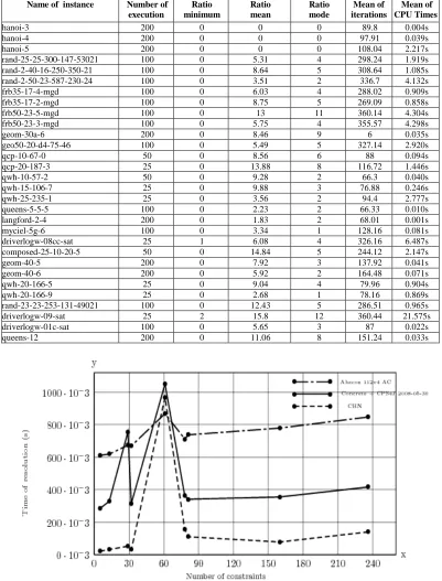
[image:7.612.334.542.121.483.2]The new solver was developed to find a solution of the CSP problem via the continuous Hopfield networks. The diagram of this algorhitm is described by the following steps (Figure 1):
Figure 1: Diagram of the proposed algorithm
The important steps of this algorithm are the following:
- The first step is to read the data of CSP problem, this data is presented in XML file (database). This reading requires developing techniques to extract data (domains, variables, relationships and constraints).
- The main objective of the second step is to filter the CSP problem. There are two important roles of this filtering:
• Reducing the size of the CSP problem,
• Showing that the CSP problem does not admit a solution (if one domain after the filter is empty).
Modeling the filtered CSP Input data of CSP problem
Filtering CSP via AC3
∃ i∈{1, …, N} D(yi) = ∅
No Yes
Yes
V(QP) = 0 No Solution not find
No Solution End
End Solution CHN(Wij, iib)
ISSN: 1992-8645 www.jatit.org E-ISSN: 1817-3195
This filtering is realized by the arc consistency technique AC3.
- The third step concerns modeling the filtered CSP problem as 0-1 quadratic programming (determining the matrix Q, the matrix A and the vector b).
- The last step concerns using the CHN to obtain a solution of this model, so that if an optimal value of the 0-1 quadratic programming is equal to 0 (V(QP) = 0), the solution of CSP problem is found; else, the CSP problem has no solution (theorem 1).
5. COMPUTATIONAL EXPERIMENTS
In order to show the practical interest of the proposed approach, the experiments and the complexity analysis are studied in this section.
5.1 Complexity analysis
In this subsection we evaluate and determine the complexity of arc consistency algorithm (AC3) and the continuous Hopfield network algorithm. Given a constraint satisfaction problem with N variables, m constraints and dmax the size of the largest domain. The complexity of the AC3 algorithm is on the order of ( 3 )
max
O md average time complexity [20]. Simulating the continuous Hopfield network algorithm for large instances of constraint satisfaction problems constitutes real challenges in terms of the memory space that must be allocated for the weight matrix W and thresholds vector ib, which is the highest-cost data structure. In general, the number of memory bytes required and the time complexity of simulating the continuous Hopfield networks are studied in detail in the following work [25].
5.2 Numerical results
The experiment aims at solving problems of different natures (random, academic and real-world problems). These series represent a large spectrum of instances (benchmarks). These experiments are executed in personal computer with a 2.79 GHz processor and 512 MB RAM. The performance has been measured in terms of the CPU time per second.
5
1
= 0.999 i 10
ik
i
d k
x U
d
− + − +
Where i= 1,...,N k, = 1,...,di and U is a random uniform variable in the interval [ 0.5, 0.5]− . Recall that, N is the number of variables. Based on
a series of the experiments, α and ε are fixed by the following values:
1 =
N
α , 4
= 10
ε − .
The rest of parameters setting ,γ β and φ are computed:
=d 2
φ α+ ε, γ φ= / 2 and β ε= −3γ . In our experimentation, some instances to be solved were chosen from the library benchmarks[21], are used to test this software.
A statistical study was performed in order to study the quality of our approach. This study is based on the calculation operator’s performance:
- Ratio mode: the most repetitive (mode) optimal value obtained by CHN in number of run,
- Ratio mean: the average of the optimal value in a number of run,
- Ratio minimum : the smaller optimal value (better results obtained by our solver),
- Mean of CSP time: the average time consumed to obtain the solution in a number of run.
In this context, for each instance, if the minimum ratio is equal to 0, then the proposed approach has found the solution. Otherwise, the proposed approach has not found a solution.
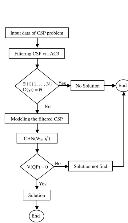
The simulation results are presented in Table (1). Compared with other CSP solvers, the time resolution obtained by our approach is better than others, it does not exceed a few seconds in most cases.
We also compared our results with those given by two different solvers Abscon [29] And Concrete [30]. These results show that the continuous Hopfield network is an effective tool for solving constraint satisfaction problems. In general, our approach is largely effective; it can obtain a solution in a minimum time for most instances (Figure 1).
6. CONCLUSION
problems after converting the latter into binary CSP problems [22]. The experimental results show that our method can find a good optimal solution in a short time. Several directions can be investigated to try to improve this method such as reducing the
architecture of Hopfield neural networks [9]. Other studies are in progress to apply this approach to many real-world problems such as aircraft conflict, timetabling and recognition.
TABLE 1:Computational Result Of The Typical CSP Instances
Name of instance Number of execution
Ratio minimum
Ratio mean
Ratio mode
Mean of iterations
Mean of CPU Times
hanoi-3 200 0 0 0 89.8 0.004s
hanoi-4 200 0 0 0 97.91 0.039s
hanoi-5 200 0 0 0 108.04 2.217s
rand-25-25-300-147-53021 100 0 5.31 4 298.24 1.919s
rand-2-40-16-250-350-21 100 0 8.64 5 308.64 1.085s
rand-2-50-23-587-230-24 100 0 3.51 2 336.7 4.132s
frb35-17-4-mgd 100 0 6.03 4 288.02 0.909s
frb35-17-2-mgd 100 0 8.75 5 269.09 0.858s
frb50-23-5-mgd 100 0 13 11 360.14 4.304s
frb50-23-3-mgd 100 0 5.75 4 355.57 4.298s
geom-30a-6 200 0 8.46 9 6 0.035s
geo50-20-d4-75-46 100 0 5.49 5 327.14 2.920s
qcp-10-67-0 50 0 8.56 6 88 0.094s
qcp-20-187-3 25 0 13.88 8 116.72 1.446s
qwh-10-57-2 50 0 9.28 2 66.3 0.040s
qwh-15-106-7 25 0 9.88 3 76.88 0.246s
qwh-25-235-1 25 0 3.56 2 94.4 2.777s
queens-5-5-5 100 0 2.23 2 66.33 0.010s
langford-2-4 200 0 1.83 2 68.01 0.001s
myciel-5g-6 100 0 3.34 1 128.16 0.081s
driverlogw-08cc-sat 25 1 6.08 4 326.16 6.487s
composed-25-10-20-5 50 0 14.84 5 244.12 2.147s
geom-40-5 200 0 7.92 3 137.92 0.041s
geom-40-6 200 0 5.92 2 164.48 0.071s
qwh-20-166-5 25 0 9.04 4 79.96 0.904s
qwh-20-166-9 25 0 2.68 1 78.16 0.869s
rand-23-23-253-131-49021 100 0 12.43 5 286.51 0.965s
driverlogw-09-sat 25 2 15.8 12 360.44 21.575s
driverlogw-01c-sat 100 0 5.65 3 87 0.022s
queens-12 200 0 11.06 8 151.24 0.033s
[image:9.612.106.507.175.702.2]ISSN: 1992-8645 www.jatit.org E-ISSN: 1817-3195
REFERENCES
[1] A. AKOUM, B. DAYA and P. CHAUVET “Two neural networks for license number plates recognition”, Journal of Theoretical and
Applied Information Technology, Vol. 12, No.
1, 2010, pp. 25-32.
[2] F. Bacchus and A. Grove, “On the Forward Checking algorithm. In Principles and Practice of Constraint Programming, ” Springer-Verlag, New York, Vol. 976, 1995, pp. 292–309. [3] C. Bessière and J-C. Régin, “Refining the basic
constraint propagation algorithm,” In proceedings of the Seventeeth International Joint conference on Artificial Intelligence (IJCAI’), 2001, pp. 309–315.
[4] C. Bessière, “Arc-consistency and arc-consistency again,” ArtificialIntelligence, Vol. 65, No. 1, 1994, pp. 179–190.
[5] R. Dechter and D. Frost, “Backtracking algorithms for constraint satisfaction problems,” Constraints, International Journal, 1998.
[6] M. Ettaouill, “A 0-1 quadraric knapsack problem for modelizing and solving the constraint satisfaction problem,” in Lecture Notes in Artificial Intelligence N°1323, Springer Verlag, Berlin, 1997, pp. 61–72.
[7] M. Ettaouill and C. Loqman, “Constraint Satisfaction Problems Solved by Semidefinite Relaxations,” WSEAS TRANSACTIONS on
COMPUTERS, Vol. 7, No. 7, 2008, pp. 951–
961.
[8] M. Ettaouill and C. Loqman, “A New Optimization Model for Solving the Constraint Satisfaction Problem,” Journal of Advanced Research in Computer Science, Vol. 1, No. 1, 2009, pp. 13–31.
[9] M. Ettaouill and Y. Ghanou, “Neural architectures optimization and genetic algorithms,” WSEAS TRANSACTIONS on
COMPUTERS, Vol. 8, No. 3, 2009, pp. 526–
537.
[10]M. Ettaouil, K. Haddouch and C. Loqman, “Quadratic programming and genetic algorithms for solving a Constraint Satisfaction Problems (CSP)”, JOURNAL OF
COMPUTING, Vol. 4, No. 4, APRIL 2012, pp.
43-52.
[11]A. Ghosh and all., “Object background classification using Hopfield type neural network,” International Journal of Pattern Recognition and Artificial Intelligence, Vol. 6, No. 5, 1992, pp. 989-1008.
[12]R. M. Haralick and G. L. Elliott, “Increasing tree search efficiency for constraint satisfaction problems,” Artificial Intelligence, Vol. 14, 1980, pp. 263–313.
[13]J. J. Hopfield, “Neural networks and physical systems with emergent collective computational abilities,” Proceedings of the National Academy of Sciences of the United States of America, Vol. 79, 1982, pp. 2554–2558.
[14]J. J. Hopfield and D.W. Tank, “Neural computation of decisions in optimization problems,” Biological Cybernetics, Vol. 52, 1985, pp. 1–25.
[15]S. Hosseini, K. Zamanifar, “Using a Conflict-Based Methed to Solve Distributed Constraints Satisfaction Problems,” Journal of Theoretical
and Applied Information Technology, Vol. 5,
No. 4, April 2009, pp. 446-463.
[16]A. Idrissi, “Some methods to treat capacity allocation problems”, Journal of Theoretical
and Applied Information Technology, Vol. 37
No.2, 31March 2012, pp. 141-158.
[17]D. Kaznachey, A. Jagota and S. Das, “Neural network-based heuristic algorithms for hypergraph coloring problems with applications,” Journal of Parallel and Distributed Computing, Vol. 63, No. 9, 2003, pp. 786-800.
[18]V. Kumar, “Algorithms for Constraint Satisfaction Problems: A Survey,” AI Magazine, Vol. 13, No. 1, 1992, pp. 32–44. [19]C. Lecoutre, F. Boussemart and F. Hemery,
“Revision ordering heuristics for the Constraint Satisfaction Problem,” 1st International Workshop on Constraint Propagation and Implementation (CPAI’04), 2004, pp. 9–43. [20]C. Lecoutre, “Benchmarks in XCSP 2.1 XML
representation of CSP/WCSP/QCSP instances,” Available at http://www.cril.univ-artois.fr/lecoutre/research/benchmarks/benchma rks.html, 2008.
[21]C. Lecoutre, “Constraint Networks: Techniques and Algorithms,” ISTE/Wiley, 2009.
[22]N. Mamoulis and K. Stergiou, “Solving non-binary CSPs using the Hidden Variables Encoding,” In Proceedings of CP’ (2001). [23]AK. Marckworth, “Consistency in networks of
relations,” Artificial Intelligence, Vol. 8, 1977, pp. 99–118.
[25]G. Serpen, “Managing spatio-temporal complexity in Hopfield neural network simulations for large-scale static optimization,”
Mathematics and Computers in Simulation,
Vol. 64, 2004, pp. 279–293.
[26]P.M. Talaván and J. Yáñez, “A continuous Hopfield network equilibrium points algorithm,” Computers and Operations Research, Vol. 32, 2005, pp. 2179–2196.
[27]P.M. Talaván and J. Yáñez, “The quadratic assignment problem. A neuronal network approach,” Neural Networks, Vol. 19, No. 4, 2006, pp. 416-428.
[28]H. Shouval and all., “An all-optical Hopfield network: theory and experiment. A neuronal network approach,” International Journal of Neural Systems, Vol. 1, No. 4, 1991, pp. 355– 360.
[29]“CSP 2008 Competition: benchmarks results per solver Result page for solver Abscon 112v4 AC, ” Available at http://www.cril.univ-artois.fr/CPAI08/results/solver.php?idev=15&i dsolver=363, 2008.
[30]“CSP 2008 Competition: benchmarks results per solver Result page for solver Concrete + CPS4J 2008-05-30”, Available at