PLACEMENT AND SIZING OF DISTRIBUTED GENERATORS IN DISTRIBUTED NETWORK BASED ON LRIC AND LOAD GROWTH CONTROL

(1)

ISSN: 1992-8645 www.jatit.org E-ISSN: 1817-3195

355

LC FEATURES COMBINED CHIRPLET TRANSFORM AND

FRACTAL THEORY ON HIGH VOLTAGE INSULATORS

1_{ALI HUI,} 2_{HUI LIN}

1_{Department of Electrical and Control Engineering, Xi’an University of Science and Technology, Xi’an}

710054, Shaanxi, China

2_{Department of Automation, Northwest Polytechnical University, Xi’an 710076, Shaanxi, China}

ABSTRACT

The voltage grade of electrical transmission line is getting higher and higher, consequently, flashover of transmission insulators is getting more and more severe in high-voltage (HV) and ultra-high-voltage (UHV) systems under serious pollutions, which menaces the safety of power transmission system heavily. The crux to enhance the security of power system is to discover ways of monitoring states of insulator’s surface by some eigenvalues. A new method, combined chirplet transform with fractal theory, was proposed in this paper, and is taken as the ruler to define fractal dimension, which is used to describe characteristics of signals. Chirplet-fractal dimension is defined as the sum of residues of decomposed signals. The fractal characteristics of leakage current during flashover are obtained from this dimension. The results show that the chirplet-fractal dimension efficiently describes the information of arcs discharge in LC, and it is also a good eigenvalue for flashover discrimination and risk prediction.

Keywords: Fractal Dimension, Chirplet Transform, Non-stationary Signal, Leakage Current, Flashover

1. INTRODUCTION

As high-voltage (HV) and ultra-high-voltage (UHV) transmission lines have been used more and more widely, flashovers from contaminated insulators became the primary factor threatening the reliability of HV transmission system, and the harm from pollution flashover has surpassed the thunder impact by far[1]. At present, the most universal actions for preventing pollution flashover are regular cleaning, using antipollution material, and adjusting creepage distance. However, these methods have obvious defects such as waste of resources, blindness, and so on, which are resulted from the lack of accurate understanding of insulator surface condition. The key to improve the security of power system is to explore resultful methods of monitoring states of insulator’s surface by some eigenvalues. Thus, it is important to choose an efficient eigenvalue.

At present, leakage current (LC) is the best discrimination standard with practical significance, because it generally reflects the voltage, the climate and the contamination. LC is a token of descending degree of insulation level, and is easier to supervise than other values, such as surface electric field, voltage distribution, infrared image[1].The study of LC is mainly focused on its maximum value, phase angle, different quantities of pulse and frequency features[2-4], but results express obvious different

among them[5]. Since supervised LC, including disturbs and noise signals because of complex local environment and atrocious weather, is non-stationary random signal, it is vital to analyze LC with effective method.

In this paper, a new idea is proposed to use fractal to describe chirplet transform results of signals. It integrates chirplet transforms with fractal geometry, namely chirplet-fractal dimension. This dimension describes the change rule of the sum of residues from decomposed signals. The fractal characteristics of LC are calculated with chirplet-fractal dimension, and LC is obtained from artificial pollution test.

2. FRACTAL DIMENSION

2.1Box Dimension

(2)

356 and to describe the common structure of a great kind of irregular sets and functions that cannot be described by traditional Euclidean geometry and calculus method.

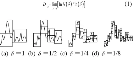
In fractal theory, fractal dimension is a significant parameter to depict fractal phenomenon, and it is the further development of traditional dimensions. Fraction describes the degree and complicacy of the fractal collection to fill space. Since the birth of fractal dimension, more than ten kinds of different fractal dimensions have been defined in allusion to different objects, for example, box dimension, Hausdorff dimension, similarity dimension, information dimension, and correlation dimension, and so on [6,7]. Among these dimensions, box dimension is the easiest and most widely used. As shown in figure 1, the box

dimension of a set S with n-dimension is defined

as follows: for any δ >0 , let N( )δ be the

minimum number of n-dimension cubes of

side-lengthδ needed to coverS. The box dimension D_B

of S[8] is:

( ) ( )

[

]

0

lim ln / ln

B

D N

δ→ δ δ

= (1)

The ideal fractal has infinite details. However, fractal phenomenon in nature generally doesn’t have fractal characteristic on condition of finite scale, so box dimension cannot be calculated by equation (1). The approximate method is usually used to compute it in practice, viz. take ruler, with

certain length,

∆

as the minimum (or maximum)

side-length of meshes, then magnify (or minify)

them to k∆ ∈,k z+,k<N₀ step by step, note N_k∆

as the number of meshes that cover S in

side-length of k∆, and N_k∆is shown as:

0/

1

{max{ [( 1) 1: ]}

min{ [( 1) 1: ]} / }

N k

k j

N ceil x j k jk

x j k jk k

∆ =

= − +

− − + ∆

∑

₍₂₎

where ceil y( ) takes integer upward, namely

( ) 1

ceil m+δ = +m

.

The famous Richardson plot[7] depicts the curve

of lnk∆~ lnNk∆ , as shown in figure 2. This

figure can be divided into three regions A, B and

C in terms of different slopes of the curve. k∆ is

very small in region A, and fractals in nature generally doesn’t have scale-free self-similarity.

At the same time, k∆ is too large to reflect

details of the curve in region C . So region

Bwith preferable linearity is commonly regarded

as the scale-free region. Suppose the start point

and the end point of this region are k₁and k₂,

respectively, then lnk∆~ lnN_k_∆ satisfies linear

regress model,

1 2

lnNk∆= −DBlnk∆ +b, k ≤ ≤k k (3)

where D_B is the slope of the curve in region Band

is defined as box dimension.

2.2Chirplet-fractal Dimension

According to the definition of wavelet transform, radix function package, changed by translating and

dilating mother wavelet ψ( )t , is:

( )

1/ 2

( )

, / , , 0

a b t a t b a b R a R a

ψ ₌ − ψ_ ₋ _ _∈ _∈ + _≠

  (4)

[image:2.612.325.523.344.502.2]

(a)δ＝1 (b) δ＝1/2 (c) δ＝1/4 (d) δ＝1/8

Figure 1: Definition Of Box Dimension

C

A

B

1

lnk∆ lnk2∆ lnk∆

lnNk∆

[image:2.612.93.306.368.464.2]

(3)

357

Any measurable function _{f t}_{( )}_∈_{L R}2_{( )} _{can be}

constructed through {ψa,b(t)} with different point of

view and different time-frequency resolution. A

fractal set Fwith self-similarity, studied in fractal

theory, can be formed similarly by function β( )t [6],

with the compactly support set, namely:

( ) H ( ) , 0

t r rt r H

β = β > (5)

where r is the self-similar affined operator, H is a

parameter related with dimension.

Through comparing operator r with operatora,

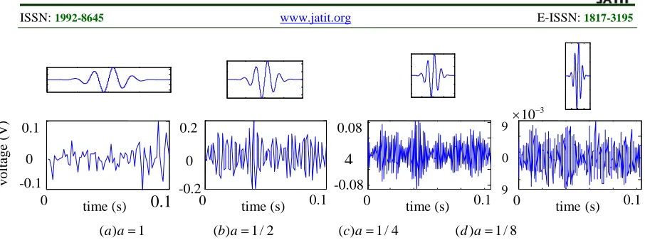
the following conclusion is: the principle of wavelet transform from low frequency to high frequency is consistent with the thought of recognizing essence of things from collectivity to part, and from macroscopy to microcosm. Figure 3 shows the four-level wavelet decomposition results of time sequence signals decomposed by Db4 orthogonal wavelet. The upper four figures are Db4 orthogonal wavelets of different scales, while the lower four figures are high frequency coefficients of wavelet decomposition. Since the process of recognizing things through fractal is to measure signals with a length ruler of different scales, and studying the essential characteristics of things by measurement results, while wavelet transform is with a wavelet ruler of different scales, fractal and wavelet transform have similar process by comparing figure 1 with figure 3.

Chirplet transform is the extension of short-time

Fourier transforms (STFTs) and wavelet

transforms[9]. It has time-frequency (TF) locality as wavelet transform, and its time-frequency window is more flexible than wavelet transform. Wavelet is a signal wave obtained through modulating

harmonic oscillations with a short fundamental wave, while chirplet is achieved by modulating linear frequency modulation (FM) oscillations with a short fundamental wave. Chirplet transform includes not only translation in time and frequency, and dilation in frequency, but also dilation and rotation of rectangular mesh along oblique direction, through which the time-frequency features of non-stationary signals are presented efficiently.

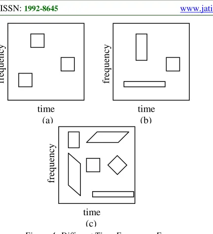
Affine time-frequency transform of short Fourier, wavelet and chirplet[9] are shown in figure 4. In figure 4(a), time-frequency mesh is just translated in time and frequency, but complex change is shown in figure 4(b), which includes dilations in time and frequency besides aforementioned changes, in other words, short Fourier transform analyzes mesh with invariable time-frequency in shape and size, but wavelet transform, whose bandwidth is proportional to frequency, analyzes mesh with the time-frequency,. According to time-frequency uncertainty principle, the area of mesh is constant. Therefore, short Fourier transform is suitable for non-stationary signals with constant bandwidth, but wavelet transform for non-stationary signals with changeless proportional bandwidth. However, signals often approximately equal to constant proportional bandwidth in practical application, whose analyses need more complex time-frequency mesh than rectangle. Thus chirplet transform appears, with dilations and rotations of rectangular mesh in oblique direction considered, as shown in figure 4(c).

[image:3.612.76.529.69.238.2]

( )a a=1

( )b a=1 / 2

( )c a=1 / 4

( )d a=1 / 8

Figure 3: Wavelet Decomposition Of Time Sequence Signals 0.1

-0.1 0

vol

ta

ge

(

V

)

0.1

0 _{time (s)}

0.2

-0.2 0

0.1

0 _{time (s)}

-0.08 0.08

4

0.1

0 _{time (s)} 9

9

0

0.1

0 _time_(s)

3

10−

(4)

[image:4.612.83.539.68.518.2] [image:4.612.315.531.71.536.2] [image:4.612.90.306.73.310.2]

358

Figure 5 shows five different affine

transformations, and table 1 shows the operators corresponding to the coordinate axes of the chirplet transform parameter space[9].

The wavelet provides a tiling of the TF plane with tiles that are lined up with the time and frequency axes, whereas the chirplet construct a more general tiling of the TF plane because the tiles may rotate or shear. As a matter of fact, wavelet can be regarded as chirplet with zero FM slope. Hence, it is easy to understand that chirplet transform is

extension of wavelet

.

It is readily discernible that

fourier transform and wavelet transform are special cases of chirplet transform[9]. Consequently, chirplet transform can provide more characteristics of signals than wavelet transform.

Based on this idea, a new dimension is proposed

in this paper, namely chirplet-fractal dimension, by describing the results of chirplet transform[10] with the concept of fractal dimension, that is, the fractal characteristics of signals is expressed by chirplet-fractal dimensions.

Chirplet-fractal dimension is defined as follows:

1) Decompose signals with orthogonal chirplet transform, then high frequency coefficients are results of measuring signals with chirplet ruler. And note the coefficients with different scales as:

{

Dj k, k=1, 2,Mj

}

(6)

where

j

is the level of decomposition, and Mj is

the sample length of high frequency sequence in chirplet transform.

2) Take the sum of the absolute values of modified coefficients as a measurement of decomposition result obtained by chirplet transform, note it as:

2

, 1 j

M

j j k

k

S D

=

∑

(7)

fr

eque

nc

y

time (a)

fr

eque

nc

y

time (b)

fr

eque

nc

y

time (c)

Figure 4: Different Time-Frequency Form

0.5

-0.5

fr

eque

nc

y

Shear in frequency Shear in time

Translation in frequency Translation in time

0

time(s) 100

0.5

-0.5

fr

eque

nc

y

0

time(s) 100 0

time(s) 100

0

time(s) 100 0

time(s) 100

0.5

-0.5

fr

eque

nc

y

0.5

--0.5

-0.5

fr

eque

nc

y

0

time(s) 100 0

time(s) 100

0.5

-0.5

fre

q

u

en

cy

0.5

-0.5

fr

eque

nc

y

Dilation in time _{Dilation in frequency}

Original function

0.5

-0.5

F

req

u

en

cy

(5)

359

Table 1 Five Operators Corresponding To Chirplet Transform

1-parameter notation Composite notation Time domain g(t)

Time translation ( )

c

tg t

→

→ =Mtc,0,0,0,0g t( ) g(t-tc)

Frequency

translation ↑↑tcg t( ) =M0,fc,0,0,0g t( )

2 c _{( )}

j f t

e π g t

Time dilation

/Frequency dilation ↔↔ag t( ) =M0,0, ,0,0a g t( ) e

-a/2

g[e-a(t-a)]

Time shear ( )

pg t

 =M0,0,0, ,0p g t( )

2 1 1/ 2

(₋_jp)− _ejπpt _∗_{g t}( ) Frequency shear ↓↑_qg t( ) =M_0,0,0,0,qg t( )

2 2

2 _{( )} q j t

e π g t

3) Plot the curve of lnj~ lnS_j , then get

Richardson plot in a similar way as box dimension, and divide the curve into three regions A, B and C in terms of different slopes, and regard region B as the scale-free region. Suppose the start point

and the end point of this region are

j

₁ and

j

₂,

respectively, then ln j~ lnS_j satisfies linear

regress model:

1 2

lnS_j= −D_Clnj b+ , j ≤ ≤j j (8)

The slope D_C is defined as chirplet-fractal

dimension of discrete sequence, and can be gotten through least square method:

(

)

2 1

2 2

2 1

( 1) ln ln ln ln

( 1) ln ln

j j

C

j j j S j S

D

j j j j

− + −

= −

− + −

∑

∑ ∑

∑

(9)

where j₁≤ ≤j j₂.

3. TESTS AND RESULTS

3.1Test Model

The chirplet-fractal dimension of LC on HV insulators is gotten from the method proposed in this paper. And LC is gotten from the following artificial test of contaminated insulator flashover: the test is under the condition of clean fog, constant voltage and contaminating beforehand with solid pollution method. The fog room is

1.8m× 1.8m× 2.0m in size, the rated capacity,

rated current and rated voltage of the variable

transformer are 125/250 kVA , 312.5/0.5 A and

0.4/250kV , respectively. The tested insulator is

XP-70. Among 7 pieces of insulator string in

63 kV to simulate 110 kV transmission lines,

NSDD is 2.0_{mg cm}_/ 2_{, ESDD are 0.10}_{mg cm}_/ 2_,

0.15_{mg cm}_/ 2_{, and 0.20}_{mg cm}_/ 2_{, respectively.}

3.2Results

The chirplet-fractal dimension of denoised LC is calculated through the method mentioned above. Figure 6 to figure 11 are LC curves of the artificial test and the corresponding chirplet-fractal dimensions, and their ESDD are 0.10, 0.15 and

0.20 2

/

mg cm , respectively.

The chirplet-fractal dimensions of LC decreases along with the increasing of the LC amplitude. In initial stage, because pollution layer is being humidified in low humidity, the impact of LC is very small with sporadic spark and glow discharge, and the corresponding chirplet-fractal dimension changes hardly. Little arcs begin to discharge along with sufficiently humidified pollution layer, which leads to large impacts of LC. But owing to a few distinguish among intensities of little arcs and multiple little arcs existing at one time, the impacts of arcs discharge counteract each other, which results in some fluctuation of LC[11], and the corresponding chirplet-fractal dimension increases evenly. And then a big arc occurs and develops to the primary arc, meanwhile, LC fluctuates obviously[12]. While the primary arc runs through the whole insulator string and the flashover was brought on, LC presents a very large impact, shown as the final impact current close to 0.3A in Figures 6, 8, and 10, and the chirplet-fractal dimension concusses acutely. At the moment of flashover, the chirplet-fractal dimension decreases heavily, shown as the time of 19 in Figure7, time of 18 and 20 in Figure8, and time of 14 and 20 in Figure11.

(6)

360 Figure 6: Leakage Current (ESDD=0.10)

0 2 4 6 8 10 12 14 16 18 20 22 24 0.000

0.025 0.050 0.075 0.100 0.125 0.150 0.175 0.200 0.225 0.250

chi

rpl

et

-f

rac

tal

di

m

ens

ion

index

[image:6.612.91.528.78.488.2]

Figure 7: Chirplet-Fractal Dimension Of Figure 6

Figure 8: Leakage Current (ESDD=0.15)

0 2 4 6 8 10 12 14 16 18 20 22

0.000 0.025 0.050 0.075 0.100 0.125 0.150 0.175 0.200 0.225 0.250

chi

rpl

et

-f

rac

tal

di

m

ens

ion

[image:6.612.111.282.391.679.2]

index

Figure 10: Leakage Current (ESDD=0.20)

0 2 4 6 8 10 12 14 16 18 20 22 0.000

0.025 0.050 0.075 0.100 0.125 0.150 0.175 0.200 0.225 0.250

chi

rpl

et

-f

rac

tal

di

m

ens

ion

index

final stage. Especially, the chirplet-fractal dimension decreases heavily when LC concusses acutely. This shows that the chirplet-fractal dimension describes the information of arcs discharge in LC efficiently. Therefore, taking chirplet-fractal dimensions of LC as the eigenvalue can reflect the change law of LC during the flashover, and the supervision of LC can be realized exactly through the change of chirplet-fractal dimension.

4. CONCLUSION

A new idea called chirplet-fractal dimension, using chirplet as the ruler to define fractal dimension, is proposed in this paper, and the algorithm is described too.

[image:6.612.111.279.527.669.2]

(7)

361

0 2 4 6 8 10 12 14 16 18 20 22

-0.025 0.000 0.025 0.050 0.075 0.100 0.125 0.150 0.175 0.200 0.225 0.250

chi

rpl

et

-f

rac

tal

di

m

ens

ion

index ESDD=0.15 ESDD=0.20 ESDD=0.10

Figure 12: Chirplet-Fractal Dimensions Of LC

REFERENCES:

[1] Ramirez, Isaias, Hernández, Ramiro, Montoya,

Gerardo, “Measurement of leakage current for monitoring the performance of outdoor

insulators in polluted environments”, IEEE

Electrical Insulation Magazine, Vol.28, No.4, 2012, pp. 29–34.

[2] Douar, M. A., Mekhaldi, A., Bouzidi, M. C.,

“Flashover process and frequency analysis of the leakage current on insulator model under

non-uniform pollution conditions”, IEEE

Transactions on Dielectrics and Electrical Insulation, Vol.17, No.4, 2010, pp. 1284-1297.

[3] Chandrasekar, S., Kalaivanan, C., Cavallini,

Andrea, Montanari, Gian, “Investigations on

leakage current and phase angle characteristics of porcelain and polymeric insulator under

contaminated conditions”, IEEE Transactions

on Dielectrics and Electrical Insulation, Vol.16, No.2, 2009, pp. 574-583.

[4] Boudissa, Rabah, Djafri, Saâdi, Haddad,

A., Belaicha, R. Bearsch, R., “Effect of

insulator shape on surface discharges and

flashover under polluted conditions”, IEEE

Transactions on Dielectrics and Electrical Insulation, Vol.12, No.3, 2005, pp. 429-437.

[5] Y. Mizuno, K. Naito, W. Naganawa, “A study

on probabilistic assessment of contamination

flashover of high voltage insulators”, IEEE

Transaction on Power Delivery, Vol.10, No.3, 1995, pp. 1378-1383.

[6] Benoit Mandelbrot, “How long is the coast of

Britain? Statistical self-similarity and fractional

dimension”, Science, Vol.156, No.3775, 1967,

pp. 636-638.

[7] Tang, Dongming, Marangoni, Alejandro G.,

“Computer simulation of fractal dimensions of

fat crystal networks”, Journal of the American

Oil Chemists' Society, Vol.83, No.4, 2006, pp. 309-314.

[8] Delgado Prieto, Miguel, Garcia Espinosa,

Antonio, Riba Ruiz, Jordi-Roger, Urresty, Julio

César, Ortega, Juan Antonio, “Feature

extraction of demagnetization faults in permanent-magnet synchronous motors based

on box-counting fractal dimension”, IEEE

Transactions on Industrial Electronics, Vol.58, No.5, 2011, pp. 1594-1605.

[9] Steve Mann, Simon Haykin, “The chirplet

transform: physical considerations”, IEEE

Transactions on Signal Processing, Vol. 43, No.11, 1995, pp. 2745-2761.

[10]Yufeng Lu, Ramazan Demirli, Guilherme

Cardoso, Jafar Sanii, “A successive parameter estimation algorithm for chirplet signal

decomposition”, IEEE Transactions on

Ultrasonics, Ferroelectrics, and Frequency control, Vol.53, No.11, 2006, pp. 2121-2131.

[11]Chrzan, Krystian Leonard, Moro, Federico,

“Flashover of contaminated nonceramic

outdoor insulators in a wet atmosphere”, IEEE

Transactions on Power Delivery, Vol.22, No.1, 2007, pp. 466-471.

[12]Dhahbi-Megriche, N. Beroual, A., “Dynamic

model of discharge propagation on polluted

surfaces under impulse voltages”, IEE