Bayesian Model Selection and
Forecasting in Noncausal Autoregressive
Models
Lanne, Markku and Luoma, Arto and Luoto, Jani
University of Helsinki, HECER, University of Tampere
September 2009
Online at
https://mpra.ub.uni-muenchen.de/23646/
Discussion Papers
Bayesian Model Selection and Forecasting in
Noncausal Autoregressive Models
Markku Lanne
University of Helsinki and HECER
Arto Luoma
University of Tampere
and
Jani Luoto
University of Helsinki and HECER
Discussion Paper No. 273 September 2009
ISSN 1795-0562
HECER – Helsinki Center of Economic Research, P.O. Box 17 (Arkadiankatu 7), FI-00014 University of Helsinki, FINLAND, Tel +358-9-191-28780, Fax +358-9-191-28781,
Discussion Paper No. 273
Bayesian Model Selection and Forecasting in
Noncausal Autoregressive Models*
Abstract
In this paper, we propose a Bayesian estimation and prediction procedure for noncausal autoregressive (AR) models. Specifically, we derive the joint posterior density of the past and future errors and the parameters, which gives posterior predictive densities as a by-product. We show that the posterior model probability provides a convenient model selection criterion and yields information on the probabilities of the alternative causal and noncausal specifications. This is particularly useful in assessing economic theories that imply either causal or purely noncausal dynamics. As an empirical application, we consider U.S. inflation dynamics. A purely noncausal AR model gets the strongest support, but there is also substantial evidence in favor of other noncausal AR models allowing for dependence on past inflation. Thus, although U.S. inflation dynamics seem to be dominated by expectations, the backward-looking component is not completely missing. Finally, the noncausal specifications seem to yield inflation forecasts which are superior to those from alternative models especially at longer forecast horizons.
JEL Classification: C11, C32, C52, E31
Keywords: Noncausality, Autoregression, Bayesian model selection, Forecasting.
Markku Lanne
Department of Economics, P.O. Box 17 (Arkadiankatu 7) FI-00014 University of Helsinki FINLAND
Arto Luoma
Department of Mathematics and Statistics
FI-33014 University of Tampere
FINLAND
Jani Luoto
Department of Economics, P.O. Box 17 (Arkadiankatu 7) FI-00014 University of Helsinki FINLAND
1. Introduction
Univariate autoregressive (AR) models have several uses in analyzing economic time series.
However, it is the causal AR model that has almost exclusively been employed in econometrics
although noncausal models have also to some extent been considered in statistics in general. The
main difference between the causal and noncausal AR models is that the latter allow for dependence
on future as well as past values of the variable in question, whereas the former force the variable to
depend only on its past. In the areas of economics where AR models are employed, expectations
typically play a central role, and, therefore, extensions to noncausal models are likely to open up
new possibilities, because they make explicit the dependence on future errors and values of the
variable.
The literature on noncausal AR models is not voluminous, and so far very few economic
applications exist. Apart from Lanne and Saikkonen (2008), who found strong support for a
noncausal AR specification for the U.S. inflation, previous studies on noncausal AR and related
models in statistics only contain brief illustrations of the methods using economic data, but no
serious applications.1 Lanne and Saikkonen (2008) recently introduced a new formulation of the
noncausal AR model that has a number of statistical advantages in addition to allowing for a
convenient interpretation in terms of expectations, likely to be useful in economic applications.
They also derived an approximate maximum likelihood estimator of this formulation and the related
asymptotic distribution theory. Because causality and noncausality are not distinguishable under
Gaussian errors, Lanne and Saikkonen (2008) suggested using Student's t-distribution, which seems
appropriate in view of the fact that in economic applications residuals often turn out to deviate from
normality in the direction of excess kurtosis. However, within their formulation of the model that
we also consider in this paper, various alternative distributional assumptions can also be
entertained.
Allowing for noncausality complicates model selection. Even if an economic variable can be
assumed to be characterized as an AR process, causality or noncausality cannot be determined on
the basis of its autocorrelation structure because there are multiple causal and noncausal models of
1
Breidt et al. (2001) fit a noncausal first-order AR model to a daily time series of the trading volume of Microsoft stock
and the closely related all-pass model to the New Zealand/U.S. exchange rate. Huang and Pawitan (2000) applied a
the same order producing identical autocorrelation functions. As pointed out above, with Gaussian
errors, alternative causal and noncausal models of the same order also produce the same value of
the likelihood function. Therefore, a non-Gaussian error distribution must be assumed, but even in
that case model selection cannot be based on testing in a straightforward way because the
alternative specifications are not nested. Following Breidt et al. (1991), Lanne and Saikkonen
(2008) proposed a model selection procedure based on the maximum value of the likelihood
function over a number of different model specifications of the same order and subsequent
diagnostic checks for the adequacy of the model proposed by this criterion. In this paper, we
consider the Bayesian analysis of noncausal AR models. We adopt the formulation of Lanne and
Saikkonen (2008) and concentrate on model selection, since the nonnestedness of the models to be
compared poses no particular problem in Bayesian analysis. Specifically, we use the posterior
model probability of a particular specification to assess the degree of support in the data for that
specification. The posterior model probabilities are based on an exact likelihood function where the
past and future errors are considered unknown parameters. Thus the inference is not conditional on
initial values. This is convenient in small samples, since in the conditional approach the number of
starting values rapidly increases as a function of the orders of the autoregressive polynomials.
Our simulation experiments indicate that the proposed Bayesian model selection criterion works
well in discriminating between causal and noncausal AR models. In particular, the expected
posterior probabilities in favor of noncausal processes are high even under a relatively low degree
of noncausality. On the other hand, when the true data generating process is causal, our model
selection criterion selects the noncausal model markedly less frequently than the procedure of
Breidt et al. (1991) and Lanne and Saikkonen (2008). This indicates that the probability of falsely
selecting the noncausal process is lower with our criterion.
We consider an empirical application to the same U.S. inflation series that Lanne and Saikkonen
(2008) used, and in accordance with their results, we find support for the purely noncausal AR
model, where current inflation only depends on expected future inflation. The posterior medians of
the purely noncausal AR model are also very close to those obtained by Lanne and Saikkonen
(2008). Taken at face value, this finding indicates that the observed persistence in inflation is
caused by the predictability of inflation instead of agents' relying on past inflation in forming
expectations. However, even though the purely noncausal model turns out to be the likeliest by far,
the probabilities of the other noncausal specifications, with dependence also on past inflation, are
which goes contrary to typical New Keynesian models with forward-looking dynamics, but accords
with much of the recent empirical literature. In contrast to that literature relying on causal AR
models, though, we find expectations of future inflation to be the most important factor causing
persistence. From the viewpoint of economics, this kind of availability of a measure of the
likelihood of the purely noncausal model vis-à-vis the alternative AR models is probably the
greatest value-added of Bayesian over classical analysis.
For optimal prediction of a noncausal process, knowledge of future errors is required. Because our
approach treats these as unknown parameters, it has the advantage of providing a straightforward
way to compute forecasts. Moreover, in addition to employing a single model to produce forecasts,
Bayesian model averaging is readily available. According to our out-of-sample forecasting
exercise, the forecasts of inflation based on noncausal AR models turned out, in general, to be
superior to those based on causal models, especially at longer forecast horizons. In most cases, the
model suggested by our criterion produce the most accurate forecasts, only in the most recent
subsample period did Bayesian model averaging produce the most accurate results.
The plan of the paper is as follows. In Section 2, the noncausal AR model is presented and the
likelihood function is derived. In Section 3, the choice of prior distributions is discussed. Section 4
shows how posterior analysis can be conducted. In Section 5, we describe the principles of model
selection and present the results of the related simulation study. Section 6 presents the results of the
empirical application to the U.S. inflation. Finally, Section 7 concludes.
2. The model
Consider a stochastic process, yt (t = 0, ±1, ±2,…), generated by
L
L yt t 1
, (1)
where
L L1sLs1 1
1 ,
L 11LrLr, εt is a sequence of i.i.d. randomvariables with zero mean and variance σ2 and L is the lag operator. The autoregressive process
defined in equation (1) is noncausal if j ≠ 0 for some j{1,…,s} and it is referred to as purely
that has the conventional causal AR model as a special case when s = 0 (see Lanne and Saikkonen,
2008, and the references therein).
In equation (1), we assume that the roots of the equation
z 0 lie outside the unit circle, andhence the process
L1 yt ut has the following moving average representation,
0
j
j t j t
u , (2)
where α0 = 1 and the coefficients αj decay to zero at a geometric rate as j → ∞. Similarly, we
assume that the roots of
z 0 lie outside the unit circle, implying that the process
L yt vthas the following moving average representation, showing dependence on future errors,
0
j
j t j t
v , (3)
where β0 = 1 and the coefficients βj decay to zero at a geometric rate as j→∞. The process yt itself
has the two-sided moving average representation
j
j t j t
y , (4)
where ψj is the coefficient of zj in the Laurent series expansion of
z
z
zdef
1 1 1
. Thus, yt is
a stationary and ergodic process with finite second moments.
Lanne and Saikkonen (2008) studied the maximum likelihood (ML) estimation of the noncausal
autoregressive model specified in equation (1). In particular, they derived an approximate likelihood
function in which the first r and last s observations are treated as fixed initial values. In this paper,
an alternative approach is suggested, where also these observations and, hence, past and future
errors are explicitly modeled by treating them as unobserved missing observations or unknown
parameters. This is likely to improve estimation and is particularly useful in model comparison and
optimal prediction of a noncausal process, knowledge of future errors is required, and, therefore,
our approach has the advantage of allowing for straightforward way of computing forecasts.
For the Bayesian analysis of the noncausal AR model, we need to derive the joint probability of the
observations conditional on the parameters, i.e., the likelihood function, and specify the prior
distributions of the parameters. Let us start with the likelihood function and defer the priors to
Section 3. A truncated joint density function of the data y = (y1, y2,…,yT) and the past and future
errors conditional on the vector of parametersθ= (1,,r, 1,,s, σ, ν')', can be expressed as
ε ε
y
ε ε
ε
y
ε , , p p p , ,
p , (5)
where ε- = (ε-M,…,ε-1, ε0), ε+ = (εT+1, εT+2,…,εT+M), ν is an additional parameter vector consisting of
the parameters that determine the shape of the error distribution, and the truncation parameter M is a
positive integer, chosen to be large enough for a sufficiently good approximation of the joint density
of the data, the last term on the right-hand side of equation (5). The likelihood function can be
obtained by integrating out the past and future errors from the joint density (5),
ε ε y ε ε ε ε
y p p p d d
p , , . (6)
In a general case, this integral cannot be computed analytically. However, an applicable numerical
solution can be obtained once the distribution of the errors εt has been chosen. In the following, we
shall describe how such a solution can be obtained.
We start by deriving the joint density function of the errors ε = (ε-, u1,…,ur, εr+1,…,εT-s, vT-s+1,…,vT,
ε+
) and then obtain p
ε,y,ε
by means of the change of variables theorem. The ultimate goal is to express the known joint density of errors ε1,…,εT as a function of the given data y. Because theerrors ε-, u1,…,ur, vT-s+1,…,vT, and ε+ are independent of εr+1,…,εT-s, as can be seen from equations
(2) and (3), the joint density function of ε has the expression
ε
εε , , , 1, , ,
1
1 T s T
s T
r t
t
r f pv v
u u p
T M
T t t T s T s T r t t r M t
t pu u f pv v f
f 1 1 1 1 0 , , , , , ,
ε ε , (7)
where the error distribution is assumed to be non-Gaussian with density fσ(x) = σ-1f(σ-1x, ν). As in Lanne and Saikkonen (2008), the density function fσ(·) satisfies the regularity conditions of Andrews et al. (2006) which, among other things, require that fσ(·) is twice continuously differentiable with respect to x and ν, non-Gaussian, and positive for all real numbers x and all
permissible values of the ν.
Now, by change of variables from (u1,…,ur, εr+1,…,εT-s, vT-s+1,…,vT) to y, equation (5) can be
expressed as
T s
r t t r M t
t p L y L y f L L y
f p 1 1 1 1 1 0 , , , ,
,y ε ε
ε
p
L y
L y
f
A M T T t t T s T
11, , ,
ε , (8)
where |A| is the Jacobian determinant of the linear transformation given by equations
1 11 L y
u ,
21
2 L y
u ,…,uTs
L1 yTs, vTs1
L yTs1,…,vT
L yT (see Lanne and Saikkonen,2008, for a detailed derivation of the joint density of y). As a final step, we write
L1 y1, , L1 yr ε,
p and p
L yTs1,,
L yT ε,
in terms of the errors εt.Recalling that
L ut
L1 vt t and noticing that the Jacobian determinants of thetransformations from p
u1,,urε,
to p
1,,rε,
, and from p
vTs1,,vT ε,
to
Ts1, ,Tε,
p are unity, equation (8) can be written as
T s
r t t r t t M t
t f L u f L L y
f p 1 1 1 0 , ,
,y ε ε
ε
f
L v
f
A M T T t t T s T t t
1 1 1 ,
where u1
L1 y1,…,ur
L1 yr and vTs1
L yTs1,…,vT
L yT, that is, u1,…,ur andvT–s +1,…,vT are calculated from the data.
Evaluating the right-hand side of equation (9) requires knowledge of u1-r,…,u0 and vT+1,…,vT+s,
which cannot be computed directly from the data, but they can be obtained, for example, by the
following simple recursive calculations. From equation (1) we have
s M T s M
T M T M
T v v
v 1 1 ,
1 1
1
1
M T M T M s T M s
T v v
v ,
1 2
1 1
1
T T s T s
T v v
v , (10)
and plugging in the simulated values of εT+1,...,εT+M and setting vT+M+1,…,vT+M+s at their expected
value 0, we get vT1,..., vTM. Similarly,
r M r M
M
M u u
u 1 1 ,
1 1
1
1
M M u M ru M r
u ,
r ru u
u0 0 1 1 , (11)
where u-M-1,…,u-M-r, in turn, are set at zero.
In what follows, we assume that the elements of ε- and ε+ are unobserved variables, whose posterior
densities are obtained by simulation methods along with the unknown parameters. This, of course
facilitates a numerical solution for the integral (6). Furthermore, as pointed out above, explicit
incorporation of the past and future errors into the analysis allows for computing optimal forecasts
from a noncausal AR model in a straightforward manner. Specifically, the posterior densities of
vT+1, vT+2,…,vT+M may be simulated using equation (10) and the posterior distributions of θ and εT+1,
εT+2,…, εT+M. Then the predictive densities of the future observables yt+1,…,yt+h can be calculated
using the recursive formulayth 1yth1rythr vth. The means or medians of these
predictive distributions can be used as point forecasts. Notice also that when the process is purely
3. Priors
In addition to the likelihood function derived in Section 2, Bayesian analysis requires the
specification of prior distributions of the parameters of interest, 1,,r, 1,,s, σ and ν. We
use proper priors for these parameters because when improper priors, i.e. priors that are not well
defined density functions, are used for parameters occurring in one model but not the other,
posterior odds ratios are not identified (see O'Hagan, 1995). This is, of course, the case when
autoregressive models, with the unknown orders of the autoregressive polynomial operators, are
compared.
For the parameters 1,,r and 1,,s we adopt a multivariate Student prior,
s
r
1,, , 1,, ~ ts+r(μ,1,P,ν0), with mean vector μ and covariance matrix P–1/(ν0–2) (see
Bauwens, Lubrano, and Richard, 1999). This prior corresponds to the familiar conjugate
normal-inverted gamma prior for linear regression models when the scale parameter of the normal-inverted gamma
distribution is set at unity. We assume that μ is a zero vector, P = k I, where I is an identity matrix, k
is a scalar, and ν0 equals 3. We set k at unity, indicating an identity prior covariance matrix because
when posterior odds are used in model comparison, a value of k substantially less than 1
(uninformative prior) typically penalizes long lags and leads, whereas a value of k greater than 1
(informative prior) favors long lags and leads. Alternatively, we could use, for example, a
multivariate normal prior with an identity covariance matrix.
In order to study how our multivariate Student prior affects the posterior, a small simulation
experiment is carried out. Specifically, we compare the posterior modes based on the Student and
normal priors and the ML estimator. The data are generated as follows. First, starting with u1 =…=
ur = 0, a series from the causal model
L ut t (t = r+1,…,T) is generated. Then yt is computedrecursively from
L1 yt ut for t = T – s,…,1 by setting yT-s+1 =…= yT = 0.2 We follow Lanneand Saikkonen (2008) and assume from now on that the error term εt has Student’s t-distribution
with ν > 2 degrees of freedom and variance σ2. We set ν at 3 and σ2 at 1 and consider three different
combinations of parameters values, (1, 1) = {(0.1,0.7), (0.7,0.1), (0.7,0.7)}. In the first case, the
data generating process (DGP) is close to purely noncausal, in the second case it is close to causal,
and in the third case the roots of the lag polynomial are equal. A gamma prior with mean and
2
variance set at unity is adopted for σ and an exponential prior forν – 2, where the mean of ν is set at
3 (these priors are explained in detail below). The results are based on a series of 150 observations
(the time series used in our empirical application in Section 6 consist of 148 observations) and
1,000 replications. Table 1 presents the means and standard deviations of the posterior mode
estimates of 1and 1 based on both the Student and normal priors as well as the means and
standard deviations of the ML estimators obtained using the approximate likelihood function of
Lanne and Saikkonen (2008). As one would expect, the differences between the ML and posterior
results are minor. Thus, in this sense, both of these priors have only negligible influence on the
posterior inference. The results based on several different DGPs (not reported) are also similar, but
it seems that the posterior density is affected more strongly by the multivariate normal prior than by
the Student prior (with ν0 = 3) when the number of lags (and leads) increases. Therefore, we
recommend using the Student prior.
In order to seek for a suitable prior for σ, we estimated several posterior distributions of θ using
different priors for σ, the full likelihood function (9) and the priors (for other parameters) and the
artificial data used above. Our estimation results (not reported) indicate that the posterior
distribution of σ has a long right tail. Therefore, we recommend using a tight prior on σ to facilitate
numerical maximization. A gamma prior with mean and variance set at unity seems to work well in
our experiments and it is the prior adopted in our simulation study in section 5 and empirical
application in Section 6.
Finally, as shown by Bauwens and Lubrano (1998), sufficient prior information is needed on the
degrees of freedom parameter ν in Student’s t distribution to force the posterior, in order to be
integrable, to tend to zero quickly enough at the tail. We will follow Geweke (1993) in using an
exponential density. For computational reasons we give an exponential prior for ν – 2 (instead of ν)
and, in our simulation study, set the prior mean of ν at 3, which implies a tight prior variance, unity.
In the empirical application we give more weight to the data and set the prior mean of ν at 7.
4. Posterior analysis
With the likelihood function derived in Section 2 and the prior distributions specified in Section 3,
we are able to compute the posterior distribution of the parameters θ and the past and future
product of the marginal prior densities of the previous section and the joint density of the data,
respectively. The joint posterior density of ε-, ε+ and θ can then be expressed as
) ( , , , , y ε y ε y ε ε p p pp
d d d p p p p ε ε ε y ε ε y ε , , , , . (13)
It is obvious that a closed form solution exists for neither the marginal likelihood p(y) nor the
posterior moments of the parameters, and numerical methods are required. Because none of the full
conditionals of the density (13) are in the form of any standard probability density function (p.d.f.),
we apply the Metropolis-Hastings algorithm.
We first apply the logarithmic transformations for the parameters σ and ν to obtain approximate
normality of their marginal posteriors, which makes the posterior simulations markedly more
efficient. Let η = (1,,r,1,,s, ln σ, ln (ν – 2))' denote the vector of the transformed
parameters. As starting values we use a zero vector for ε- and ε+ and the posterior mode for η.3
In the ith iteration (i = 1,…,N) we draw a candidate η* from the normal proposal density and accept
it with probability
1 1 1 1 1 1 1 1 1 1 * * 1 * 1 * , , , , , 1 min i i i i i i i i i i i i p p p p p p p p ε ε y ε ε ε ε y ε ε . (14)
3
To get a convenient proposal density for θ, we minimize the negative of the logarithm of the posterior density
numerically (using the approximate likelihood function of Lanne and Saikkonen, 2008) to obtain the posterior mode of
the transformed parameter vector η and evaluate the Hessian matrix at the minimum. We then compute the inverse of
the Hessian to approximate the posterior covariance matrix of η and scale it by the factor 2.42/(s+r+2) to obtain the
optimal covariance matrix Σ for the multivariate normal proposal distribution fN(η|η(i-1), Σ) (i = 1,…,N). Notice that the
greater is the number of iterations N, the more precise are the posterior estimates. In some cases the covariance matrix
estimate based on the local behavior of the posterior at its highest peak gives too optimistic a view of precision and thus
fails to yield an efficient covariance matrix for the normal proposal distribution. In these cases, starting with the inverse
of the Hessian in the proposal distribution we first simulate a certain number of posterior draws, use them to estimate
Cov(θ|y, ε-, ε+), and then set Σ = 2.42Cov(θ|y, ε-, ε+)/(r+s+2) (see e.g. Gelman et al., 2004). This is repeated until a
If η* is not accepted, we set η(i) at its current value. The one-to-one mapping between η and θ is
used.4
We continue by drawing a candidate ε-* using p(ε-|θ(i)) = fσ(ε-M|θ(i))···fσ(ε0|θ(i)) as the candidate
generating density, and hence by the definition of the acceptance probability of the
Metropolis-Hastings algorithm, the acceptance probability of this step simplifies to
r t i i t r t it f L u
u L f 1 1 1 * , , , 1
min
ε ε . (15)
We set ε i ε* with probability α and ε i ε i1 with probability 1 – α. Similarly, we take a
candidate draw ε+* from density p(ε+|θ(i)) = fσ(εT+1|θ(i))···fσ(εT+M|θ(i)) and calculate an acceptance
probability
t i iT s T t i t T s T t v L f v L
f
min 1, , 1 1,
1 *
1
1
ε
ε . (16)
Again we set ε i ε* with probability α and ε i ε i1 with probability 1 – α.
When several alternative models are estimated by the method discussed above, typically model
comparison is of interest, and it can conveniently be based on the marginal likelihoods of the
alternative models. For each noncausal AR model specification, Mj (j = 1,...,J), the marginal
likelihood is simply the denominator of the joint posterior density (13),
d d d M p M p Mpy j j ε ,y,ε , j ε ε . (17)
This can be estimated from the simulated posterior sample using, for example, the reciprocal
importance estimator of Gelfand and Dey (1994), given by
4
Notice that by change of variable the prior of = ln (ν – 2) is given by p( ) = λexp{–λe + }, where -∞ < < ∞
11 , 1 ˆ
Gg jg j jg j
g j j M p M p f G M p y
y , (18)
where γj = (εj-, εj+, ηj) is the vector of all unobservable variables, p(y|γj,Mj) is the likelihood for
model Mj defined on region Γj, p(γj|Mj) is the corresponding prior density, f(γj) is any p.d.f. with
support contained in Γj and
G g g j 1
is a sample of size G from the estimated joint posterior
distribution. We decided to use this method because it is based on straightforward calculations and
does not require the evaluation of the posterior density p(γj|y,Mj), which may be difficult in our
case. It also seems to work well in practice as long as the truncation parameter M is not too large.
For large M, the dimensionality of the parameter space may become too high, making the method
inaccurate.
The asymptotic theory behind the method of Gelfand and Dey (1994) implies that
f(γj)/[p(γj|Mj)p(y|γj,Mj)] must be bounded from above (see e.g. Koop, 2003). To verify that this
quantity is finite for all possible values of γj, we follow Geweke (1999)and let f(γj) be a truncated
multivariate normal density
m j
j j
j j j
j j
j p
f
ˆ ˆ ˆ 1
2 1 exp ˆ
2
1 1/2 1
2 /
'
, (19)
where ˆ and j ˆ are estimates of the mean and covariance matrix of the posterior density, j
respectively. The indicator function 1(•) takes the value 1 when jj, where
j j j j j j p j
j m 2 1 1 ˆ ˆ ˆ : '
, (20)
j p m2 1
is the (1–p)th percentile of the Chi-square distribution with mj degrees of freedom, and mj
5. Model comparison
So far, we have assumed the noncausal AR model specification known, which, of course, is
virtually never the case. Instead, the orders r and s of the polynomials
L and
L1 , respectively, must in practice be determined by the data. The nonnestedness of the alternativeAR(r,s) models complicates classical model selection, but poses no particular problems in Bayesian
analysis.
Given the marginal likelihoods p(y|Mj) of each of the J models Mj (j = 1,…,J) discussed in Section
4, model selection can be based on the posterior model probabilities. By assuming that our set of
models is exhaustive, we have from Bayes’ theorem that
J
i
i i
j j j
M p M p
M p M p M
p
1
y y
y , (21)
where J = (rmax+1)×(smax+1), and rmax and smax are maximum allowed lag and lead lengths,
respectively, and p(Mj) is the prior model probability assigned to model Mj. We assume that all the
models are equally likely a priori because as long as rmax and smax are reasonable, we have no reason
to assume otherwise. That is, we set p(Mj) = 1/J for all j, and seek the posterior model probabilities
p(Mj|y) of all the combinations of r = 0,…,rmax and s = 0,…,smax. The model with the greatest
posterior probability is selected. Lanne and Saikkonen (2008) suggest selecting the maximum lag
and lead lengths by first finding a Gaussian AR(rmax,0) model with rmax sufficiently great to
eliminate all serial correlation in the errors and then considering all AR(r,s) models with r + s =
rmax. Alternatively, information criteria could be employed.
To study the ability of Bayesian model selection in discriminating between causal and noncausal
specifications, we conducted a small simulation experiment. Throughout, the results are based on
1000 realizations of a series of 150 observations. To keep the number of simulations reasonable, we
restrict our attention to a simple case where rmax = smax = 1. Thus, the underlying data generating
process is
where the error terms εt are assumed to have the standardized Student’s t-distribution with 3 degrees
of freedom and variance unity. The data are generated from (22) with various positive values of 1
and 1 (given in Table 2 and 3). In order to reduce initialization effects, 100 observations at the
beginning and end of each realization are discarded. For each realization we estimate four different
models: a white noise model M1 (r = 0, s = 0), a causal model M2 (r = 1, s = 0), a purely noncausal
model M3 (r = 0, s = 1), and a noncausal model M4 (r = 1, s = 1).
The estimation is based on the posterior distribution (13), where the truncation parameter M is set at
20 and the joint prior density of Section 3 is used.5 Using demeaned data and the methods explained
in the previous section, the posterior model probabilities p(M4|y) and p(M3|y)+p(M4|y) are
calculated, and averaged over 1000 replications.6 The former quantity gives the mean posterior
probability of the true noncausal model (except when 1 = 0), and the latter the mean posterior
probability of a noncausal process, i.e., it can be interpreted as the overall probability of the
presence of noncausality. Following Marriot and Newbold (2000) we also consider the decision
rules p(M4|y) > 0.5 and p(M3|y)+p(M4|y) > 0.5, indicating that a model is selected if its posterior
model probability exceeds 50%. The means of the posterior model probabilities are presented in the
upper panels and the proportions of times when p(M4|y) > 0.5 or p(M3|y)+p(M4|y) > 0.5 are reported
in the lower panels of Tables 2 and 3, respectively.
As we would expect, the greater is the parameter1 the greater is the probability of a noncausal
processes. There is, however, one exception: When the true value of 1 is close to unity and 1 is
close to zero, the mean posterior probability of the noncausal process decreases sharply. Notice that
this is not a unit root issue. Rather, the noncausal and causal models are indistinguishable when 1
= 1 and 1 = 0 (or when 1 = 0 and 1 = 1). Therefore, as 1 approaches 1 under 1 ≈ 0, the
probability of incorrectly selecting the causal process increases sharply. Otherwise, the procedure
seems to perform fairly well in discriminating between causality and noncausality, selecting a
5
According to our simulation experiments (not reported) M = 20 is large enough to guarantee a sufficiently accurate
approximation to the joint density of observed data. 6
The number of simulation rounds N was set at 20000, and the first 2000 simulations in each chain were excluded as a
burn-in period. The convergence of the chains was checked using the standard convergence diagnostic of Geweke
(1992). To reduce the size of output files, every 9th draw is used in the calculation of marginal likelihoods, thus G =
noncausal process in over 85% of the replicates whenever the true value of 1 is greater than or
equal to 0.3.
Finally, we compare our Bayesian model selection procedure to that of Lanne and Saikkonen
(2008). They strongly recommend using diagnostic checks to confirm the adequacy of the model
suggested by the maximized likelihood criterion, but we ignore this step as it is difficult to
incorporate into the simulation experiment. For simplicity, we consider the case where the order of
the autoregressive polynomial operators is assumed to be known. In particular, we set r + s at 2 and
calculate the marginal likelihoods and the maximum values of the approximate log likelihood
function for the causal, purely noncausal and mixed models. We assume the same three parameter
combinations (1, 1) = {(0.1,0.7), (0.7,0.1), (0.7,0.7)} as in section 3. Again, the results (not
reported in detail) are based on 1000 realizations of a series of 150 observations where the error
terms εt are assumed to have the standardized Student’s t-distribution with 3 degrees of freedom and
variance unity. In general, the two procedures yield rather similar results although there are some
differences. For instance, compared to the classical procedure, the Bayesian criterion performs very
well when the process is clearly noncausal, selecting the true model in 76.7% and 98.4% of the
replicates when (1, 1) = (0.1, 0.7) and (1, 1) = (0.7, 0.7), respectively. The corresponding
classical figures are 67.9% and 96.5%. In contrast, when (1, 1) = (0.7, 0.1), the classical
procedure selects the true model in 70.1% of the replicates, while the Bayesian procedure only
reaches 59.1%. However, in this case, the true model is fairly close to the first-order causal
autoregressive model. Therefore, this result may reflect the tendency of the classical procedure to
select a noncausal process too frequently. Actually, when the data are generated from a purely
causal AR(2,0) process where1= 0.6 and 2= 0.2, the classical procedure selects the noncausal
model in 12.4% and the Bayesian procedure in 8.1% of the replicates.
6. Empirical application
Today, one of the most interesting macroeconomic phenomena is the U.S. inflation. Questions like
whether it is forward- or backward-looking or why it is so difficult to forecast it well have remained
without solid answers (see e.g. Rudd and Whelan, 2006, and Stock and Watson, 2007). Therefore,
the methods introduced in this paper are applied to the U.S. consumer price inflation. For the most
and lagged inflation should be interpreted as evidence of backward-looking inflation, but we also
consider forecasting inflation.
6.1. Posterior results
The specific inflation series we study is the annualized quarterly inflation computed from the
seasonally adjusted U.S. consumer price index (for all urban consumers). The series is published by
the Bureau of Labor Statistics. The sample period covers 148 observations from 1970:1 to 2006:4.
There is a substantial literature examining the behavior of this series (from different sample
periods). The series is found to be highly persistent, measured in terms of serial correlation, which
has been interpreted as evidence in favor of backward-looking behavior of price setters. However,
since causal and purely noncausal processes can have the same autocorrelation functions, the
backward-looking or forward-looking behavior cannot be discriminated by this measure. We will
therefore use posterior model probabilities in studying the role of forward-looking behavior in the
inflation process. The presence of noncausality in the same series has previously been studied by
Lanne and Saikkonen (2008), who selected a purely noncausal AR(0,3) model.
As our data are quarterly, we set the maximum lag and lead lengths at four. Prior to estimation, the
inflation series is demeaned. The posterior probabilities of the different AR(r,s) models are shown
in the upper panel of Table 4.7 Most interestingly, there is strong support in the data for a noncausal
process; the probability of s being zero is only 3.2%. In other words, the posterior probability of
noncausality is 96.8%. The model with the greatest posterior probability is the purely noncausal
AR(0,3) model. Thus, the posterior probabilities indicate the same model as the model selection
procedure of Lanne and Saikkonen (2008). This purely noncausal model suggests that the inflation
process is driven by expectations of future errors, whose predictability makes the series persistent.
However, the posterior probability of this particular model being the true model is relatively low,
approximately 28%, and the probability of purely noncausal process (r = 0) is only 36%. This
suggests that U.S. inflation might to some extent depend on its past values, which could follow
from some agents using a backward-looking rule to set prices. Such a dependence on past inflation
would be in line with the substantial empirical literature concerning the rule-of-thumb behavior of
7
The posterior estimates of ε-, ε+ and θ are based on 50,000 draws. The first 10,000 draws are discarded as a burn-in
producers and consumers (see e.g. Campbell and Mankiw, 1990, Galí and Gertler, 1999, Galí et al.
2005, and Smets and Wouters, 2007).
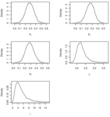
The lower panel of Table 4 reports the posterior summary statistics of the maximum a posteriori
model, and Figure 1 shows the corresponding marginal posterior densities. The data appear to be
particularly informative in all these parameters. That is, the variances of the marginal posterior
distributions are found to be systematically smaller than the prior variances. The marginal priors
seem to have only negligible influence on the marginal posteriors. The fact that our results are very
similar to the maximum likelihood (ML) estimates of Lanne and Saikkonen (2008) also attests to
this. However, the posterior median of the degrees of freedom parameter ν (4.5) differs from its
ML estimate (3.7) because its posterior density is skewed to the right. From the graph of the
marginal posterior density of ν in Figure 1 the posterior mode is seen to be fairly close to its ML
estimate.
6.2. Forecasting exercise
As pointed out above, forecasts are easily obtained as a by-product of Bayesian estimation of
noncausal AR models. Out-of-sample forecasting is one of the major uses of univariate time series
models, and, therefore, it is of interest to compare the forecasting performance of both noncausal
AR models and a number of other models suggested for inflation series in the previous literature.
Forecast horizons from one to four quarters are considered (h = 1, 2, 3, 4).
We employ the following recursive forecasting procedure for the Bayesian AR models: J different
models (j = 1,…,J) are estimated on demeaned data from the in-sample period (t = 1,…,T), their
marginal likelihoods are calculated, and, using equation (10), the predictive densities over
yT+1,…,yT+h are computed using two alternative model selection strategies described below. Moving
forward, the data for period t = 1,…,T+1 are demeaned, all models are re-estimated, their marginal
likelihoods are calculated and the predictive densities over yT+2,…,yT+h+1 are computed. This is
continued until the end of our time series. The period over which the dynamic forecast distributions
are computed in this manner is 1984:1 through 2006:3.8 This period is particularly interesting
8
In the recursive forecast exercise, a total of 92 chains for each combination of s and r are simulated (rmax = smax = 4,
thus, altogether 2300 chains). The posterior estimates of ε-, ε+ and θ are based on 50,000 draws, and the first 10,000
because, according to Atkeson and Ohanian (2001) and Stock and Watson (2007), for the U.S. the
forecasts based on standard multivariate forecasting methods have been found inferior to the naïve
forecast based on the univariate random walk since 1984.
Two alternative strategies are applied in model selection at each step. In the first approach, posterior
model probabilities are used to select the optimal lead and lag lengths, and forecasts are generated
from the selected model, referred to as AR(rm, sm). In the alternative strategy, the effect of model
uncertainty is controlled by Bayesian model averaging (BMA). In particular, the posterior
predictive density of the future observation yT+h is an average of the posterior predictive densities of
yT+h of the J models being considered, weighted by their posterior model probabilities (see e.g.
Hoeting et al., 1999). In other words, the predictive density is obtained as
J
j T h j j
h
T p y M p M
y p
1 y, y
y . (23)
This approach obviously takes into account the uncertainty in model selection by marginalizing out
the unknown models (in our case the quantities r and s). In both approaches the posterior median
forecasts are used as a point forecasts. The results based on the posterior means (not reported)
turned out to be very close to those based on posterior medians.
The predictive performance of noncausal and causal Bayesian models is compared to that of the
naïve model, the classical first-order integrated moving average (IMA(1,1)) model, suggested by
Nelson and Schwert (1977) for inflation, and the conventional classical causal autoregressive model
where the optimal lag length is determined by the Akaike Information Criterion (AIC). The naïve
forecast we consider is given by the average annualized quarterly inflation over the previous h
quarters. The IMA(1,1) model, in turn, is given by
tt L
y
1 , (24)
where ω is a parameter to be estimated and ηt is a normally distributed error term (see Stock and
Watson, 2007, and the references therein). As Nelson and Schwert (1977) and Fama and Gibbons
(1984), among many others, point out, the sample autocorrelations of U.S. inflation suggest a first-
the marginal likelihoods and every 20th draw is used in the calculation of the predictive distributions. The convergence
order moving average process as a model for Δyt, as given in equation (24). On the other hand,
because the first autocorrelation coefficient of yt estimated from our data is roughly 0.6 and the
higher-order coefficients decline slowly, a causal AR(r,0) model could be a suitable time series
model for the level of inflation. We use the Akaike Information Criterion (AIC) to select the order
of this classical causal AR(r,0) model at each step and refer to it as the AR(raic,0) model.
The commonly used measure of forecasting accuracy, the root mean squared forecast error (RMSE)
is applied for the h-step-ahead forecast errors eT(h) = yT,T+h – yT,T+h|T, where yT,T+h|T is a point forecast
of yT,T+h (such as posterior median), and yT,T+h is the average annualized quarterly inflation over the
h quarters. Table 5 shows the RMSEs of the forecasting models relative to the benchmark
AR(raic,0) model. In addition to the entire out-of-sample period, the forecasts are compared for the
1984:1 - 1994:2 and 1994:3 - 2006:4 subsample periods of equal length. This allows us to control
for the possible structural break in the mid 1980s. The out-of-sample forecasts indicate the
superiority of noncausal AR models over the alternatives. The AR(rm, sm) forecast performs very
well in all out-of-sample periods and at all forecasting horizons. However, the differences in favor
of the noncausal model seem to increase with the forecast horizon. Interestingly, model averaging
performs noticeably better only in the most recent period, having the lowest RMSEs at all
forecasting horizons. Otherwise, it yields similar or slightly less accurate forecasts than the
AR(rm,sm) model. Finally, improvement of the one-year-ahead naïve forecasts over the IMA(1,1)
and AR(raic,0) forecasts is smaller in our paper than in Stock and Watson (2007), which suggests
that our benchmark models are well specified.
7. Conclusion
In this paper, we have introduced Bayesian techniques to analyze the dynamics of economic time
series in which expectations play an important role. In particular, we have studied the noncausal AR
models, which allow for dependence on future as well as past values of the variable in question,
from the perspective of model selection. In addition, we have shown how to generate forecasts from
noncausal AR models in a straightforward manner.
We examined the finite-sample properties of our model selection procedure by means of simulation
experiments. In general, our results indicate that the Bayesian posterior model probability criterion
is able to discriminate between causal and noncausal specifications fairly well. In particular, the
of noncausality. Furthermore, when the true data generating process is causal, the Bayesian criterion
selects the noncausal model markedly less frequently than the classical procedure of Breidt et al.
(1991) and Lanne and Saikkonen (2008). Thus, it seems that the probability of falsely selecting a
noncausal process is lower with the Bayesian criterion. However, although Bayesian model
selection works well, it has difficulties in discriminating between causal and noncausal
specifications when the true model is a first-order causal or purely noncausal process with a near
unit root, in which case the noncausal and causal models are almost indistinguishable.
The methods introduced in this paper were applied to U.S. consumer price inflation. The results
show that the observed persistence in inflation is caused by the predictability of inflation instead of
economic agents' relying on past inflation in forming expectations. However, we also found some
evidence of the backward-looking behavior of agents, which contradicts typical New Keynesian
models with forward-looking dynamics, but accords with much of recent empirical literature.
Finally, our forecasting results indicate that the forecasts based on noncausal AR models are, in
References
Andrews, B., R.A. Davis, and F.J. Breidt (2006). Maximum likelihood estimation for all-pass time
series models. Journal of Multivariate Analysis 97, 1638–1659.
Atkeson, A., and L.E. Ohanian (2001). Are Phillips curves useful for forecasting inflation?. Federal
Reserve Bank of Minneapolis Quarterly Review 25, 2–11.
Bauwens, L., and M. Lubrano (1998). Bayesian inference on GARCH models using Gibbs sampler.
Econometrics Journal 1, 23–46.
Bauwens, L., M. Lubrano, and J.-F. Richard (1999). Bayesian Inference in Dynamic Econometric
Models, Oxford University Press.
Breidt, J., R.A. Davis, K.S. Lii, and M. Rosenblatt (1991). Maximum likelihood estimation for
noncausal autoregressive processes. Journal of Multivariate Analysis 36, 175–198.
Breidt, J., R.A. Davis, and A.A. Trindade (2001). Least absolute deviation estimation for all-pass
time series models. Annals of Statistics 29, 919–946.
Campbell, J.Y., and N.G. Mankiw (1990). Permanent income, current income, and consumption.
Journal of Business and Economic Statistics 8, 265–79.
Fama, E. F., and M. R. Gibbons (1984). A comparison of inflation forecasts. Journal of Monetary Economics 13, 327–348.
Galí, J., and M. Gertler, (1999). Inflation dynamics: A structural econometric analysis. Journal of
Monetary Economics 44, 195–222.
Galí, J., M. Gertler, and J.D. López-Salidod (2005). Robustness of the estimates of the hybrid New
Keynesian Phillips curve. Journal of Monetary Economics 52, 1107–1118.
Gelfand, A., and D. Dey (1994). Bayesian model choice: Asymptotic and exact calculations.
Gelman, A., J.B. Carlin, H.S. Stern and D.B. Rubin (2004). Bayesian Data Analysis, 2nd edition,
Chapman & Hall/CRC.
Geweke, J. (1992). Evaluating the accuracy of sampling-based approaches to calculating posterior
moments. In Bernado, J.M., J.O. Berger, A.P. Dawid, and A.F.M. Smith (eds.) Bayesian Statistics
4, Clarendon Press, Oxford, UK.
Geweke, J. (1993). Bayesian treatment of the independent Student-t linear model. Journal of
Applied Econometrics 8, 19–40.
Geweke, J. (1999). Using simulation methods for Bayesian econometric models: Inference,
development and communication. Econometric Reviews 18, 1–126.
Hoeting, J.A., D. Madigan, A.E. Raftery, and C.T. Volinsky (1999).Bayesian model averaging: A
tutorial. Statistical Science 14, 382–417.
Huang, J., and Y. Pawitan (2000). Quasi-likelihood estimation of noninvertible moving average
processes. Scandinavian Journal of Statistics 27, 689–710.
Koop, G. (2003). Bayesian Econometrics. Wiley.
Lanne, M., and P. Saikkonen (2008). Modeling expectations with noncausal autoregressions.
HECER Discussion Paper No. 212.
Marriott, J., and P. Newbold (2000). The strength of evidence for unit autoregressive roots and
structural breaks: A Bayesian perspective. Journal of Econometrics 98, 1–25.
Nelson, C.R., and G.W. Schwert (1977). Short-term interest rates as predictors of inflation: On
testing the hypothesis that the real rate of interest is constant. American Economic Review 67, 478–
486.
O'Hagan, A. (1995). Fractional Bayes factors for model comparison. Journal of the Royal Statistical
Rudd, J., and K. Whelan (2006). Can rational expectations sticky-price models explain inflation
dynamics? American Economic Review 96, 303–320.
Smets, F., and R. Wouters (2007). Shocks and frictions in US business cycles: A Bayesian DSGE
approach. American Economic Review 97, 586–606.
Stock, J.H., and M. Watson (2007). Why has U.S. inflation become harder to forecast?
Table 1. Simulation results for Student prior and multivariate Normal prior.
___________________________________________________________________________________________________________________________
DGP
_______________________________________________________________________________________
1 . 0
1
1 0.7 1 0.7 1 0.1 1 0.7 1 0.7
_______________________________________________________________________________________
Parameter Mean St. dev. Mean St. dev. Mean St. dev.
____________________________________________________________________________________________________________________________
Posterior mode
Student prior 1
0.100 0.079 0.678 0.057 0.690 0.061
1
0.680 0.062 0.106 0.072 0.687 0.062
____________________________________
Posterior mode
Normal prior 1
0.103 0.084 0.684 0.067 0.687 0.064
1
0.681 0.066 0.101 0.080 0.690 0.064
____________________________________
ML estimator
1
0.102 0.086 0.681 0.067 0.686 0.067
1
0.687 0.067 0.108 0.081 0.692 0.067
___________________________________________________________________________________________________________________________
The DGP is the AR(1,1) model where the error term follows the t-distribution with ν = 3 and σ = 1. The results
Table 2. Mean of p(M4|y) and proportion of times when p(M4|y) > 0.5.
Panel A. The mean of p(M4|y)
_________________________________________________________________________
1
_____________________________________________________________________________________________
1
0.1 0.3 0.5 0.7 0.9 0.99
_________________________________________________________________________________________________________________________
0.0 0.18 0.29 0.30 0.25 0.20 0.11
0.1 0.26 0.45 0.49 0.45 0.39 0.24
0.3 0.44 0.84 0.91 0.95 0.95 0.77
0.5 0.45 0.92 0.99 1.00 1.00 0.99
0.7 0.40 0.93 1.00 1.00 1.00 1.00
0.9 0.27 0.89 1.00 1.00 1.00 1.00
0.99 0.15 0.76 0.99 1.00 1.00 1.00
_____________________________________________________________________________________________________________
Panel B. Proportion of times when p(M4|y) > 0.5
___________________________________________________________________________
1
_____________________________________________________________________________________________
1
0.1 0.3 0.5 0.7 0.9 0.99
_________________________________________________________________________________________________________________________
0.0 0.06 0.12 0.13 0.09 0.07 0.06
0.1 0.11 0.37 0.44 0.36 0.33 0.22
0.3 0.36 0.89 0.93 0.97 0.97 0.77
0.5 0.41 0.95 0.99 1.00 1.00 0.98
0.7 0.35 0.96 1.00 1.00 1.00 1.00
0.9 0.23 0.91 1.00 1.00 1.00 1.00
0.99 0.10 0.77 0.99 1.00 1.00 1.00
______________________________________________________________________________________________________________
The DGP is the AR(1,1) model where the error term follows the t-distribution with ν = 3 and σ =