Computer Science Dissertations Department of Computer Science
Summer 7-13-2010
Energy-Efficient Data Management in Wireless Sensor Networks
Energy-Efficient Data Management in Wireless Sensor Networks
Chunyu Ai
Georgia State University
Follow this and additional works at: https://scholarworks.gsu.edu/cs_diss
Part of the Computer Sciences Commons
Recommended Citation Recommended Citation
Ai, Chunyu, "Energy-Efficient Data Management in Wireless Sensor Networks." Dissertation, Georgia State University, 2010.
https://scholarworks.gsu.edu/cs_diss/55
This Dissertation is brought to you for free and open access by the Department of Computer Science at
by
CHUNYU AI
Under the Direction of Dr. Yingshu Li
ABSTRACT
Wireless Sensor Networks (WSNs) are deployed widely for various applications. A variety
of useful data are generated by these deployments. Since WSNs have limited resources and
unreliable communication links, traditional data management techniques are not suitable.
Therefore, designing effective data management techniques for WSNs becomes important.
In this dissertation, we address three key issues of data management in WSNs.
For data collection, a scheme of making some nodes sleep and estimating their values
according to the other active nodes’ readings has been proved energy-efficient. For the
Most of existing data processing approaches of WSNs are real-time. However, historical
data of WSNs are also significant for various applications. No previous study has specifically
addressed distributed historical data query processing. We propose an Index based Historical
Data Query Processing scheme which stores historical data locally and processes queries
energy-efficiently by using a distributed index tree.
Area query processing is significant for various applications of WSNs. No previous study
has specifically addressed this issue. We propose an energy-efficient in-network area query
processing scheme. In our scheme, we use an intelligent method (Grid lists) to describe an
area, thus reducing the communication cost and dropping useless data as early as possible.
With a thorough simulation study, it is shown that our schemes are effective and
energy-efficient. Based on the area query processing algorithm, an Intelligent Monitoring System
is designed to detect various events and provide real-time and accurate information for
escaping, rescuing, and evacuation when a dangerous event happened.
by
CHUNYU AI
A Dissertation Submitted in Partial Fulfillment of the Requirements for the Degree of
Doctor of Philosophy
in the College of Arts and Sciences
Georgia State University
by
CHUNYU AI
Committee Chair: Dr. Yingshu Li
Committee: Dr. Yi Pan
Dr. Raheem Beyah
Dr. Xu Zhang
Electronic Version Approved:
Office of Graduate Studies
College of Arts and Sciences
Georgia State University
DEDICATION
ACKNOWLEDGEMENTS
I would like to thank all of those people who helped make this dissertation possible.
First of all, thank my advisor, Dr. Yingshu Li, for all her guidance, encouragement,
support, and patience. Dr. Li was always there to listen and to provide constructive advice.
She taught me how to express my ideas and showed me different ways to approach a
re-search problem. During difficulty times of my life, she understood my situation and totally
supported me. Without her guidance and persistent help this dissertation would not have
been possible.
I would like to thank my committee members, Dr. Yi Pan , Dr. Raheem Beyah, and
Dr. Xu Zhang, for their very helpful insights, comments, and suggestions. Dr. Pan proposed
thoughtful suggestions for improving my dissertation. Dr. Beyah taught me how to write
an academic paper, guided me to solve the research issues, and provided me useful materials
and information. Many thanks also goes to Dr. Raj Sunderraman who instructed me Ph.D.
study and teaching.
A special thanks goes to Prof. Jianzong Li, my advisor of M.S., who brought me in the
research field in the first place and encouraged me to pursue the Ph.D. degree.
In addition, I would like to thank my fellow graduate students and postdoc, Dr.
Longjiang Guo, Yiwei Wu, Shan Gao, Chinh T. Vu, Jing He, Souling Ji, and Yueming
Duan, who provided invaluable support and suggestions throughout this process. Thank my
friends for sharing happiness.
Last, but not least, I thank my family: my parents, Shuqin Tian and Guozhen Ai,
for giving me life, for educating me, for unconditional supporting me. Thank my brother,
TABLE OF CONTENTS
ACKNOWLEDGEMENTS . . . v
LIST OF TABLES . . . ix
LIST OF FIGURES . . . x
LIST OF ABBREVIATIONS . . . xii
Chapter 1 INTRODUCTION . . . 1
1.1 Data Management in Wireless Sensor Networks . . . 2
1.2 Some Research Issues of Data Management in WSNs . . . 4
1.2.1 Data Estimation Using Physical and Statistical Methodologies . . 4
1.2.2 In-network Historical Data Storage and Query Processing . . . 5
1.2.3 Area Query Processing . . . 7
Chapter 2 RELATED WORK . . . 10
2.1 Basic Approaches to Data Management in WSNs . . . 10
2.2 Data Collection and Estimation . . . 11
2.3 Data Storage . . . 13
2.4 Area Query . . . 15
Chapter 3 DATA ESTIMATION USING PHYSICAL AND STATIS-TICAL METHODOLOGIES . . . 18
3.1 Problem Definition and Working Scenario . . . 18
3.2 Estimation Models . . . 19
3.2.2 Data Estimation using Statistical Model (DESM) . . . 24
3.2.3 Discussion . . . 26
3.3 Experiment Results . . . 28
3.3.1 Estimation accuracy . . . 30
3.3.2 Energy consumption . . . 32
Chapter 4 IN-NETWORK HISTORICAL DATA STORAGE AND QUERY PROCESSING . . . 35
4.1 Historical Data Storage . . . 35
4.2 Construct and Maintain Distributed Index Tree . . . 36
4.2.1 Construct a Hierarchical Index Tree . . . 36
4.2.2 Index Maintaining . . . 39
4.3 Historical Data Query Processing . . . 40
4.4 Multi Query Optimization . . . 42
4.5 Simulation . . . 44
Chapter 5 AREA QUERY PROCESSING . . . 51
5.1 Area Query in Wireless Sensor Networks . . . 51
5.2 In-network Area Query Processing Scheme . . . 53
5.2.1 Area Partition . . . 53
5.2.2 Reporting Tree Construction . . . 56
5.2.3 In-network Area Query Processing . . . 57
5.2.4 Incremental Result Update . . . 62
5.2.5 Advantages of Using Gray Codes . . . 63
5.3 Intelligent Monitoring Systems . . . 63
5.3.1 Escaping Routing Algorithm . . . 66
5.4 Simulation Results . . . 66
5.4.2 Efficiency of Our Scheme . . . 68
Chapter 6 CONCLUSIONS . . . 73
LIST OF TABLES
Table 3.1 Symbol Table . . . 22
Table 3.2 System Parameters and Setting. . . 32
Table 3.3 Model Selection Guideline. . . 33
LIST OF FIGURES
Figure 1.1 Area Queries . . . 7
Figure 3.1 Working rounds. . . 19
Figure 3.2 A light intensity monitoring WSN. . . 21
Figure 3.3 A Grid. . . 25
Figure 3.4 Experimental environment. . . 29
Figure 3.5 The relative error of estimations reported by DEPM and DESM using data set 1. . . 30
Figure 3.6 The relative error of estimations reported by DEPM and DESM using data set 2. . . 31
Figure 3.7 The relative error of estimations reported by DEPM and DESM using data set 3. . . 31
Figure 3.8 The energy consumptions of different models. . . 34
Figure 3.9 The remained energy of DEPM. . . 34
Figure 4.1 Network Partition . . . 36
Figure 4.2 Index Tree . . . 37
Figure 4.3 Index tree on BS. . . 44
Figure 4.4 Cost of maintaining the index tree with various network size. . . . 45
Figure 4.5 Query responding delay of variant network size. . . 46
Figure 4.7 Total network traffic of variant network size. . . 47
Figure 4.8 Average network traffic of variant average involved nodes percentage of queries. . . 47
Figure 4.9 Average network traffic of variant average length of query time win-dow. . . 48
Figure 4.10 Accumulative network traffic of . . . 48
Figure 5.1 Working Scenario. . . 54
Figure 5.2 Merge subareas. . . 59
Figure 5.3 IMS for monitoring fire in a building. . . 64
Figure 5.4 Network Traffic of execution intervals (L=10 bits, S=50%, F=50%, C=20%). . . 69
Figure 5.5 Network Traffic of variantL(S=50%,F=50%,C=20%, 100intervals). 69
Figure 5.6 Network Traffic of variantS(L=10bits,F=50%,C=20%, 100intervals). 70
Figure 5.7 Network Traffic of variantF (L=10bits,S=50%,C=20%, 100intervals). 70
LIST OF ABBREVIATIONS
• WSN - Wireless Sensor Network
• BS - Base Station
Chapter 1
INTRODUCTION
A Wireless Sensor Network (WSN) is a wireless network composing of spatially
dis-tributed sensor nodes. Each sensor node is normally small, lightweight, and portable. A
sensor node in a WSN is typically equipped with a transducer, a radio transceiver, a small
microcontroller, and a power source (usually batteries). The transducer can convert sensed
physical effects and phenomena into electrical signals. Consequently, sensor nodes can
coop-eratively monitor physical or environmental conditions to collect, record, and report data and
information of monitored objects. Generally, monitored parameters are temperature,
humid-ity, wind direction, speed, illumination intenshumid-ity, sound intenshumid-ity, vibration intenshumid-ity,
pres-sure, power-line voltage, chemical concentrations, motion, pollutant levels, and vital body
functions. The microcontroller processes and stores the sensed data. The radio transceiver
is responsible for receiving and sending data packets from/to other sensor nodes and BS.
Also, each sensor supports a multi-hop routing algorithm, so a packet can be received by the
destination node through multi-hop forwarding. The size of a single sensor node can vary
from the size of a shoebox down to grain. Moreover, a sensor node costs from hundreds of
dollars to a few pennies, depending on the size and the complexity requirements. Due to
size and cost constraints of sensor nodes, there are corresponding constraints on resources
including computational capability, memory capacity, energy, and bandwidth [1].
Initially, WSNs were designed for military applications such as battlefield surveillance.
Nowadays WSNs are widely used in many civilian and industrial application areas, such as
industrial process monitoring and control, machine health monitoring, robot control,
envi-ronmental monitoring, habitat monitoring, healthcare applications, home automation, object
tracking, detecting disasters, and traffic control. In the recent years, WSNs have entered a
[2]. WSNs has attracted many researchers’ attention in the field of computer science and
telecommunications, and there are numerous workshops and conferences arranged each year.
1.1 Data Management in Wireless Sensor Networks
Nowadays large-scale sensor networks are widely deployed around the world for various
applications. Tremendous volumes of various useful data are generated by these deployments.
An interface between WSNs and users, which can extract the data users want and represent
the data as the format users required, is significant. To develop this kind of interface, it is
in-dispensable of supporting of data management techniques. However, compared to traditional
networks or databases, a WSN has limited storage capacity, processing, analysis,
computa-tion abilities, bandwidth, and power supply. Obviously, tradicomputa-tional data management and
processing methods are not suitable for WSNs. Thus, how to collect, store, process, and
an-alyze data generated by WSNs is a challenging issue. In the past years, researchers proposed
a lot of systems, algorithms, and methods to address data management problems of WSNs
such as data collection, various aggregations, queries processing, event detection, and data
mining. When we design algorithms for WSNs, the following are several characteristics and
constraints of sensors and WSNs we have to consider.
1. Unstable and unreliable. The network topology of WSNs change frequently due to the
following reasons:
(a) Some sensor nodes have mobility.
(b) New sensor nodes join in.
(c) Some sensor nodes leave because of using up energy.
Moreover, wireless communication is unreliable in practice since wireless channel is
not reliable especially compared to wired channel. Due to practical issues such as link
failures, high retransmission rate, and high packet missing rate, 100% communication
2. Limited power supply. Due to the constraint of deployment environment, sensor nodes
generally use batteries as power supply instead of wired power supply. For instance,
the popular motes, Mica2, Micaz, and TelobB, use 2 AA batteries [3]. Normally,
the lifetime of batteries can be several weeks or months [4]. Unfortunately, for some
sensor nodes which are deployed at dangerous environment or unreachable spots,
re-placing the batteries is not possible. Therefore, prolonging the network lifetime is an
important optimization goal for designing an algorithm of WSNs. Also, the network
lifetime or energy consumption is usually used to judge the performance of an
algo-rithm. Importantly, the communication operations, such as sending, receiving, and
forwarding packets, are the most energy consumed operations compared to sensing,
computing, etc. The energy consumption for transmitting 1 Kb a distance of 100 m is
approximately the same as that for the executing 3 million instructions by 100 million
instructions per second/W processor [5]. Thus, reducing unnecessary communication
cost is an efficient way to save energy and prolong the network lifetime. Therefore, we
only consider the communications cost (network traffic) when we evaluate the energy
efficiency of the designed algorithms.
3. Low bandwidth. The bandwidth of WSNs is low because of the constraints of wireless
radio,power supply, and other charactoristcs of WSNs. The transmit data rate of Micaz
and TelobB’s wireless transceiver is 250 kbps [3]. However, the bandwidth of WSNs
cannot reach a sensor’s maximum bandwidth since low qualify links, collisions, and
high retransmission rate due to packets missing affect the transmission performance of
WSNs. Moreover, for large-scale WSNs, the transmission latency is high since WSNs
must use multi-hop routing mechanism due to the limited transmission range of a
wireless transceiver.
4. Limited storage capacity and computational ability. The storage capacity and
com-putation ability of a sensor node is restricted by the requirements of size and cost.
48K bytes program flash memory, 10K bytes RAM, and 1024K bytes measurement
serial flash memory [3]. Therefore, the processing and storing ability of a single sensor
node is limited. However, the ability of a WSN is powerful by making all sensor nodes
cooperate with each other.
Aforementioned constraints of WSNs make designing data management algorithms more
challenging.
1.2 Some Research Issues of Data Management in WSNs
In this section several research issues of data management in WSNs, which are addressed
in my dissertation, are introduced.
1.2.1 Data Estimation Using Physical and Statistical Methodologies
Sensor-based applications extract different kinds of data via collecting data, processing
in-network aggregations, and detecting complicated events. Since sensor nodes have limited
resources, novel data management techniques are needed to satisfy application requirements,
especially, the limitation of resources. To date, data acquisition using WSNs has became
an essential ingredient of current technologies. Due to the energy limitations faced by
sen-sor nodes, most techniques focus on in-network aggregating data so as to improve energy
efficiency. Although this is a good way to conserve energy, for some applications it is
neces-sary that all sensor readings are collected by BS. In such a scenario,in-network aggregation
cannot be permitted as it reduces the data-set communicated to BS. Consequently, in such
situations, data-estimation can prove to be a very fruitful alternative to data aggregation.
An example is the determination of light intensity distribution in a region, such as
photosen-sitive horticulture under artificial illumination [6]. Commercial gadgets are now available [7]
for such purposes, the HortiSpec [7] was developed to measure light intensity and spectral
distribution in the visible and NIR range inside greenhouses. The light intensity can be
would help conserve energy and prolong network lifetime. Commercial light sensors which
use photodiodes that produce a voltage proportional to the light intensity are now available.
Similarly, light intensity sensors are required to monitor maintenance of optimum lighting in
animal husbandry related business [8], and also in cell-culture experiments [9] under artificial
light, where also data estimation techniques would help enhance the longevity of WSNs.
Usually, users can accept approximate data. As a result, a method of data estimation
is a perfect option for conserving energy. In fact, the key challenge is how to provide
estimated data with high precision while consuming as little energy as possible. To address
this problem, two novel data estimation methods are proposed in Chapter 3. In our scheme,
a minimal number of nodes are set to be active and the other nodes are set to sleep. All nodes
serve as active working nodes by turns. BS estimates values of sleeping nodes based on two
estimation models, Data Estimation using Physical Model (DEPM) and Data Estimation
using Statistical Model (DESM). The scheme not only prolongs network lifetime, but also
fulfills users’ expectations of data precision. Notably, the DEPM model is the first one to take
advantages of physical characteristics of monitored attributes for estimation. Experiments
on a real sensor network consisting of twenty TelosB nodes [10] were conducted to evaluate
the proposed models. The experimental results show that the proposed methods are energy
efficient.
1.2.2 In-network Historical Data Storage and Query Processing
Most existing applications just process real-time data generated by WSNs (e.g., [11, 12]).
However, historical data of sensor networks are also significant to us, especially statistical
meaning of historical data. For instance, maximum, minimum, and average temperatures
of the past two months in a specific area are concerned in the weather monitoring
applica-tion. By capturing rush hours and the bottleneck of traffic according to historical data, a
large quantity of useful information can be provided to improve traffic conditions. Through
analysis of historical data, some knowledge, principles, and characteristics can be discovered.
a centralized manner. Nevertheless, sensor nodes will deplete energy rapidly for continually
reporting and forwarding data. Another method is storing data locally, that is, data are
stored at a sensor node where they are generated. Intuitively, a sensor node cannot store
a large quantity of historical data since its memory capacity is low. Popular motes such as
Mica2 and Micaz [3] are equipped with a 512K bytes measurement flash memory, it can store
more than 100,000 measurements. Another popular mote, TelosB [3], has a 1024K bytes flash
memory. 512K or 1024K bytes are really small memory capacity. However, it is enough to
store most of sensing data, sampling data, or statistical data during a sensor node’s entire
lifetime since the lifetime of a sensor node is short due to the limitation of batteries. For a
Mica mote powered by 2 AA batteries, the lifetime is 5-6 days if continuously running, and
it can be extended to over 20 years if staying sleep state without any activity [13]. For most
applications, a sensor can live for several weeks or months [4]. Assume a Mica mote with
a 512K bytes flash memory can live 3 months. (100,000/90) = 1111 measurements can be
saved locally every day. Suppose we have 4 sensing attributes need to be saved, frequency
of sampling can be 1 per 5 minutes which is normal in wireless sensor network applications.
If proper compressing techniques are applied according to data’s characteristics, much more
data can be stored locally. Consequently, storing data locally at a sensor is feasible. The
historical data can be downloaded when the battery is replaced or recharged if possible.
The motivation of storing historical data is to support historical data queries. However,
locally storing data might cause a query to be flooded in the entire network to probe data
when it is processed. We propose a scheme in Chapter 4 named Historical Data Query
Processing based on Distributed Indexing (HDQP) which stores historical data in network
and processes queries energy-efficiently by using index techniques. Historical data is stored at
each sensor. For saving memory capacity, compressing and sampling techniques can be used
according to data characteristics and users’ requirements. To process queries quickly and
energy-efficiently, in-network distributed tree-based indexes are constructed. Using indexes
to process queries can reduce the number of involved sensors as many as possible, thus
nodes according to their time stamp. That is, there exist multiple index trees in the network.
Which index trees are used depends on query conditions.
1.2.3 Area Query Processing
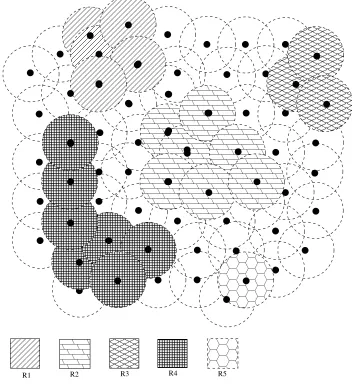
[image:22.612.128.480.191.577.2]R1 R2 R3 R4 R5
Figure 1.1. Area Queries
Most existing data collection systems are query-based ones. Traditional query processing
techniques of WSNs mainly deal with retrieving sensor node locations, sensing values, and
aggregating the sensed values. However, in a lot of applications, users expect information
a high oxygen density to take a break, and this area must be big enough to accommodate
several workers. In Figure 1.1, all sensing values of the sensors in regions R1 through R5 reach
the expected oxygen density. However, regions R3 and R5 are not big enough for several
workers, so R3 and R5 are not the areas users expect. For this application, previous methods
may only return the locations and sensing values of the sensors, which is meaningless and
helpless. Here, users want to find areas instead of several locations since the size of an area
should also be a filtering condition.
Another interesting scenario is an air pollution monitoring application within a city.
Users expect this monitoring system to detect regions whose pollution levels reach thresholds.
In reality, the polluted thresholds might be different for different areas. For example, the
threshold of an industrial area is 80, and that of a residential area is 50. In Figure 1.1,
R1 and R4 are in the industrial area, and R2, R3, and R5 are in the residential area. The
polluted level of R1 through R5 are 70, 60, 40, 90, and 40 respectively. Usually, traditional
methods apply the same filtering condition for the whole network. In this example, if the
threshold 80 is used, polluted area R2 is missed since R2’s polluted level actually exceeds
the threshold for residential areas while the filtering condition does not indicate this. If the
threshold 50 is used, R1 is identified as a polluted area which triggers a false alarm. So
the existing methods cannot be used for this application. This application concerns specific
areas, and different filtering conditions should be applied for each area.
We define Area Query as requests for area information including area locations, sizes
of areas, and collected and aggregated data of areas. Sensor nodes with expected readings
and adjacent sensing coverage are divided into the same group. The total coverage area of
sensor nodes in the same group is a possible result area. Area Query can retrieve not only
sensing values but also specific geographical information compared to traditional queries of
wireless sensor networks. Area Query is more practicable and useful than traditional queries
for some applications, which require geographical information. A common property of Area
Query applications is that results of these queries are areas and aggregation values of sensors
for either the whole network or sub-areas. For different areas, it is possible to use different
querying conditions. Area Query is a new kind of query in wireless sensor networks.
Intuitively, BS can collect data from all sensor nodes and answer area queries. However,
sensor nodes will drain energy quickly due to frequently reporting. Existing techniques of
in-network query processing suppress and aggregate sensing values to save energy. However,
these methods do not consider sensor coverage area as part of results. Consequently, a new
in-network area query processing technique is necessary.
The first challenge of in-network area query processing is that it is hard to suppress
useless data as early as possible. For instance, an area satisfies all the conditions except size
of requirement. Obviously, this area is not the one expected by users. However, we cannot
drop this area since it is difficult to decide the boundary of a result area locally. Moreover,
how to describe an area in-network is another challenge. Because areas are also part of query
results, ideal area description can reduce the size of transmitted data and the complexity of
area size computation, which are two primary consideration factors for energy conservation.
In Chapter 5, we propose an energy-efficient in-network area query processing scheme.
The whole sensor network is partitioned into grids, and a gray code is used to represent
each grid. We construct a reporting tree to process merging areas and aggregations. For
conserving energy, incremental update techniques are used to process continuous queries.
Our contributions are summarized as follows:
1. A new area query is studied.
2. A smart area description, GID lists, is used to reduce the size of query results.
3. An energy-efficient in-network area query processing scheme is proposed. By using
GIDs and merging strategies, partial results can be merged to reduce the size of results
and useless data can be dropped as early as possible to reduce the number of messages.
4. An incremental update method is addressed to reduce the size of reports for continuous
Chapter 2
RELATED WORK
In this chapter, we begin with a brief introduction of related work to data management
in WSNs. Then, related literature of research issues which are addressed in the dissertation
is discussed.
2.1 Basic Approaches to Data Management in WSNs
First, we introduce some early data management approaches. In [14], a scalable and
robust communication paradigm, directed diffusion, is proposed. Attribute-value pairs are
used to name data generated by sensor nodes. A request node sends its interests of named
data to destination sensor nodes or regions. Then, data satisfying the interest are returned
along the reverse path of interest dissemination to the request node. To improve the
perfor-mance and save energy, intermediate nodes can cache data and might aggregate the data.
[15] extends and improves the directed diffusion method especially on experiments. TinyOS
[16] is a free and open source operating system designing for WSNs. TinyOS is an embedded
operating system which is written in the nesC. The component library of TinyOS consists of
sensor drivers, network protocols, distributed services, and data acquisition tools. Therefore,
TinyOS can support basic data requests. Moreover, users can develop their own applications
based on TinyOS.
TinyDB [4] is a data management system for WSNs based on TinyOS. It can extract
information from WSNs by sending queries. Importantly, TinyDB allows users describe
the data they want to acquire by writing a simple, SQL-like query. For answering a query,
TinyDB requests the data from sensor nodes in the network and routes it back to a PC. In the
phase of processing queries, filtering and aggregation algorithms might be used. TinyDB uses
For instance, tree-based routing is used for query delivery, data collection, and in-network
aggregation, and [17] is used to processing aggregation in in-network manner. Also, TinyDB
supports metadata management, in-network persistent storage, multiple concurrent queries.
REED [18] extends TinyDB with the ability to process joins operations between sensing data
and static tables which is built outside the WSN. Filter conditions is stored in static tables,
and then those tables are distributed throughout the network. Join operation is executed
in in-network manner. REED is also suitable for various event detection applications which
TinyDB and data collection systems cannot handle.
Cougar [19] is another distributed database system to sensor networks. It
consid-ered query languages, aggregation processing, query optimization, catalog management, and
multi-query optimization. When a new query is coming, query optimizer of Cougar either
merge it with an existing query or generate a new query plan. A leader is chosen to control
the execution of the query plan.
Recently, researchers focus on specific issues which were found in some applications
such as data estimation, data aggregation, event detection, and data centric storage. In the
following sections we will introduce literature which is related to the issues we focus on.
2.2 Data Collection and Estimation
Common techniques to save energy in WSNs employ various alternative strategies to
minimize data acquisition and/or transmission by using a variety of approaches. For
in-stance, in-network aggregation (e.g., MIN [20] and AVG [17]) can reduce communication
cost significantly. Also, using synopsis diffusion [21] and wavelets compression [22] to
pre-cess aggregation can decrease network traffic. However, aforementioned methods are not
suitable for some applications which require all sensed data to be sent to BS since these
methods do not provide detailed data desired by users. Apparently, reporting all sensed
data will consume energy quickly. Therefore, researchers proposed some energy-efficient
approximate algorithms to collect all sensed data.
contin-uously (SELECT ∗ query). In [23], Chu et al. have proposed a mechanism, Ken, using
conditional data transmission to conserve energy by reporting only if the difference between
the sensed value and the predicted value is beyond certain bounds. The replicated dynamic
probabilistic model for a sensor node is installed on both the sink and that sensor node. A
sensor node does not need to report sensed value normally if the predicted error is within the
threshold user specified, thus saving reporting communication cost. Once the predication
error is greater than the error bound, the sensed data is reported to the sink, and the
param-eters of the model are adjusted to match current data changing intend. The effectiveness of
this scheme in reducing the communication cost is relied on the predication model chosen.
As shown in [24], the prediction models based on the temporal and spatial correlations of
data work extremely well in WSNs. A novel disjoint-Cliques Model is also proposed to use
spacial correlation to reduce data transmission and improve prediction accuracy. In [25],
a data-driven approach was presented. Model-based suppression is used to provide
contin-uous data without contincontin-uous reporting. In addition, a key problem for data suppression,
link failure, is addressed. A mobile filtering approach for error-bounded data collection was
proposed in [26]. By migrating filters wisely the number of data reporting is reduced
signif-icantly. Jain et al. have built dynamic procedures that employ maximum filtering of data
using a technique called stochastic recursive data filtering, to conserve resources subject to
meeting precision standards [27]. Primarily, these methods are aimed at reducing energy
consumption by substituting data acquisition using data estimation. Another method of
data estimation is based on collection of data samples for a relatively long time and
cal-culating the autocorrelation of the vector of samples [28]. This approach aims at enabling
nodes to identify patterns in the behavior of sensed processes and report only uncommon
observable data to conserve energy.
Dash et al. have studied using physical laws for data estimation, approximate values
of land surface temperature and emissivity from passive sensor data [29]. Essentially, this
work makes use of well-known laws of Physics to estimate the Land Surface Temperature
govern sensor mechanisms, in the DEPM technique proposed by us in [30] it seems for the
first time that physical laws are employed in a direct energy saving strategy aimed at data
estimation. Most other methods rely on some forms of temporal and/or spatial correlations
and/or data filters for data estimation whereas in the present work well-established physical
laws that are known to be correct with extremely high accuracy are used directly in the
net-work plan to achieve minimization of energy consumption which is the primary challenge in
WSN technology. The data estimation scheme we propose can conserve more energy than the
methods mentioned above obviously, because in the methods, such as [23, 27, 28], all nodes
should be always in working status; however, in our scheme nodes serve as working nodes
by turns, and others go to sleep, so our scheme can prolong network lifetime significantly.
2.3 Data Storage
Many approaches have been proposed to describe how to store data generated by WSNs.
One category of such storage solutions is that BS collects and stores all data. Apparently,
it is easy to store and access the data at BS. However, such methods (such as [31] [17] [32])
might be more applicable to answer continuous queries. Obviously, the mortal drawback of
collecting all data is shortening the network lifetime for WSNs with limited power supply
since sending packets costs large amount of energy. Also, shipping all data out of network
may be not necessary because users are not interested in all data. Sensor nodes near BS
become the bottleneck as a result of forwarding packets. Moreover, the WSNs may not
able to transfer all data continuously generated by sensor nodes due to the limitation of
bandwidth. Since centralized storage is not practical, naturally distributed in-network data
storage is considered. Nevertheless, in-network data storage and data retrieve of WSNs are
challenging issues for WSNs because each sensor node just has limited memory space and
there are a number of sensor nodes in a WSN normally.
For improving network lifetime, in-network storage techniques have been addressed to
solve ad-hoc queries. These frameworks are primarily based on the Data-Centric Storage
meanings (e.g., tiger sightings). All data with the same general name will be stored at the
same sensor node. Then, when users query the data with a particular name, it can be sent
directly to the sensor node who stores those named data. The major difference among
in-network DCS schemes is using different events-to-sensors mapping methods. The mapping
was designed using hash tables in DHT [33] and GHT [34], or using k-d trees in DIM [35],
KDDCS [36], and STDCS [11]. STDCS uses sensor location as data indexing instead of
the sensed values. Hence, STDCS addresses a sensors-to-sensors mapping instead of the
readings/events-to-sensors mapping. Moreover, a switching-time is defined to be the time
duration after which the mapping function changes. STDCS uses a spatio-temporal indexing
to balance query load among sensors.
As we know, indexing techniques can significantly improve the data acquiring/query
performance. For WSNs, another benefit of using index is reducing cost of data request
dissemination since the destination of data request can be obtained from the index. The
works in [37], [35], and [36] use a spatially distributed hashing index technique to solve
range queries in a multi-dimensional space. The work in [12] proposed a distributed
spatial-temporal index structure to track moving objects. The work in [38] addressed a time-based
index management for event query processing. For saving energy, the index is adjusted
according to the event frequency.
Specially, most of these approaches just store partial data, which satisfy conditions or
present events and moving objects, generated by sensors [34], [36], [35], [37], [12], and [38].
To our best knowledge, no in-network distributed historical data storage, indexing, and query
processing schemes have been presented in the literature.
Since sensors have limited memory space, storing all historical data on sensors might
not be applicable for some applications with a large quantity of sensing data. However, most
applications desire statistical results, events, the trend of value changing of historical data
rather than specific values. This characteristic provides us a chance to store sketch
infor-mation to answer queries based on historical data of sensor networks. For enhancing query
forwarding. In [39], we proposed a in-network historical data storage and query processing
scheme based on distributed index. This scheme stores historical data locally and processes
queries energy-efficiently by using a distributed index tree. Regression techniques can be
used to save memory capacity according to data characteristics and users’ requirements.
In order to process queries quickly and energy-efficiently, in-network distributed tree-based
indexes are constructed and maintained. Using indexes to process queries can significantly
reduce the number of involved sensors, thus conserving energy consumption. Furthermore,
for avoiding load skew, index data are partitioned on different nodes according to their time
stamp.
2.4 Area Query
Area query processing is a special kind of data processing in wireless sensor networks.
As we know, data processing of wireless sensor networks was well-studied. It mainly involves
three aspects, data collection, data aggregation, and query processing. Resource-limitation
and unreliable communication links are the main concerns.
Data collection techniques achieve ideal data reduction when bounded error is acceptable
for users as discussed in Section 2.2. Data collection may be used to process area queries.
That is, BS computes results after collecting data from all sensor nodes. However, since
errors are not tolerable for area queries, then the methods which provide results with errors
are not suitable for area query processing. If the methods which can provide accurate results
are employed, energy consumption will be large since most of data cannot be suppressed and
must be sent to BS.
In-network data aggregation is an efficient way to reduce energy consumption since data
items are compressed on their way to the destination. TAG [17] and TiNA [40] aggregate
sensed data as early as possible through tree-based routing. Aggregation of values from
multiple sensor nodes are routed to one destination (BS). In [41], a many to many aggregation
scheme was proposed. In this scheme, there are multiple destination nodes. Each destination
Users specify a set of spatial regions, data aggregation is then performed in each region.
Existing data aggregation methods either consider the sensor nodes in the whole network as
belong to one group or divide sensor nodes into static groups such as the works in [41] and
[42]. Area query processing requires dynamic sensor grouping based on readings from each
sensor. Therefore, the above mentioned methods cannot be used.
Query processing technique involves query optimization, decomposition, distribution,
and result retrieval. A query processing system must have the ability to execute multiple
continuous queries simultaneously. Cougar [19] system reduces communication cost by
push-ing operations such as selections and aggregations into the network. TinyDB [4] is a robust
query processing system. A SQL-like interface is used to specify the data expected by users.
It also supports event detection. Power-aware optimization, dissemination, routing, and
ex-ecution techniques are used in TinyDB to prolong network lifetime. Query processing can
be utilized for event detection. In an event detection system, when an event is detected, a
warning should be delivered to users. In [18] and [4], thresholds are set for sensor readings
in a query to detect events. In [43], the top-k monitoring issue over WSNs is addressed.
Usually, sensor readings are correlated with location, so top-k nodes are clustered at some
areas. A tree structure, partial ordered tree(POT), is used to maintain clusters with the
highest sensed values, thus only potential top-k result are evaluated for query processing. In
[44], events are abstracted into spatial-temporal patterns. In this scheme, event detection
is effectively carried out through matching contour maps of sensed data to event patterns.
Contour map is constructed in distributive manner via merging submaps. In [45], an
al-gorithm for detection the boundary of events (such as detection the region in forest fire)
is proposed. Since the detection algorithm is based on a simple clustering technique, the
computation cost is low. In [46], robust median estimator based approaches for detection of
the reach of events are proposed. In [47] [48], map-based world model (MWM) is proposed to
model the physical world as a stack of maps by presenting temporal and sptial distributions
of sensed data. MWM supports efficient event detection, prediction, and queries.
specifically. We propose an area query processing scheme, which can handle not only normal
queries like selection, aggregation, and threshold-based event detection but also area queries.
More importantly, this scheme is energy-efficient since it processes area queries in in-network
manner. Compared with existing techniques, the remarkable difference is that this scheme
supports dynamic sensor grouping which is an indispensable step for area query processing.
For dynamic sensor grouping, we consider not only geographical correlations of sensors’
Chapter 3
DATA ESTIMATION USING PHYSICAL AND STATISTICAL METHODOLOGIES
In this chapter, we introduce data estimation models using physical and statistical
methodologies. In our scheme nodes serve as working nodes by turns, and others go to sleep,
and sleeping nodes’ readings are estimated by our data estimation models, so our scheme
can prolong network lifetime significantly.
3.1 Problem Definition and Working Scenario
In this section, we formally define the SEAQA problem, and describe the working
sce-nario of our estimation scheme.
In many applications, it is not necessary for users to obtain completely accurate values.
A scheme that provides approximate answers might offer an opportunity to prolong network
lifetime efficiently. We formally define this problem as the Sensor Energy-efficient
Approxi-mate Query Answer (SEAQA) problem.
Definition 1 (SEAQA Problem): Given a three dimensional area A and a set of
N sensors S = {s1, s2, ..., sN}, derive a working scheme ws for S such that:
1. For each sensor si, its returned value Ve deviates its real sensing value V as little as
possible, that is, |Ve−V| is minimized.
2. The energy consumptions among all the sensors are balanced.
3. The network lifetime is maximized.
The lifetime of a WSN depends on the node with the minimal remaining energy, so
prolong network lifetime.
To conserve energy, some nodes in a network can be in sleep mode, and only a subset of
the nodes are responsible for sensing and communication. Nodes work in rounds as shown
in Figure 3.1. There are three phases in each round. In the first phase, BS gathers the
remained energy information of all the nodes and selects a subset of nodes with much more
remained energy to serve as active working nodes. In the second phase, BS informs each
node its role and working duration. Then, in the rest of this round, the selected working
nodes are in charge of sensing and communication, and the other nodes go to sleep in order
to conserve energy. The sensing values of the sleeping nodes are estimated by the proposed
DEPM and DESM methods at BS.
... ...
round 2 round i ... ...
elect working node communication period sleep or sense real data and estimate values of all other nodes round
round 1
Figure 3.1. Working rounds.
3.2 Estimation Models
To address the data estimation problem, we propose two efficient methods DEPM and
DESM. DEPM estimates data using physical laws and DESM accomplishes data estimation
3.2.1 Data Estimation using Physical Model (DEPM)
In this section, we introduce DEPM which employs basic laws of Physics. This is
achieved by exploiting the principle of superposition of the physical sensed parameters.
Essentially, the problem is to determine a physical quantity at a field point when its value
is the result of linear superposition produced by multiple sources. DEPM does not need to
deploy any more sensors than a constant number, that is the number of sources, and all the
extra sensors go to sleep. The sensing values of sleeping nodes can be predicted by DEPM
model according to sensing values of the active nodes. By activating one of the sleeping
nodes, one can carry out an actual sensory measurement at that location and verify the
prediction of the DEPM model. After such verification, DEPM enables. As long as source
properties remain invariant, the prediction of the physical quantities at an infinite number
of locations within the region R and makes it redundant to deploy sensors at these new
locations. DEPM thus achieves enormous energy conservation by exploiting the principle of
linear superposition and solving a set of algebraic linear inhomogenous equations. DEPM
provides accurate physical estimates of the physical observable at an infinite number of field
points in the region without having to consume energy in activating additional sensors.
To define and illustrate the functioning of DEPM, we use light intensity as an example
monitored attribute. We consider a total ofN nodes andM sources of light, where M #N.
Each of the light sensors registers an amount of light intensity Ik at the node Sk (k ∈[1, N])
in the system (Figure 3.2). BS needs to determine thepower radiated by each source of light
from the measurements of light intensities measured by nodes.
DEPM operates in two modes: dynamic and static. The dynamic mode of DEPM is
employed when the power radiated by theM sources is not known and needs to be measured
by active sensors. DEPM provides energy conservation by accurately estimating the power
of the M sources by employing only M active sources. Toward this goal, DEPM exploits
the principle of linear superposition and provides solutions by addressing a set of linear
algebraic inhomogeneous equations. Energy minimization is achieved by requiring only a
work node
[image:36.612.96.517.82.388.2]sleep node light source
Figure 3.2. A light intensity monitoring WSN.
the power radiated by the M sources. These constant number of active nodes are shown
as dark nodes in Figure 3.2. In each round, the DEPM algorithm solves the set of linear
inhomogeneous equations, thus providing the accurate reliable values of the light power P
radiated by the M light sources.
The static mode of DEPM is employed when (a) the power radiated by the sources is
first determined by carrying out sensor measurements in the dynamic mode, and (b) when
it is known that the power radiated by the light sources is time-invariant. In the static
problem, no node at all is required to be activated, except to verify the DEPM prediction,
even as the DEPM algorithm solves the inverse problem and estimates with complete
ac-curacy the values of light intensity distribution at an infinite set of point locations in the
region R. No energy is consumed in the activation of any node at all, both data acquisition
Al-gorithm provides light intensity solutions at an infinite number of field points as shown below.
DEPM DYNAMIC Algorithm
In each execution round, three tasks are processed:
1. At the beginning, M out of N nodes are elected to work as active nodes by using
a random algorithm which ensures that energy is conserved in all of the N nodes
optimally.
2. The light intensity Ik (k ∈[1, M]) sensed by the M active nodes are sent to BS.
3. BS computes the values of Power Plradiated by each of the lth light source using the
DEPM dynamic algorithm explained below.
Table 3.1 lists the symbols used by DEPM.
Table 3.1. Symbol Table
Symbol Meaning
N Number of sensor nodes.
M Number of light sources.
Pi Power radiated by the light source li. {s1, s2, ..., sM} Set of active nodes.
Ii Value of light intensity measured by
an active nodesi.
D(li, sj) Distance between light source li and location j where the active sensor sj is located.
If the jth light source alone is switched on, the rest of the (M −1) light sources being
switched off, then the light intensity Ik measured by the kth active sensor is related to the
power Pj of thejth light source by the well-known inverse square law:
Ik =
Pj 4πd2(l
j, sk)
Now, if all the M light sources are switched on, one requires a minimum of M nodes
to uniquely determine the light powers of each of the M light sources. DEPM requires
only a constant number M of nodes to be activated for this purpose and permits all of the
remaining nodes to sleep, thereby conserving their energy. Thus, at the beginning of each
round, DEPM electsM nodes as active working nodes. For the sake of balancing the energy
consumptions, the active nodes are always selected randomly from the subset of sensors that
have residual energy that is higher than the averageenergy per sensor in the entire network.
Then, the selected active nodes sense the light intensity Ik of light at each kth node and
communicate the recorded values to BS.
Since the light intensity Ik at the kth node obeys the principle of superposition with
respect to light reaching that node from each of the M number of light sources, we have:
Ik=
P1 4πd2(l
1, sk)
+ P2
4πd2(l 2, sk)
+...+ PM
4πd2(l
M, sk)
, wherek= 1. . . M (3.2)
Ik = M
!
j=1
Pj 4πd2(l
j, sk)
= M
!
j=1
ajk Pj, ajk =
1 4πd2(l
j, sk)
(3.3)
Equation 3.3 represents a family of linear algebraic equations in which the coefficients
ajk are known from the geometrical arrangements of the WSN and the locations of the M
light sources. The inhomogeneous linear equations can be solved using well-known techniques
in [50]. These equations can be written in a matrix form:
α π = ι,
where α =
a1,2 a1,2 ... a1,l ... a1,M
... ... ... ... ... ...
al,1 al,2 ... al,l ... al,M
... ... ... ... ... ...
aM,1 aM,2 ... aM,l ... aM,M
,
π = [P1, P2, ..., Pl, ..., PM] T
,ι = [I1, I2, ..., Il, ..., IM] T
.
completely independent of the light sources and the sensor properties.
The solution to this system of equations is: π = α−1ι, where α−1 is the inverse of the
matrix α. A condition is easily incorporated in the algorithm that when the determinant of
the matrix α,
( ( (α
( (
(, is small, a different set of active nodes must be chosen such that ( ( (α
( ( (%δ,
where δ is a user-defined small quantity.
Thus, from the values of the light intensities sensed by the set of M active nodes, the
DEPM dynamic algorithm determines the power radiated by each of the M light sources.
So far, we can use Equation 3.3 to calculate the light intensity of each sleeping node easily.
3.2.2 Data Estimation using Statistical Model (DESM)
Another estimation mode, DESM, is introduced in this section. A WSN is logically
divided into cells using a grid (as shown in Figure 3.3) of which each cell is called anobserving
region. In each observing region and in each round, only the node that has the maximal
remained energy is chosen to be the active working node.
Usually, the collected data has strong temporal and spatial locality property. The
temporal locality means that values sensed by the same sensor over a continuous time domain
have strong relationships. Spatial locality means that values sensed by the sensors whose
locations are nearby often are also similar. For instance, HortiSpec mentioned above shows
the strong temporal and spatial locality. Aware of these two locality properties, DESM
studies the temporal relationship of a sleeping node s from its historical data set and the
spatial relationship between s and the current working node that is in the same grid with s,
and gives an estimation value for s.
DESM needs a real historical sensing data set of each node to start. In the first several
rounds, all the nodes are in working mode. The sensed values are collected and stored at BS
as a historical data set. Thereafter, only one node in each cell is active and the other nodes
in the same cell go to sleep. We use the following method to estimate the sensing values of
the sleeping nodes.
Figure 3.3. A Grid.
node Si ∈ SR, Xi1, Xi2, ..., Xim represent its corresponding historical value sequence. The
historical value sequences of the node set SR are stored in a matrix AR. Suppose that Si is
the active node in SR. Each time Si observes a new value Xi(m+1), the values of the other
n−1 nodes can be estimated according to Xi(m+1) and AR.
AR=
X11 X12 ... X1m
X21 X22 ... X2m
... ... ... ...
Xn1 Xn2 ... Xnm
Being aware of the locality of nodes, we can use the following equation to estimate the
value ˆXj(m+1) of Sj.
ˆ
Xj(m+1) = (1−α) ˆY + (α) ˆZ (3.4)
where ˆY is the last estimated value ˆXj(m), which measures the influence of the historical
sensing data on the current value at node Sj. ˆZ is computed by Xi(m+1), which measures
parameter that evaluates the effects of ˆY and ˆZ on the estimated value ˆXj(m+1), whose value
is in [0,1].
We use the following method to compute ˆZ. Given two random variables Xi =
{Xi1, Xi2, . . . , Xim} and Xj = {Xj1, Xj2, . . . , Xjm} with Xi(m+1), the estimated value ˆZ for
Xj(m+1) is computed as follows:
ˆ
Z =Xj(m)(1 +
Xi(m+1)−Xi(m)
Xi(m)
) (3.5)
Equation 3.5 is based on an assumption thatXiandXj have the similar data fluctuation
trend, which is usually true for the two nodes in the same cell according to the space locality
of a WSN.
Intuitively, if Xi is more related with Xj, then ˆZ is expected to impact more influence
on the value of ˆXj(m+1), that is,α should be a larger value. According to the above analysis,
correlation coefficient ϕ(Xi, Xj) is an exact way to defineα.
Given two random variables Xi and Xj, whose first m values are Xi1, . . . , Xim and
Xj1, . . . , Xjm respectively. We can use the following formula to compute the correlation
coefficient between Xi and Xj:
ϕ(Xi, Xj) =
Cov(Xi, Xj) σXiσXj
(3.6)
In Equation 3, Cov(Xi, Xj) is covariance between Xi and Xj. Cov(Xi, Xj) =E[(Xi−
EXi)(Xj −EXj)] = E(XiXj)−E(Xi)E(Xj).
3.2.3 Discussion
The Dynamic DEPM technique offers by itself as a very powerful algorithm to solve the
inverse problem when it is known that the power radiated by each of the light sources is not
changing, as is often the case, and it is nevertheless of importance to know the distribution
of intensity of light at a large number of point-locations in the region illuminated by the
the determination of light intensity distribution in a sports arena where games are played
under artificial light sources of constant power, and in horticulture experiments [7] in which
cultivation of some vegetation is sought under artificial light from a set of constant-power
sources. Likewise, cell-culture experiments [9] under controlled light intensity environment
is another example of a situation where the Static DEPM model introduced below can be
extremely valuable.
To solve such problems, the DEPMinverse algorithm is to be used, treating the matrix
π as known and determining the intensity matrix ι for any set of M point-locations whose
coordinates alone determine the corresponding matrixα. Since in this model the matrix πis
considered to be known (i.e. pre-determined), the inverse algorithm is referred to as STATIC
DEPM. Thus for a predetermined matrixπ, and for a set of arbitrary M number of locations
whose coordinates alone determine the required matrix, the STATIC DEPM algorithm solves
the matrix relation: απ = ι, thereby giving the values of the light intensities at a set of M
arbitrary locations whose coordinates alone need to be provided as input for the STATIC
DEPM algorithm. Not a single node needs to be activated at this set of M locations, thus
providing reliable data estimation that substitutes data acquisition conserving energy of the
WSN. Of course, some of the sensors can be activated to verify the prediction of the static
DEPM algorithm, and this is a tremendous advantage that lends itself as a tool to check
reliability of the model.
Light intensity distribution at arbitrary locations (xk, yk, zk) can be achieved by data
estimation using a method completely based on physical laws instead of using actual nodes
being activated at these locations. The physical laws that are employed are very rigorous.
Hence, as long as the physical conditions of the algorithm are satisfied, the DEPM is expected
to provide very accurate predictions. To the best of our knowledge, most of the energy
saving techniques employed in WSNs employ various combinations of spatial and temporal
coherence and/or data filters, whereas the present method employs well-established laws of
physics as direct energy conservation strategy and thus provides a very novel approach to
and spatial correlation among adjacent nodes, DESM method can estimate the intensity of
light, temperature, humidity and etc. We merely need to know the position information of
sensor nodes, and do not require any information about the monitored objects.
How to set up a grid is a primary factor in the accuracy of estimation. In order to
conserve energy as much as possible, it is desirable that the number of nodes in sleep mode
is maximized. However, the accuracy of DESM would decrease in such a case. There is thus
a trade-off between the estimation accuracy and energy conservation. In some applications,
using clusters to separate the observation regions is more preferred. For instance, in order
to monitor the temperature of a big building, in each room must be placed several sensors.
Consequently, a room can be considered as an observing region, and it is no doubt that the
trend of temperature fluctuation in a room is rather similar.
3.3 Experiment Results
In the prototype experiments that were performed, twenty TelosB [10] sensors were
deployed in a laboratory of size 25’x50’ as shown in Figure 3.4. The laboratory was insulated
from natural light so that the sensors would sense and record only light intensities from two
artificial electrical light sources L1 and L2. The twenty sensors and the two light sources
were geometrically distributed randomly in the room, such that there is no obstacle between
sensors and the light sources.
Each sensor sensed 10 values of light intensity every 2 seconds, and sent the average
value to BS. The data that were received by BS were stored as the tested data set. Three
different experimental sets were employed to test the methodology developed. In the first
set, intensity data recorded by the sensors were analyzed with both the light sources turned
on. In the second data set, intensity data were collected from the sensors and the experiment
was performed while the two light sources were turned on and off every 5 minutes. In the
third set, data were obtained with the two light sources turned on and off randomly and
frequently. Detailed experiments settings can be found at [51].
0 1 2 3 4 5 0.0
0.5 1.0 1.5 2.0 2.5
R
e
la
ti
ve
E
rr
o
r(
%
)
The number of grids
[image:45.612.183.431.98.302.2]DEPM DESM
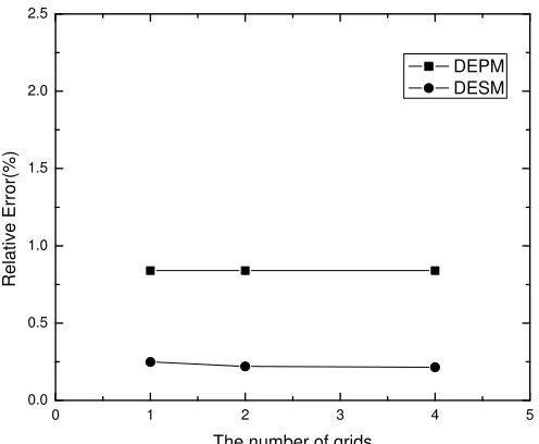
Figure 3.5. The relative error of estimations reported by DEPM and DESM using data set 1.
experiments. Our experiments are designed with two objectives in mind. First, we verify the
proposed methods, DEPM and DESM, are able to report highly accurate answers. Second,
we assess the two methods DEPM and DESM for their energy consumption.
To evaluate the two algorithms we proposed, we need the real data set to validate the
accuracy of DESM and DEPM. We use 20 TelosB sensors to sense and collect the intensity
of light as the testing data set. To prolong the lifetime of sensor network is our motivation
to propose these two algorithms, so we also test and analysis the energy consumption of each
algorithm.
3.3.1 Estimation accuracy
In this section, we report the results of DEPM and DESM and assess the accuracy of
the data estimates reported by the proposed methods. The average relative error is used as
the metric to measure the accuracy. We conducted the experiments with the three data sets
0 1 2 3 4 5 0.0 0.5 1.0 1.5 2.0 2.5 R e la ti ve E rr o r( % )
The number of grids
[image:46.612.184.430.104.314.2]DEPM DESM
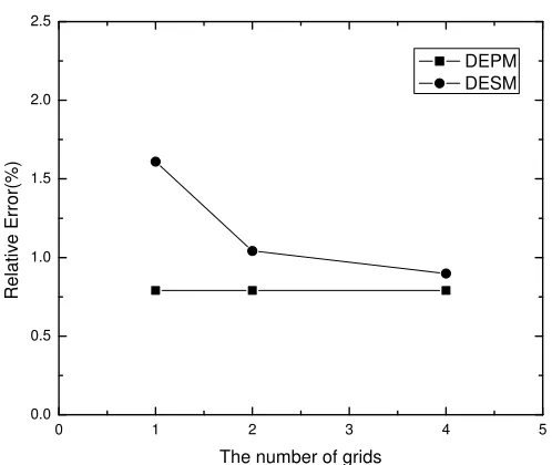
Figure 3.6. The relative error of estimations reported by DEPM and DESM using data set 2.
0 1 2 3 4 5
0.0 0.5 1.0 1.5 2.0 2.5 R e la ti ve E rr o r( % )
The number of grids
DEPM DESM
[image:46.612.182.431.431.641.2]As is shown in Figures 4.4, 4.5, and 4.6, with the number of grids increases, the relative
error of answers reported by DESM goes down. This is because the more the number of
grids is, the less the number of sensors in each grid, while the stronger the space locality of
sensors in one grid has. We could also see that DESM is more accurate for data set 1 but
gets worse for the data sets 2 and 3. The reason is that the light intensity values of data set
1 are stable while vary in the data set 2 and 3.
The accuracy of DEPM method has no relationship with the number of grids as shown
in Figures 4.4, 4.5 and 4.6. DEPM outperforms DESM on data set 2 and 3, but performs
worse on data set 1. Furthermore, obviously DEPM is not affected by different data sets. It
can keep good and stable quality on all three data sets.
3.3.2 Energy consumption
Table 3.2. System Parameters and Setting.
Parameter Setting
Number of sensor nodes 20
Message size 8 bytes
Transmission distance 50m
Energy Cost for Sending a Message 19.2uJ
Energy Cost for Receiving a Message 3.2uJ Energy Cost for Sensing a Light Intensity 100nJ
Energy Cost in Sleeping Mode 0.016mW
Initial Energy Budget at Each Sensor Node 1J
In this section, we assess the energy consumption. We use the energy model in [52] as
presented in Table 3.2. For the DESM and DEPM methods, one execution round is set to 10
minutes. For DESM, all the sensors collect data in the first two rounds of every two hours
considered as the history data. After the history data collecting phase, in each round one
node with the most remained energy works as an active node in every grid, and others go to
sleep in the rest time. For DEPM, in each round two nodes with the most remained energy
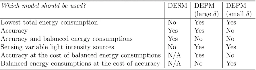
Table 3.3. Model Selection Guideline.
Which model should be used? DESM DEPM DEPM
(large δ) (small δ)
Lowest total energy consumption No Yes Yes
Accuracy Yes Yes No
Accuracy and balanced energy consumptions Yes No No
Sensing variable light intensity sources No Yes Yes
Accuracy at the cost of balanced energy consumptions N/A Yes No Balanced energy consumptions at the cost of accuracy N/A No Yes
We compare the proposed models with a naive model where all the sensors are set active.
As shown in Figure 4.8, the average energy consumption of both DEPM and DESM is much
less than that of the naive model. After running about 10 rounds, the accumulative average
energy consumption of DEPM is about 50% of that of the naive model. So DESM and DEPM
can prolong network lifetime effectively. DEPM is more effective than DESM, because DESM
has the collecting history data phase, consuming more energy. DESM-1 (DESM-2, DESM-4)
represents the DESM method with one grid (2 grids, 4 grids correspondingly) in the WSN.
From Figure 4.8, we can see that the more grids for DESM, the more energy consumption.
The reason is that each grid has an active sensor in DESM. The more number of grids means
the more sensors are set to active in the same time, hence the amount of energy consumed
is more.
We show the remained energy of DEPM with different constraints in Figure 3.9. It
is defined as the coefficient of variation of all the nodes’ remained energy. The average
energy consumption of all the nodes is almost half of initial energy. When we use larger δ,
the estimation accuracy is better, but it makes some nodes impossible to be active, so the
balance of energy consumptions is worse.
Neither DESM nor DEPM is a perfect method in all situations. Table 3.3 provides a
guide for choosing the proper estimation model in different situations. For instance, if users
prefer high accuracy, it is better to choose DESM or DEPM with large δ. If users expect
0 2 4 6 8 10 12 14 16 18 20 22 24 0 100 200 300 400 500 Naive Method DESM-1 DESM-2 DESM-4 DEPM A ccu m u la ti ve A ve ra g e E n e rg y C o n su m p ti o n (m Jo u le ) Round
Figure 3.8. The energy consumptions of different models.
0.00 0.01 0.02 0.03 0.04 0.05 0 1 2 3 4 5 6 7 delta
Remained Energy Balance Relative Error
[image:49.612.181.418.443.651.2]Chapter 4
IN-NETWORK HISTORICAL DATA STORAGE AND QUERY PROCESSING
In this chapter, we propose a scheme, HDQP, to store historical data locally on sensor
nodes and process historical data queries efficiently by using distributed index.
4.1 Historical Data Storage
Since a sensor node’s memory capacity is limited, we have to fully utilize it to store
as many data as possible. The administrator of the sensor network can specify the
at-tributes which need to be stored locally according to users’ requirements. Suppose there
are n attributes (A1, A2,· · · , An) need to be saved, and the sensor node senses the values
V1, V2,· · · , Vn of A1, A2,· · · , An respectively at sensing intervals. For each sensing interval,
a record with the format (T,V1, V2,· · · , Vn) (where T is a time-stamp) is written to the
flash memory. However, if the sensing interval is very short such as 5 seconds, the flash
memory will be full filled quickly. Then the rest of coming sensing data cannot be stored.
To avoid this happen, whenever the flash memory is occupied more than 80%, a
weight-reducing process is trigged. One record of every two consecutive records is erased. This
weight-reducing process can make at least half of memory space available again. Applying
the weight-reducing process repeatedly causes partial historical data lost. However, as we
mentioned in Chapter 1, even though the flash memory capacity is small, it still can store
5 to 10 values per hour for each attribute. Consequently, the historical data stored in the
flash memory can reflect the changing trend of each sensing attribute.
Each sensor node needs to calculate the maximum, minimum, and average for each
attribute periodically. The administrator specifies an update interval which is much greater