http://dx.doi.org/10.4236/jamp.2014.211112
Alternative Approaches of Convolution
within Network Calculus
Ulrich Klehmet, Rüdiger Berndt
Computer Networks and Communication Systems Friedrich-Alexander-Universität, Erlangen, Germany Email: [email protected], [email protected]
Received July 2014
Abstract
Network Calculus is a powerful mathematical theory for the performance evaluation of communi-cation systems; among others it allows to determine worst-case performance measures. This is why it is often used to appoint Quality of Service guarantees in packet-switched systems like the internet. The main mathematical operation within this deterministic queuing theory is the min- plus convolution of two functions. For example the convolution of the arrival and service curve of a system which reflects the data’s departure. Considering Quality of Service measures and per-formance evaluation, the convolution operation plays a considerable important role, similar to classical system theory. Up to the present day, in many cases it is not practical and simple to per-form this operation. In this article we describe approaches to simplify the min-plus convolution and, accordingly, facilitate the corresponding calculations.
Keywords
Network Calculus, Min-Plus Convolution, Algebraic Laws, Convex Analysis
1. Introduction
Timeliness plays an important role regarding systems with real time requirements. This Quality of Service (QoS) requirement can be found in many kinds of embedded systems which permanently exchange data with their en-vironment; like safety-critical automotive systems or real time networks. Since knowledge of mean values is not sufficient, analytical performance evaluation of such systems cannot be based on stochastic modeling as applied in traditional queuing theory. For these systems worst-case performance parameters like maximum delay of ser-vice times are required. In order to specify guarantees of performance figures—in terms of bounding values which are valid in any case—a mathematical tool Network Calculus (NC) as a novel system theory for determi-nistic queuing theory has been developed [1].
The development of this theory has been started by Cruz [2] [3] on the
(
σ ρ
,
)
traffic description and his calculus for network delay. Further steps towards NC were taken by the work of Parekh and Gallagher [4] to determine the service curve of Generalized Processor Sharing (GPS) schedulers. The NC framework has been successfully applied for the analysis and dimensioning in various domains, including industrial automation net-works [5] or automotive communications bus systems [6].subsequent Section 3 demonstrates the difficulties of convolution calculation and describes possible solution approaches. Finally, Section 4 draws a conclusion and indicates future steps.
2. Basic Modeling Elements of Network Calculus
The most important modeling elements of NC are the arrival curve (denoted by
α
in the figures) and the ser-vice curve (denoted byβ
in the figures) together with the min-plus convolution. The arrival and the service curve are the basis for the computation of maximum deterministic boundary values like backlog and delay bounds [1].Definition 1 (Arrival curve) Let
α
( )
t
be a non-negative, non-decreasing function. Flow F with input( )
x t
at time t is constrained by or has arrival curveα
( )
t
iffx t
( ) ( )
−
x s
≤
α
(
t s
−
)
for all t≥ ≥s 0. Flow F is also calledα
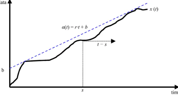
-smooth.Example 1 A commonly used arrival curve is the token bucket constraint:
( )
,
: 0 0 : 0
r b
b rt t
t
t
α = + >
≤
[image:2.595.164.463.544.706.2] (1)
Figure 1 shows an arrival curve which represents an upper limit for a given traffic flow
x t
( )
with an aver-age rate r and an instantaneous burst b. Therefore:( ) ( )
r b,(
)
x t
−
x s
≤
α
t s
−
. For ∆ = −t: t s and ∆ →t 0:( ) ( )
{
}
{
}
0
lim lim
t→s x t −x s ≤∆ →t r⋅ ∆ +t b =b (2) Next the convolution operation, which plays the most important role in Network Calculus will be defined. Definition 2 (Min-plus convolution) Let
f t
( )
andg t
( )
be non-negative, non-decreasing functions that are 0 for t≤0. A third function, calledmin-plus convolution is defined as(
)( )
{
( ) (
)
}
0infs tf g t f s g t s
≤ ≤
⊗ = + − (3)
On this basis we can characterize the arrival curve α
( )
t with respect to a givenx t
( )
as:x t
( ) (
≤ ⊗
x
α
)( )
t
In other words, arrival curves describe an upper bound to the input stream of a system. Considering the sys-tem’s output, we might be interested in service guarantees: like a minimum of outputy t
( )
, i.e. the amount of data that leaves the system. The following definition deals with this problem.Definition 3 (Service curve) Let a system S with input flow
x t
( )
and output flowy t
( )
be given. The system provides a (minimum) service curveβ
( )
t
to the flow, iffβ
( )
t
is a non-negative, non-decreasing function withβ
( )
0
=
0
and ify t
( )
is lower bounded by the convolution ofx t
( )
andβ
( )
t
, i.e.:( ) (
)( )
[image:3.595.172.445.533.699.2]y t
≥ ⊗
x
β
t
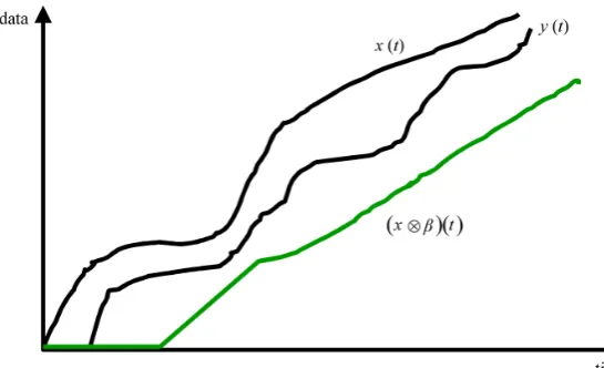
(4) Figure 2 shows(
x⊗β)( )
t =inf0≤ ≤s t{
x s( )
+β(
t−s)
}
as lower bound of outputy t
( )
and inputx t
( )
. Such service curves are functions of the time and describe the service of network elements like routers or sche-dulers in an abstract manner [7].Example 2 A commonly used service curve of practical applications is the rate-latency function:
( )
t R T,( )
t R t[
T]
: R max 0,{
t T}
β =β = ⋅ − + = ⋅ −
(5) This function reflects a service element which offers a minimum service of rate R after a worst-case latency of T. Since we want to analyze the worst-case performance, it is possible to abstractly model the complex in-ternal behavior of the node by just describing the worst-case service using this curve. This is very important in practical utilization.
In Figure 4, the (green) line depicts the rate-latency service curve with rate R and latency T.
Consider a system with input flow
x t
( )
, arrival curveα
( )
t
, output flowy t
( )
and service curveβ
( )
t
. According to [1] the following three bounds can be derrived:• Backlog Bound
v
:( )
( ) ( )
sups 0{
( )
( )
}
v t =x t −y t ≤ ≥ α s −β s• Delay Bound d in case of FIFO service:
( )
(
)
{
}
{
}
0 inf :
sups
d≤ ≥
τ α
s ≤β
s+τ
• Output Bound
α
∗( )
t :( )
t : sups 0{
(
t s)
( )
s}
α∗ α β α β
≥
= = + −
Remark:
The complete backlog
v t
( ) ( ) ( )
=
x t
−
y t
at time t within a system is also called unfinished work or buffer( )
t
. The expression inf{
τ α:( )
s ≤β(
s+τ)
}
is called virtual delay: the minimal time distance which is ne-cessary for inputx
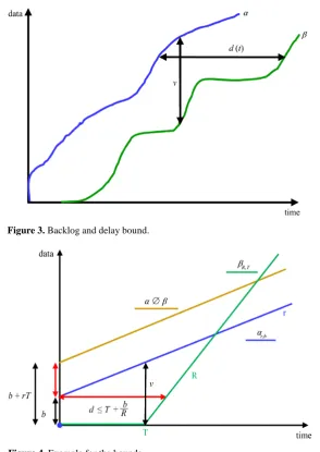
for being served to output. Thus, the backlog and delay bound are the maximal vertical and horizontal deviation between arrival and service curve. Figure 3 depicts d andv
for a given arrival- and service curve.Example 3 Let a system with a token bucket-smooth input and rate-latency service be given, thus:
( ) ( )
r b,(
)
x t
−
x s
≤
α
t s
−
and
( )
infs t{
( )
R T,(
)
}
y t ≥ ≤ x s +β t−s .
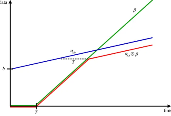
Based on the three bounds above we can calculate the delay bound as d T b R
≤ + , the output bound as
( ) (
t r t T)
bα
∗ = + +, and the backlog bound as v= +b rT. Figure 4 shows these results.
3. Difficulties of the Convolution Operation
Within the Network Calculus (NC) theory, the convolution operation of so-called min-plus algebra is considered the most essential operation. This is because—based on the arrival- and service curve—it computes the depar-ture of a network element, therefore it is the main instrument of analytical performance evaluation. For example in [1], this operation is carried out “by hand” using pure analytical calculation.
Take Example 3 for which αr b, ⊗βR T, as the lower bound for output y y: ≥αr b, ⊗βR T, needs to be com-puted.
3.1. Analytical Computation of Convolution Operator
⊗ [image:4.595.166.461.299.715.2]a) 0≤ ≤t T:
[image:4.595.171.455.525.704.2]Figure 3. Backlog and delay bound.
(
r b, R T,)
( )
inf{
r b,(
)
[
]
}
inf{
r b,(
)
0}
r b,( )
0 0 0s t s t
t t s R s T t s
α
β
α
+α
α
≤ ≤
⊗ = − + − = − + = + =
b) t>T:
(
)
( )
(
)
[
]
{
}
(
)
[
]
{
}
{
(
)
[
]
}
{
(
)
[
]
}
(
)
{
}
{
(
)
(
)
}
{
(
)
}
(
)
{
}
{
{
(
)
}
}
{
(
)
}
(
)
{
}
{
(
)
}
{
(
)
}
(
)
{
}
{
(
)
}
, ,
,
, , ,
inf
inf inf inf
inf 0 inf 0
inf r b R T
r b s t
r b r b r b
s T T s t s t
s T T s t
T s t t
t s R s T
t s R s T t s R s T t s R s T
b r t s b r t s R s T R t T
b r t T b rt RT R r s R t T
b r t T b r t T R t T
b r t T R t T
α β
α
α α α
+ ≤
+ + +
≤ ≤ ≤ =
≤ < <
< <
+ +
⊗
= − + −
= − + − ∧ − + − ∧ − + −
= + − + ∧ + − + − ∧ + −
= + − ∧ + − + − ∧ −
= + − ∧ + − ∧ −
= + − ∧ − .
(6)
Here
A B
∧ =
min
{ }
A B
,
and convolution(
αr b, ⊗βR T,)
with result (6) is depicted in Figure 5.For the following convolution of two rate-latency service curves (concatenation) a similarly complex calcula-tion is required.
( ) 1 1, 2,2 min 1, 2,1 2
R T R T R R T T
β β
= ⊗β
=β
+ (7)As we can see from above, this analytical approach is cumbersome and error-prone. But, similar to convolu-tion of classical systems theory, the convoluconvolu-tion ⊗ is of great importance for NC theory. This is why we are looking for other more elegant methods to computation.
Next, two alternative approaches called Use of algebraic laws and Use of convex analysis will be introduced.
3.2. Use of Algebraic Laws
In the following, the NC-relevant functions Φ are defined as non-negative, non-decreasing, and passing through the origin:
( )
( )
( )
{
f : f t1 f t0 0 t1 t0,f 0 0}
Φ = ≥ ≥ ∀ ≥ = (8)
[image:5.595.172.454.510.701.2]Among others, the following algebraic properties for the set of functions Φ can be found in literature [1]
• Rule 1 (Commutativity of ⊗): f ⊗ = ⊗g g f
• Rule 2 (Associativity of ⊗):
(
f
⊗ ⊗ = ⊗ ⊗
g
)
h
f
(
g
h
)
• Rule 3 (Distributivity of ⊗ and ∧):
h
⊗
(
f
∧
g
) (
= ⊗
h
f
) (
∧ ⊗
h
g
)
• Rule 4 (Addition of a constant):
g
⊗
(
K
+
f
)
= +
K
(
g
⊗
f
)
∀ ≥
K
0
• Rule 5 (Concave functions passing through the origin):f
⊗ =
g
min
{ }
f g
,
• Rule 6 (Shifting of f to right):
(
f ⊗δT)( )
t = f t(
−T)
+ withδ
T( )
t
=
0
for t≤T and ∞ otherwise. Now, we only apply these algebraic rules to compute the convolution ⊗.We consider Example 3 in an even more general form:
(
)
, ,
r b K R T
α ⊗ +β with any constant K; let λ = ⋅r r t
(
)
( )(
)
( )(
)
( )(
(
)
)
( )(
)
(
)
( )(
(
)
)
( )(
)
(
)
( )(
)
(
)
( )(
(
)
)
( )(
(
)
)
(
)
{
}
, ,Rule1 Rule6 Rule4
, , , ,
Rule2 Rule5 Rule3
, , ,
Rule6 Rule4 Rule6
, , , ,
r b R T
R T r b T R r b T R r b
T R r b T R r b T R T r b
R T T r R T T r R T r T
K
K K K
K K K
K b K b K b
K b r t T R
α β
β α δ λ α δ λ α
δ λ α δ λ α δ λ δ α
β δ λ β δ λ β β
+ ⊗ + = + ⊗ = + ⊗ ⊗ = + ⊗ ⊗ = + ⊗ ⊗ = + ⊗ ∧ = + ⊗ ∧ ⊗ = + ∧ ⊗ + = + ∧ ⊗ + = + ∧ +
= + + − ∧
{
(
t T−)
+}
.(9)
Or take the concatenation example:
β β
=
R T1 1,⊗
β
R T2,2:(
)
(
)
( )(
( )
)
(
( )
)
( )(
)
(
( )
( )
)
( )
{
}
(
( )
( )
)
( ){
}
(
(
)
)
( )1 2 1 2
1 2 1 2 1 2
Rule6 Rule2
1 1 2 2 1 2 1 2
Rule5 Rule6
1 2 1 2 1 2 min , ,
min , min , .
T T T T
T T R R T T
R t T R t T R t t R t t R t R t t t
R R t t t R R t T T
β δ δ δ δ
δ δ β
+ +
+
= − ⊗ − = ⊗ ⊗ ⊗ = ⊗ ⊗ ⊗
= ⊗ ⊗ = − + =
(10)
3.3. Use of Convex Analysis
The next approach is based on the theory of convex analysis [8]. Similar considerations related to NC theory can be found at [9]. However, we go another way considering “incomplete” convex functions. In Rockafellar’s book [8] all necessary preconditions for the following definition and proofs of the next theorems can be found.
Definition 4 (Conjugate function) Let f be any closed convex function on Rn.
( )
: supt{
,( )
dom}
f∗ s = s t − f t t∈ f is called the conjugate of f or Fenchel-transform, with , s t∈Rn
,
⋅ ⋅
the inner product in Rn.Theorem 1 (Conjugate f**) The conjugate
f
∗∗ off
∗ is f :( )
sups{
,( )
dom}
f∗∗ t = s t − f∗ s s∈ f∗ . Theorem 2 (Convolution) Let f1,,fn be proper convex functions on
n
R . Then:
(
f1 fn)
f1 fn∗ ∗ ∗
⊗ ⊗ = + + .
Remark:
In case of the convex NC functions of Φ: Rn ≡R1. From Theorem 1 and 2 we get
(
f1 fn)
(
f1 fn)
∗
∗ ∗
⊗ ⊗ = + + .
Example:
Again the aim is the concatenation
β β
=
R T1 1,⊗
β
R T2,2 with( )
(
)
,
: 1, 2 0 :
i i
i i i
R T
i R t T t T i t
t T
β = − ≥ =
<
First of all, the conjugate of the rate-latency function βR T, i.e.
β
R T∗, needs to be determined. From defini-tion 4 we know that( )
s supt{
st( )
t t dom}
supt{
st R t(
T)
}
β∗ = −β ∈ β = − − (12)
So, we get:
Case 0 :s<
β
∗( )
s = ∞ Case 0 :s=β
∗( )
s =0( )
: 0and for Case 0 :
:
Ts s R
s s
s R
β∗ < ≤
> =
∞ >
( )
,( )
: 0
Altogether: : 0
: R T
s
s s Ts s R
s R
β∗ β∗
∞ < = = ≤ ≤ ∞ > (13)
Determination of
β
∗∗( )
t as conjugate ofβ
∗( )
s withs
∈
dom
β
∗:( )
{
( )
}
{
,( )
: 0
sup sup : 0
:
s s R T
s
t st s st Ts s R t
s R
β∗∗ β∗ β
∞ < = − = − ≤ ≤ = ∞ > (14)
This certainly confirms Theorem 1. Applying Theorem 2:
(
β1 β2)
β1 β2∗ ∗ ∗
⊗ = + and by applying Theorem 1:
(
β1⊗β2)
∗∗=(
β1⊗β2)
; here(
β
1∗+β
2∗)
∗. For the concatenation1 1, 2,2
R T R T
β
⊗
β
we obtain (let1 1
1 R T,
β β
=
and2 2
2 R T,
β
=
β
, T2>T1>0, R2>R1 >0)(
1 2) ( )
1( )
2( )
1 1 2 2(
1 2)
11 2 1
: 0 : 0 : 0
: 0 : 0 : 0
: : :
s s s
s s s T s s R T s s R T T s s R
s R s R s R
β β ∗ β∗ β∗
∞ < ∞ < ∞ <
⊗ = + = ≤ ≤ = ≤ ≤ = + ≤ ≤
∞ > ∞ > ∞ >
(15)
(
1 2)
( )
{
(
1 2)
11 : 0
sup : 0
: s
s
t st T T s s R
s R
β∗ β∗ ∗
∞ < ⇒ + = − + ≤ ≤ ∞ > (16)
But this is the same structure as in expression for
β
∗∗( )
t and therefore(
β1 β2)
( )
t βR T1,1 T2 βmin(R R1, 2),T1 T2∗
∗ ∗
+ +
[image:7.595.179.459.540.700.2]+ = = holds. Figure 6 depicts this operation.
In conclusion, the use of convex analysis seems to be a further approach to determine the min-plus convolu-tion operaconvolu-tion—at least in the context of convex funcconvolu-tions like the set of piecewise linear funcconvolu-tions where βR T, belongs.
Question:
How to deal with non-convex functions f ∈ Φ. Take Example 3 with input x=αr b, and service curve ,
R T
β . The min-plus convolution realizes a guaranteed lower bound for the output: y t
( )
≥(
αr b, ⊗βR T,)
( )
t .( )
,
: 0 But function
0 : 0
r b
rt b t
t
t
α = + >
=
is not convex because the ≤ relation in:
(
)
(
)
(
)
( )
( )
, 1 0 1 1 , 0 , 1
r b t t r b t r b t
α −λ +λ ≤ −λ α +λα for t0 =0, t1∈R and 0< <λ 1 is not fulfilled. Therefore Theorem 1 and 2 are not readily applicable.
However, in contrast to [9] other ways are possible. Here the following one is suggested: making functions convex by redefining their values at certain points, e.g. where unnatural discontinuities appear (e.g. t=0). For example, we change
α
r b,( )
t
toα
r b,( )
t
such thatα
r b,( )
t
is convex and still reflects the arrival curve feature well:( )
,
for
0
r b
t
rt b
t
α
= +
≥
(17)Now, αr b, is convex and the principles of convex analysis are applicable. Although αr b, ∉ Φ (since
( )
,
0
0
r b
α
≠
) it represents the important burst feature∆ = − →
t
:
(
t s
)
0
of the arrival curve αr b, (of formula 2):( ) ( )
{
}
0{
}
0 ,( )
0 ,( )
limt→s x t −x s ≤lim∆ →t r⋅ ∆ +t b =lim∆ →t αr b ∆ =t lim∆ →t αr b ∆ =t b. Since αr b, ≠αr b, the convolution of
(
)
{
}
, ,
r b R T b r t T
α
β
+⊗ = + −
differs from
α
r b,β
R T,{
b r t T(
)
}
{
R t T(
)
}
+ +
⊗ = + − ∧ − .
The expression
{
b r t T+(
−)
+}
is identical in both formulas. When considering rate-latency functions (c.f. Example 2) where an incoming input is served with minimal rate R after a maximal delay T , the output y is lower bounded not only by{
b r t T+(
−)
+}
but by min{
b r t T+(
−)
+,R t T(
−)
+}
Of course, in the long run for t→ ∞ the term{
b r t T+(
−)
+}
is the dominant one, as you can see in Figure 5.4. Conclusions
The most important operation within the Network calculus is the min-plus convolution. But the calculation of this fundamental operation still is complex and error-prone. For this reason we introduced other computation approaches to perform the convolution: here called Use of algebraic laws and Use of convex analysis. In order to apply the convex analysis we transform non-convex into convex functions (e.g. keeping the token-bucket arrival curve property) which is different, for example, from the approach of [9].
This article reflects work in progress and the presented examples ought to demonstrate these techniques. In future work we will continue to investigate the procedures of subsection 3.2 and 3.3 to answer the following questions: Can we extend the principles to some classes of non-convex functions or even to mixed classes of convex and non-convex functions? Which kinds of applications are suited considering algebraic laws and con-vex analysis? Are there even cases where a combination of both methods is beneficial? To all of these, we want to find answers in future work.
References
[2] Cruz, R. (1991) A Calculus for Network Delay, Part I: Network Elements in Isolation. IEEE Transactions on Informa-tion Theory, 37, 114-131.
[3] Cruz, R. (1991) A Calculus for Network Delay, Part Ii: Network Analysis. IEEE Transactions on Information Theory,
37, 132-141.
[4] Parekh, A.K. and Gallager, R.G. (1993) A Generalized Processor Sharing Approach to Flow Control in Integrated Ser-vice Networks: The Single-Node Case. IEEE/ACM Transactions on Networking, 1, 344-357.
http://dx.doi.org/10.1109/90.234856
[5] Kerschbaum, S., Hielscher, K., Klehmet, U. and German, R. (2012) Network Calculus: Application to an Industrial Automation Network. In: MMB and DFT 2012 Workshop Proceedings (16th GI/ITG Conference), Kaiserslautern, March 2012.
[6] Herpel, T., Hielscher, K., Klehmet, U. and German, R. (2009) Stochastic and Deterministic Performance Evaluation of Automotive CAN Communication. Computer Networks, 53, 1171-1185.
http://dx.doi.org/10.1016/j.comnet.2009.02.008
[7] Fidler, M. (2010) A Survey of Deterministic and Stochastic Service Curve Models in the Network Calculus. IEEE Communications Surveys & Tutorials, 12, 59-86.
[8] Rockafellar, R.T. (1970) Convex Analysis. Princeton University Press.