Optimal Guaranteed Cost Control for Exponential Stability of Nonlinear System with Mixed Time-Varying Delays via Feedback Control

(1)

Optimal Guaranteed Cost Control for Exponential

Stability of Nonlinear System with Mixed

Time-Varying Delays via Feedback Control

Nuchira Khongja, Thongchai Botmart

Abstract—The problem of optimal guaranteed cost control for exponential stability of nonlinear system with mixed time-varying delays via feedback control is considered. The mixed time-varying delays consisting of both discrete and distributed delays are considered without assuming the differentiability of the time-varying delays. Based on an improved Lyapunov-Krasovskii functional with triple integral terms and employing Newton-Leibniz formula, Jensen’s inequality and reciprocal convex combination technique, new delay-dependent sufficient conditions for the existence of guaranteed cost feedback control for the system are given in terms of linear matrix inequalities (LMIs), which can be checked numerically by using the effective LMI toolbox in MATLAB. Finally, a numerical example is given to illustrate the effectiveness and improve over some existing results in the literature.

Index Terms—exponential stability analysis, nonlinear sys-tem, guaranteed cost control, feedback control, discrete and distributed time-varying delays

I. INTRODUCTION

I

N the scope of functional differential equations, stability and control problem has been the subject of investigable research attention. In most control engineering practice, it is always desirable to design a control system which is not only stabilizable but also guarantees an adequate level of performance. The guaranteed cost control was first put forward by Chang and Peng [5] and introduced by a lot of au-thors, which different design approaches have been proposed for systems with delay [11-14]. In [15], author designed state feedback guaranteed cost control of nonlinear systems with time-varying delay. By applying Lyapunov-Krasovskii functional method and linear matrix inequality technique, new delay-dependent sufficient conditions for designing the state feedback guaranteed cost control are derived. Optimal cost controller for linear system with mixed time-varying delays state and control has been considered in [18]. By improving Lyapunov-Krasovskii functionals with Newton-Leibniz formula, the sufficient conditions for the existence

Manuscript received December 7, 2017; revised January 29, 2018. The first author was supported by Research Publication Scholarship Fiscal Year of 2018, Graduate School of Khon Kaen University and Department of Mathematics, Faculty of Science, Khon Kaen University. The second author was supported by the National Research Council of Thailand and Faculty of Science, Khon Kaen University 2018 and the Thailand Research Fund (TRF), the Office of the Higher Education Commission (OHEC) (grant number : MRG6080239).

Nuchira Khongja is with the Department of Mathematics, Faculty of Science, Khon Kaen University, Khon Kaen 40002, Thailand. E-mail : [email protected].

Thongchai Botmart is with the Department of Mathematics, Faculty of Science, Khon Kaen University, Khon Kaen 40002, Thailand. E-mail : [email protected].

Correspondence should be addressed to Thongchai Botmart, [email protected].

of an optimal cost state feedback control for the system have been derived in term of LMIs.

Time-delay systems have actually been studied by several researchers. This may be the new emerging applications in engineering (such as network controlled systems) com-pounded with new theoretical results, that allowed one to solve some open problems (decoupling problems, stabiliza-tion, robustness, H∞ control, etc.) and less conservative

results. Absolutely, applications motivate the need of theory, which in return makes the control applications feasible.

Stability criteria for time-delay systems can be divided into two types: delay-dependent and delay-independent. Delay-dependent stability criteria are concerned with the size of the delay and usually provide a maximal delay size. On the other hand, delay-independent stability criteria tend to be more conservative, especially for small size delay, such criteria do not give any information on the size of the delay. There are many different methods given to deal with the stability problem. Among the well-known Lyapunov stability method, the Lyapunov functional is a powerful tool for stability analysis of time delay systems. Delay-dependent stability criteria for these systems are established in terms of linear matrix inequalities (LMIs).

In this research, we have considered the optimal guaran-teed cost control problem for a class of nonlinear system with mixed time-varying delays. The mixed time-varying delays consisting of both discrete and distributed delays are considered without assuming the differentiability of the time-varying delays. Based on an improved Lyapunov-Krasovskii functional with triple integral terms and employing Jensen’s inequality, Newton-Leibniz formula and reciprocal convex combination technique. A performance measure for the sys-tem is considered by a quadratic cost function. The feedback stabilizing controllers are designed to satisfy with exponen-tial stability. We give sufficient conditions for existence of the feedback guaranteed cost control in terms of LMIs, which can be determined by utilizing MATLABs LMI control toolbox. A numerical example is presented to show the effectiveness of the proposed method.

II. PRELIMINARIES

Notations

The following notation will be used in this paper : R+

denotes the set of all real nonnegative numbers;Rn denotes

the n−dimensional space and k · k denotes the Euclidean vector norm; An×m denotes the space of all matrices of

(n×m)-dimensions;AT denotes the transpose of matrixA;

(2)

λ(A) denotes the set of all eigenvalues of A; λmin(A) =

min{Reλ;λ ∈ λ(A)}; λmax(A) = max{Reλ;λ ∈ λ(A)};

xt= {x(t+s) : s ∈[−h,0]}; ||xt|| = sups∈[−h,0]||x(t+

s)||;C([0, t],_Rn₎_{denotes the set of all}

Rn-valued continuous

functions on[0, t];L2([0, t],Rm)denotes the set of allRm

-valued sguare integrable functions on [0, t]; Matrix A is called positive definite (A > 0) if xT_{Ax >} ₀ _{for all}

x ∈ Rn, x 6= 0; Matrix A is called semi-positive definite (A ≥ 0) if xTAx ≥ 0 for all x ∈ Rn; A > B means A−B >0. The symmetric term in a matrix is denoted by *.

Consider a nonlinear system with mixed time-varying delay of the form

˙

x(t) =Ax(t) +Bx(t−h1(t)) +C

Z t

t−d1(t)

x(s)ds

+f(t, x(t), x(t−h1(t)),

Z t

t−d1(t)

x(s)ds, u(t))

+U(t), (1)

U(t) =D1u(t) +D2u(t−h2(t)) +D3

Z t

t−d2(t)

u(s)ds,

x(t) =φ(t), t∈[−d3,0], d3=max{h1M, h2, d1, d2},

where x(t) ∈ Rn, u(t) ∈ Rm are the state and control,

respectively, the control u(·) ∈ L2([0, t],Rm), u(t) = Kx(t), K is constant matrix gain, φ(t) ∈ C([−d3,0],Rn)

is the initial function with the norm

||φ||=sup_t_∈_[₋_d₃_,_0]

q

||φ(t)||2₊_||_φ˙₍_t₎_||2_,

A, B, C, D1, D2, D3are given constant matrices with appro-priate dimensions, the delay functions hi(t), di(t), i = 1,2

satisfy the condition

0≤h1m≤h1(t)≤h1M, 0≤h2(t)≤h2,

0≤d1(t)≤d1, 0≤d2(t)≤d2,

η=h1M−h1m

and f(·) : R+ ×Rn ×Rn×Rn×Rm → Rn is a given

continuous function satisfying f(t,0,0,0,0) = 0,∀t ∈R+,

andf(t, x, y, z, u)satisfy Lipschitz condition with respect to

(x, y, z, u), such that ∃a, b, c, d >0 :

||f(t, x, y, z, u)|| ≤a||x||+b||y||+c||z||+d||u||. (2)

Define the following quadratic cost function of the asso-ciated system (1) as follows :

J =

Z ∞

0

L(t, x(t), x(t−h1(t)),

Z t

t−d1(t)

x(s)ds, u(t))dt,

(3)

where

L(·) ≤xT(t)Z1x(t) +xT(t−h1(t))Z2x(t−h1(t))

+

Z t

t−d1(t)

xT(s)ds

Z3

Z t

t−d1(t)

x(s)ds

+uT(t)Y1u(t),

Z1, Z2, Z3 ∈ Rn×n and Y1 ∈ Rm×m are positive definite

matrices.

The objective of this paper is to design a feedback con-trolleru(t) =Kx(t)and a finite number J∗ >0, such that the resulting closed-loop system

˙

x(t) = (A+D1K)x(t) +Bx(t−h1(t))

+C

Z t

t−d1(t)

x(s)ds+f(t, x(t), x(t−h1(t)),

Z t

t−d1(t)

x(s)ds, Kx(t)) +D2u(t−h2(t))

+D3

Z t

t−d2(t)

u(s)ds (4)

is exponentially stable and the valueJ(u)≤J∗_.

Definition 1. Givenα >0. The zero solution of closed-loob system (4) is α-exponentially stabilizable if there exists a positive number N > 0, such that every solution x(t, φ)

satisfies the following condition

||x(t, φ)|| ≤N e−αt||φ||, ∀t∈R+.

Definition 2. Consider the control system(1).If there exist a continuous stabilizing state feedback control lawu∗(t) = Kx(t)and a positive numberJ∗ _{such that the zero solution}

of the closed-loop system(4)is exponentially stable and the value (3) satisfies J(u∗)≤ J∗ then the cost value J∗ is a guaranteed cost value,u∗(t)is a guaranteed cost controller of the system.

Proposition 3. [9]. (Cauchy inequality) For any symmetric positive definite matrixN ∈Mn×n _and_{x, y}_∈

Rn we have

±2xTy≤xTN x+yTN−1y.

Proposition 4. [9]. (Schur complement lemma) Given con-stant symmetric matrices X, Y and Z with appropriate dimensions satisfying X = XT_{, Y} ₌ _YT _> ₀_{, then}

X+ZT_Y−1_{Z <}₀ _{if and only if}

X ZT

∗ −Y

<0 or

−Y Z

∗ X

<0.

Proposition 5. [17]. For any constant matrix Z =ZT >0

and positive numbersh,h¯ such that the following integrals are well defined, then

(i)−

Z t

t−h

x(s)TZx(s)ds

≤ −1

h

Z t

t−h

x(s)ds

T

Z

Z t

t−h

x(s)ds

.

(ii)−

Z −h

−¯h

Z t

t+s

x(τ)TZx(τ)dτ ds≤ −_¯ 2

h2₋_h2 ×

Z −h

−¯_h

Z t

t+s

x(τ)dτ ds

!T

Z

Z −h

−¯_h

Z t

t+s

x(τ)dτ ds

!

.

Proposition 6. [17]. Let f1, f2, ..., fN : Rm → R have

positive values in an open subset D of _Rm_{. Then, the}

reciprocally convex combination offi overD satifies

min{ri|ri>0,Piri=1}

X

i

1 ri

fi(t)

=X

i

fi(t) +maxgi,j(t)

X

i6=j

(3)

subject to

gi,j :Rm→R, gj,i(t) =gi,j(t),

fi(t) gi,j(t)

gi,j(t) fj(t)

≥0 .

III. MAIN RESULTS

The following theorem gives sufficient conditions for designing a guaranteed cost controller for system(1).

Theorem 7. Given α >0.Consider the system (1) and the cost function (3). If there exist symmetric positive definite matricesP, Q1, Q2, R1, R2, R3, R4, S1, T1, T2, W1, W2 andW3 satisfying the following LMIs

Φ =





Φ11 Φ12 Φ13 ∗ Φ22 Φ23

∗ ∗ Φ33



<0, (5)

then

u(t) =−1

2D

T

1P−

1_x₍_t₎_, _t_∈

R+ (6)

is a guaranteed cost controller and the guaranteed cost value is

J∗=λ2||φ||2_.

Moreover, the solutionx(t, φ)satisfies

||x(t, φ)|| ≤

r

λ2

λ1

e−αt||φ||, ∀t∈R+,

where

Φ11=



    

M1,1 M1,2 M1,3 M1,4 M1,5

∗ M2,2 0 0 0

∗ ∗ M3,3 0 0

∗ ∗ ∗ M4,4 0

∗ ∗ ∗ ∗ M5,5



    

,

Φ12=



    

0 M1,7 M1,8 M1,9 0

0 0 0 0 0

M5,6 M5,7 M5,8 0 0



    

,

Φ13=



    

M1,11 M1,12 M1,13 M1,14 0

0 0 0 0 0

0 0 0 M5,14 0



    

,

Φ22=



    

M6,6 0 0 0 0

∗ M7,7 M7,8 0 0

∗ ∗ M8,8 0 0

∗ ∗ ∗ M9,9 M9,10

∗ ∗ ∗ ∗ M10,10



    

,

Φ23=



    

0 0 0 0 0

0 0 0 M9,14 0

0 0 0 0 0



    

,

Φ33=



    

M11,11 0 0 0 0

∗ M12,12 0 0 0

∗ ∗ M13,13 0 0

∗ ∗ ∗ M14,14 M14,15

∗ ∗ ∗ ∗ M15,15



    

,

M1,1= [A+αI]P+P[A+αI]T+ (a+b+c+ 0.5d)I −D1D1T+dD1DT1 + 0.25D1Y1DT1 +Q1+Q2

+d2₁T2+ 3e2αh2D2S1DT2 + 2e 2αd2_D

3T1DT3 −e−2αh1m_R

1−e−2αh1MR2−2e−4αh1mW1 −2e−4αh1M_W

2−

2e−4αh1M₍_h

1M−h1m)

(h1M+h1m)

W3,

M1,2=P, M1,3= D1, M1,4= d22D1, M1,5= BP,

M1,7=e−2αh1mR1, M1,8= e−2αh1MR2, M1,9= CP,

M1,11=

2e−4αh1m

h1m

W1, M1,12=

2e−4αh1M

h1M

W2,

M1,13=

2e−4αh1M

(h1M+h1m)

W3, M1,14= P AT−0.5D1DT1,

M2,2= −(2aI+Z1)−1, M3,3= −2e2αh2S1,

M4,4= −4d22T1,

M5,5= −2e−2αh1MR3+e−2αh1M(R4+RT4),

M5,6=P, M5,7= e−2αh1MR3−e−2αh1MR4,

M5,8=e−2αh1MR3−e−2αh1MRT4, M5,14= P BT,

M6,6= −(2bI+Z2)−1,

M7,7= −e−2αh1mQ1−e−2αh1mR1−e−2αh1MR3,

M7,8=e−2αh1MRT4,

M8,8= −e−2αh1MQ2−e−2αh1MR2−e−2αh1MR3,

M9,9= −e−2αd1T2, M9,10= P, M9,14= P CT,

M10,10= −(2cI+Z3)−1, M11,11=

−2e−4αh1m

h2 1m

W1,

M12,12=

−2e−4αh1M

h2 1M

W2, M13,13=

−2e−4αh1M

(h2

1M−h21m)

W3,

M14,14=h21mR1+h21MR2+ (h1M−h1m)2R3+h21mW1

+h2₁_MW2+ (h1M−h1m)h1MW3

+ 3e2αh2_D

2S1DT2 + 2e 2αd2_D

3T1DT3

+ (a+b+c+ 0.5d)I−2P,

M14,15=h22D1, M15,15= −4h22S1,

λ1=λmin(P−1),

λ2=λmax(P−1) +h1mλmax(P−1Q1P−1)

+h1Mλmax(P−1Q2P−1)

+h3₁_mλmax(P−1R1P−1)

+h3₁_Mλmax(P−1R2P−1)

+ (h1M−h1m)3λmax(P−1R3P−1)

+1 4h

3

2λmax(P−1D1S1−1D

T

1P− 1₎

+1 4d

3

2λmax(P−1D1T1−1D

T

1P

−1₎

+d3₁λmax(P−1T2P−1)

+h3₁_mλmax(P−1W1P−1)

+h3₁_Mλmax(P−1W2P−1)

+ (h1M−h1m)h21Mλmax(P−1W3P−1).

(4)

V(t, xt) =

12

X

i=1

Vi(t, xt),

where

V1(·) =xT(t)Y x(t),

V2(·) =

Z t

t−h1m

e2α(s−t)xT(s)Y Q1Y x(s)ds,

V3(·) =

Z t

t−h1M

e2α(s−t)xT(s)Y Q2Y x(s)ds,

V4(·) =h1m

Z 0

−h1m

Z t

t+s

e2α(θ−t)x˙T(θ)Y R1Yx˙(θ)dθds,

V5(·) =h1M

Z 0

−h1M

Z t

t+s

V6(·) =η

Z −h1m

−h1M

Z t

t+s

V7(·) =h2

Z 0

−h2

Z t

t+s

e2α(θ−t)u˙T(θ)S₁−1u˙(θ)dθds,

V8(·) =d2

Z 0

−d2

Z t

t+s

e2α(θ−t)uT(θ)T₁−1u(θ)dθds,

V9(·) =d1

Z 0

−d1

Z t

t+s

e2α(θ−t)xT(θ)Y T2Y x(θ)dθds,

V10(·) =

Z 0

−h1m

Z 0

τ

Z t

t+s

e2α(θ+s−t)x˙T(θ)Y W1Yx˙(θ)×

dθdsdτ,

V11(·) =

Z 0

−h1M

Z 0

τ

Z t

t+s

dθdsdτ,

V12(·) =

Z −h1m −h1M

Z 0

τ

Z t

t+s

dθdsdτ.

It is easy to check that

λ1||x(t)||2≤V(t, xt)≤λ2||xt||2, ∀t≥0. (7)

Taking the derivative of Vi(t, xt) along the solution of the

system by using Newton-Leibniz formula, condition (2), Proposition 3, Proposition 5, Proposition 6, we have

˙

V(t, xt) + 2αV(t, xt)≤ξT(t) Πξ(t)−L(·) (8)

where

ξT(t) =

yT(t), yT(t−h1(t)), yT(t−h1m), yT(t−h1M),

Z t

t−d1(t)

yT(s)ds,

Z t

t−h1m

yT(τ)dτ,

Z t

t−h1M

yT(τ)dτ,

Z t−h1m

t−h1M

yT(τ)dτ,y˙T(t)

,

Π =





Π11 Π12 Π13 ∗ Π22 Π23

∗ ∗ Π33



<0, (9)

Π11=





N1,1 N1,2 N1,3 ∗ N2,2 N2,3 ∗ ∗ N3,3



,

Π12=





N1,4 N1,5 N1,6

N2,4 0 0

N3,4 0 0



,

Π13=





N1,7 N1,8 N1,9

0 0 N2,9

0 0 0



,

Π22=





N4,4 0 0

∗ N5,5 0 ∗ ∗ N6,6



,

Π23=





0 0 0

0 0 N5,9

0 0 0



,

Π33=





N7,7 0 0

∗ N8,8 0 ∗ ∗ N9,9



,

N1,1= [A+αI]P+P[A+αI]T + (a+b+c+ 0.5d)I −D1DT1 +dD1DT1 + 0.25D1Y1DT1 +Q1+Q2

+d2₁T2+ 3e2αh2D2S1D2T + 2e 2αd2_D

3T1D3T −e−2αh1m_R

1−e−2αh1MR2−2e−4αh1mW1 −2e−4αh1M_W

2−

2e−4αh1M₍_h

1M−h1m)

(h1M+h1m)

W3

+P(2aI+Z1)P+ 0.5e−2αh2D1S1−1D

T

1

+ 0.25d2₂D1T1−1D

T

1,

N1,2=BP, N1,3= e−2αh1mR1, N1,4= e−2αh1MR2,

N1,5=CP, N1,6=

2e−4αh1m

h1m

W1,

N1,7=

2e−4αh1M

h1M

W2, N1,8=

2e−4αh1M

(h1M+h1m)

W3,

N1,9=P AT −0.5D1D1T,

N2,2= −2e−2αh1MR3+e−2αh1M(R4+RT4)

+P(2bI+Z2)P,

N2,3=e−2αh1MR3−e−2αh1MR4,

N2,4=e−2αh1MR3−e−2αh1MRT4, N2,9= P BT,

N3,3= −e−2αh1mQ1−e−2αh1mR1−e−2αh1MR3,

N3,4=e−2αh1MRT4,

N4,4= −e−2αh1MQ2−e−2αh1MR2−e−2αh1MR3,

N5,5= −e−2αd1T2+P(2cI+Z3)P, N5,9= P CT,

N6,6=

−2e−4αh1m

h2 1m

W1, N7,7=

−2e−4αh1M

h2 1M

W2,

N8,8=

−2e−4αh1M

(h2

1M−h21m)

W3,

N9,9=h21mR1+h21MR2+ (h1M−h1m)2R3+h21mW1

+h2₁_MW2+ (h1M−h1m)h1MW3

+ 3e2αh2_D

2S1D2T+ 2e2αd2D3T1D3T

+ (a+b+c+ 0.5d)I−2P+ 0.25h2₂D1S1−1D

T

(5)

Using Proposition 4 (Schur complement lemma), condition

(5)is equivalent to the conditionΠ<0. Thus, from(5)−(9)

,we obtain

˙

V(t, xt) + 2αV(t, xt)≤ −L(·), ∀t∈R+. (10)

Since L(·)>0, we have

˙

V(t, xt)≤ −2αV(t, xt), ∀t∈R+. (11)

Integrating both sides of(11)from0 tot, we obtain

V(t, xt)≤V(0, x0)e−2αt, ∀t∈R+.

Furthermore, taking condition(7)into account, we have

λ1||x(t, φ)||2≤V(t, xt)≤V(0, x0)e−2αt≤λ2e−2αt||φ||2, then

||x(t, φ)|| ≤

r

λ2

λ1

e−αt||φ||, ∀t≥0,

which implies the exponential stability of the closed-loop system(4). To find the upper bound of the cost function(3), we consider the derived condition(10)andV(t, xt)>0,we

have

˙

V(t, xt)≤ −L(·), ∀t∈R+. (12)

Integrating both sides of(12)from0 tot, we obtain

Z t

0

L(·)dt≤V(0, x0)−V(t, xt)≤V(0, x0), ∀t∈R+,

because ofV(t, xt)>0. Hence, letting t → ∞, we finally

obtain that

J =

Z ∞

0

L(·)dt≤V(0, x0)≤λ2||φ||2=J∗.

This completes the proof of the theorem.

IV. NUMERICALEXAMPLES

In this section, we now provide an example to show the effectiveness of the result in Theorem 7.

Example.1Consider a nonlinear system and mixed time-varying delay using feedback control with the following :

˙

x(t) =Ax(t) +Bx(t−h1(t)) +C

Z t

t−d1(t)

x(s)ds

+f(t, x(t), x(t−h1(t)),

Z t

t−d1(t)

x(s)ds, u(t))

+U(t), (1)

U(t) =D1u(t) +D2u(t−h2(t)) +D3

Z t

t−d2(t)

u(s)ds,

x(t) =φ(t), t∈[−d3,0], d3=max{h1M, h2, d1, d2}, where

A=

0 0 0 1

, B=

−2 −0.5 0 −1

,

C=

−0.2 0 0 −0.1

, D1=

2 0 0 3

,

D2=

0.1 0 0 0.1

, D3=

0.1 0 0 0.1

,

Z1=Z2=Z3=Y1=

0.1 0 0 0.1

,

a=b=c=d= 0.001, α= 0.01,

h2= 0.3, h1m= 0.1, h1M= 0.3,

d1= 0.03, d2= 0.02.

By using the LMI Toolbox in MATLAB, we obtain

P =

4.5599 −0.6159

−0.6159 3.8500

,

Q1=

3.8029 0.5375 0.5375 1.8969

,

Q2=

4.2538 0.4146 0.4146 1.0766

,

R1=

17.9365 −15.9555

−15.9555 48.7317

,

R2=

0.3552 −0.7884

−0.7884 2.3270

,

R3=

20.7980 −3.6989

−3.6989 18.9409

,

R4=

1.0501 −2.6087

−2.6087 7.6735

,

S1=

5.2109 −1.8802

−1.8802 12.7356

,

T1=

1.0972 −2.2022

−2.2022 6.1546

,

T2=

82.1632 −80.0082

−80.0082 205.1834

,

W1=

2.4264 −4.0157

−4.0157 12.5592

,

W2=

0.5094 −1.1200

−1.1200 3.3355

,

W3=

0.1800 −0.2595

−0.2595 0.7044

,

K=

−0.2241 −0.0359

−0.0538 −0.3982

,

and the feedback control is

u(t) =

−0.2241 −0.0359

−0.0538 −0.3982

x(t),

λ1= 0.2034, λ2= 0.4143.

We take the initial condition

φ(t) =

0.5sint 0.5cos t

,

||φ||= 1

and the guaranteed cost value is

J∗= 0.4143||φ||2_{= 0}_.₄₁₄₃_.

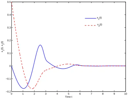
By Theorem 1, the system is exponentially stable and solu-tionx(t, φ(t))satisfies

(6)

0 1 2 3 4 5 6 7 8 9 10 −0.2

−0.1 0 0.1 0.2 0.3 0.4 0.5

Time t x1

(t), x

2

(t)

x₁(t)

x

[image:6.595.57.284.54.229.2]

2(t)

Fig. 1. The trajectoriesx1(t), andx2(t)of closed-loop system

V. CONCLUSION

In this paper, we have investigated the problem of optimal guaranteed cost control for exponential stability of nonlinear system with mixed time-varying delays via feedback control. The mixed time-varying delays consisting of both discrete and distributed delays are considered without assuming the differentiability of the time-varying delays. Based on an improved Lyapunov-Krasovskii functional with triple integral terms, new delay-dependent sufficient conditions for the existence of guaranteed cost feedback control for the system are given in terms of linear matrix inequalities (LMIs). A performance measure for the system is considered by a quadratic cost function. Finally, a numerical example is given to illustrate the effectiveness and improve over some existing results in the literature.

ACKNOWLEDGMENT

The authors thank anonymous reviewers for their valuable comments and suggestions.

REFERENCES

[1] B. T. Anh, N. K. Son and D. D. X. Thanh, “Stability Radii of Positive Linear Time-Delay Systems under Fractional Perturbations,”Systems & Control Letters,vol. 58, pp. 155-159, 2009.

[2] T. Botmart, P. Niamsup, and V. N. Phat, “Delay-Dependent Expo-nential Stabilization for Uncertain Linear Systems with Interval Non-Differentiable Time-Varying Delays,”Applied Mathematics and Com-putation,vol. 217, pp. 8236-8247, 2011.

[3] T. Botmart and W. Weera, “Guaranteed Cost Control for Exponential Synchronization of Cellular Neural Networks with Mixed Time-Varying Delays via Hybrid Feedback Control,”Abstract and Applied Analysis,

vol. 2013, Article ID 175796, 12 pages, 2013.

[4] J. Cao, J. Zhong and Y. Hu, “Novel Delay-Dependent Stability Conditions for MIMO Networked Control Systems with Nonlinear Perturbation,”Applied Mathematics and Computation, vol. 197, pp. 797-809, 2008.

[5] S. S. L. Chang and S. S. L. Peng, “Adaptive Guaranteed Cost Control of Systems with Uncertain Parameters,” Institute of Electrical and Electronics Engineers, Transactions on Automatic Control,vol. 17, pp. 474-483, 1972.

[6] W. H. Chen, Z. H. Guan and X. Lu, “Delay-Dependent Output Feedback Guaranteed Cost Control for Uncertain Time-Delay Systems,” Auto-matica. A Journal of IFAC, the International Federation of Automatic Control,vol. 40, pp. 1263-1268, 2004.

[7] E. N. Chukwu, Stability and Time-Optimal Control of Hereditary Systems,Boston: Academic Press, 1992.

[8] E. Fridman and S. I. Niculescu, “On Complete LyapunovKrasovskii Functional Techniques for Uncertain Systems with Fast-Varying De-lays,”International Journal of Robust and Nonlinear Control,vol. 18, pp. 364-374, 2008.

[9] K. Gu, V. L. Kharitonov and J. Chen,Stability of Time-Delay System,

Boston, Mass, USA: Birkhaauser, 2003.

[10] Y. He, Q. Wang, C. Lin and M. Wu, “Delay-Range-Dependent Stability for Systems with Time-Varying Delay,”Automatica. A Journal of IFAC, the International Federation of Automatic Control,vol. 43, pp. 371-376, 2007.

[11] T. H. Lee, D. H. Ji, J. H. Park and H. Y. Jung, “Decentralized Guaranteed Cost Dynamic Control for Synchronization of a Complex Dynamical Network with Randomly Switching Topology,” Applied Mathematics and Computation,vol. 219, pp. 996-1010, 2012. [12] T. H. Lee, J. H. Park, D. H. Ji, O. M. Kwon and S. M. Lee,

“Guar-anteed Cost Synchronization of a Complex Dynamical Network via Dynamic Feedback Control,”Applied Mathematics and Computation,

vol. 218, pp. 6469-6481, 2012.

[13] Y. S. Lee, Y. S. Moon and W. H. Kwon, “Delay-Dependent Guaranteed Cost Control for State Delayed Systems,”Proceeding of the American Control Conference, Arlington,pp. 3376-3381, 2011.

[14] S. O. Moheimani and I. R. Petersen, “Optimal Quadratic Guaranteed Cost Control of a Class of Uncertain Time-Delay Systems,” IEE Proceedings-Control Theory and Applications,vol. 144, pp. 183-188, 1997.

[15] P. Niamsup and V. N. Phat, “State Feedback Guaranteed Cost Con-troller for Nonlinear Time-Varying Delay Systems,”Vietnam Journal of Mathematics,vol. 43, pp. 215-228, 2015.

[16] N. K. Son and P. H. A. Ngoc, “Stability Radii of Linear Functional Differential Equations,”Vietnam Journal of Mathematics,vol. 29, pp. 85-89, 2001.

[17] N. T. Thanh and V. N. Phat, “H∞Control for Nonlinear Systems with

Interval Non-Differentiable Time-Varying Delay,”European Journal of Control,vol. 19, pp. 190-198, 2013.

[18] M. V. Thuan and V. N. Phat, “Optimal Guaranteed Cost Control of Linear Systems with Mixed Interval Time-Varying Delayed State and Control,”Journal of Optimization Theory and Applications, vol. 152, pp. 394-412, 2012.

[19] W. Zhang, X. S. Cai and Z. Z. Han, “Robust Stability Criteria for Sys-tems with Interval Time-Varying Delay and Nonlinear Perturbations,”