Analysing gCSP models using runtime and model analysis algorithms

(1)

University of Twente

EEMCS / Electrical Engineering

Control Engineering

Analysing gCSP models using runtime

and model analysis algorithms

Maarten Bezemer

MSc report

Supervisors: prof.dr.ir. J. van Amerongen

dr.ir. J.F. Broenink ir. M.A. Groothuis

November 2008

(2)

(3)

Summary

Nowadays the amount of embedded systems is getting bigger and bigger. The systems themselves also become more complex. To aid developers of embedded systems a formal language called Communicating Sequential Processes (CSP) was designed.

At the Control Engineering (CE) group a graphical tool called gCSP is developed to create CSP models. This tool allows for code generation. The generated code can be compiled with the Communicating Threads (CT) library into an executable. Users of gCSP tend to create a separate process for each task. From the model point of view this is excellent, but from a software point of view this consumes too many resources.

First of all a new gCSP file format is created, such that an algorithm is able to read model infor-mation without too much effort. Next algorithms are designed and implemented, which perform analysis on models using different techniques.

This assignment results into two analysis tools, which are able to perform an analysis of gCSP models. The first tool is a runtime analyser and uses the compiled executable to get information of the order in which the processes are running. The second tool is a model analyser which directly analyses a gCSP model. It creates a dependency graph and will try to group processes which are related to each other, resulting in a schedule for multi-core target systems. For single-core target systems the results can be used to recreate the model with a few bigger processes.

Both tools are tested to see whether they both are functional and usable. Functional tests are executed using a simple model to be able to manually check the analysis results with the expected outcome. The usability tests perform tests using a series of models and interpret the outcome of the analysers.

(4)

Samenvatting

Tegenwoordig wordt het aantal ‘embedded’ systemen groter en groter. De systemen zelf wor-den daarbij ook nog eens complexer. Om ontwikkelaars hierbij te helpen is er een formele taal ontwikkeld genaamd ‘Communicating Sequential Processes’ (CSP).

De Control Engineering (CE) vakgroep heeft een tool genaamd gCSP ontwikkeld om CSP model-len te maken. Met deze tool is het mogelijk om broncode te genereren. Deze broncode kan worden gecompileerd samen met de ‘Communicating Threads’ bibliotheek tot een uitvoerbare applicatie. Gebruikers van gCSP hebben de neiging om een proces te maken voor elke afzonderlijk taak. Vanuit het oogpunt van het modelleren is dit uitstekend, maar vanuit het oogpunt van de software gebruikt het te veel resources.

Ten eerste is een nieuw gCSP formaat nodig, zodat een algoritme in staat is om de model infor-matie zonder te veel moeite te kunnen lezen. Vervolgens zijn er algoritmes ontwikkeld die met verschillende technieken analyses op de modellen uitvoeren.

Het project heeft geresulteerd in twee tools waarmee analyses op gCSP modellen uitgevoerd kun-nen worden. De eerste tool is een runtime analyse tool die gebruikt maakt van de gecompileerde applicatie om informatie over de uitgevoerde volgorde van de processen te vinden. De tweede tool is een model analyse tool die direct het model analyseerd. Het bepaalt de afhankelijkheden en zal proberen de processen die samenhangen te groeperen, resulterend in een indeling voor multi-core systemen. Voor single-core systemen kunnen de resultaten gebruikt worden om van de kleine processen aan aantal grotere processen te maken.

Beide tools zijn getest om te bepalen of ze beide functioneel en bruikbaar zijn. Functionele testen zijn uitgevoerd met behulp van een simpel model, zodat het mogelijk is om handmatig de resulta-ten te controleren. De bruikbaarheidtesresulta-ten zijn gedaan met verscheidene modellen en de resultaresulta-ten hiervan zijn geïnterpreteerd.

(5)

1 Introduction

1.1 Context

More and more machines and consumer applications contain embedded systems to perform their main operations. Embedded systems are special purpose computers which are embedded into a machine or product. They are fed by signals from the outside world and use these signals to control the machine. Designing embedded systems becomes more and more complex since the requirements grow.

To aid developers with this complexness Hoare (1985) and Roscoe (1997) developed a formal lan-guage called Communicating Sequential Processes (CSP). It can be used to describe systems with several computational processes running at the same time, called concurrent systems. Embedded systems typically are such systems, so CSP is of great use for developers of embedded systems.

At the University of Twente, the Control Engineering group has created a tool to graphically design CSP models, called gCSP (Jovanovic et al., 2004). gCSP is able to generate code which can be executed on a PC or on a (real-time) hardware target. The generated code makes use of the Communicating Threads (CT) library (Hilderink et al., 1997), which provides a framework for the CSP language. The CSP application can be monitored in gCSP through an animation functionality (van der Steen, 2008). The complete overview is shown in Figure 1.1.

gCSP model

Code generation

CT library

Executable +

Animation gCSP Tool

Figure 1.1, Overview of the gCSP & CT framework

A number of undesired features are introduced by the current CSP implementation:

• The models tend to get extensive for large systems. This might result in sub-optimal models,

because the software designer is unable to think of all details.

• The control software designers tend to put every controlling part in a small process. This is

good in a design point of view, but in an executing point of view it results in a lot of wasted resources. To prevent wasting resources, the model ideally should be flattened into a single process without losing its desired functionality.

• The CT library is designed to run on a single-core target. The scheduler and all of its

processes run in the same software thread. Nowadays (computer) systems do not get much faster processors anymore. Instead the processors consist of multiple cores and gain higher speeds by allowing parallel execution of the threads. Distributed systems also make use of multiple codes, distributed over a networked system.

The first two points can be solved by aiding developers with the creation of the models. the last point is addressed by taking steps to make the CT library multi-core aware (Molanus, 2008; Veldhuijzen, 2008). In the future, the library is going to take advantage of these new developments. This project assumes the multi-core awareness of the library already.

1.2 Goals of the assignment

(10)

[image:10.595.188.383.144.247.2]

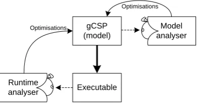
For both single and multi-core targets the results must also be usable to see how the model can be optimised in order to save resources. Two methods of analysis will be implemented as shown in Figure 1.2.

gCSP (model)

Executable

Optimisations

Model analyser

Runtime analyser

Optimisations

Figure 1.2, Overview of the locations of the analysers

The runtime analyser looks at the executing application, especially at its performance and be-haviour. Its results can be used to determine a static order of running processes. The model analyser looks at the models directly and schedules the processes on a number of available cores.

Both analysers should get different results due their different points of view. These results can be combined and used to make an optimised version of the model.

1.2.1 The runtime analyser

The runtime analyser should use runtime information to get a process order. In order to be able to get runtime information, the analyser should be able to connect to a running gCSP model. So it can retrieve information about the available processes. This information should be fed to an algorithm which will analyse the running model and produce chains of processes to show the running order of the process.

When the algorithm is designed and implemented in a tool, the results should be usable

• to get information in order to get a better understanding of the model

• to ideally provide enough information to optimise the model. For example to combine

several sequential processes into one larger process.

1.2.2 The model analyser

The model analyser should be able to analyse the model during design time. It loads a model and uses its information to create a dependency graph. This graph can be used to schedule the processes in such a way that a optimal schedule is obtained for a given target system.

In order to be able to read the model information, this information should be easily accessed. This is not the case in the current gCSP models, so a new format will be created. This format should be described by a meta-model. A meta-model is a model of a model, so the contents of the actual model are predefined. The new meta-model should be able to contain all required data for the analyser. It should provide functionality to store and load the model and it can function as a basis for an improved gCSP application.

At the end of the trajectory the tool implementing the model analysis algorithm should produce information

• which indicates how the processes are related to each other

• how the processes could be scheduled on the given target system consisting of at least one

core

(11)

1.3 Report outline

Before starting to describe the algorithms and their requirements, a background chapter explains the environment more extensively. Chapter 2 contains this background information. Chapter 3 describes the design of the runtime analyser, its algorithm, implementation and results. Chapter 4 and 5 describe the choices of input mechanisms for the new gCSP meta-model and the meta-model itself.

This information is required for the model analyser, which is described in Chapter 6.Like the run-time analyser chapter, this chapter also describes the design of the algorithm, the implementation and the analysis results. More information about the model analysis algorithms can be found in Appendices C and D.

(12)

2 Background

This chapter describes the background of the assignment. The first section contains information about related work, on which parts of the solutions are inspired. The next section describes the tools and workflow used at the CE group. Followed by a short description on the gCSP file format. The chapter ends with a section providing information about multi-core environments.

2.1 Related work

This section describes related work on scheduling models for usage on multiple processing units. Firstly Boillat and Kropf (1990) designed a distributed mapper algorithm that runs on the target system itself. It maps the processes in a optimal way, by starting to place the processes on the network. It measures the delays and calculates a quality factor. The processes, which have a bad influence on the quality factor, are remapped and the quality if determined again. This optimising analysis method is called post-game analysis. The used target system is a transputer network of which the communication delays and network connections differs depending on the nodes which need to communicate. Points of interest are:

• the algorithm to find a mapping such that the processes on a transputer only need

connec-tions to their neighbouring transputers. A transputers only can communicate to its bouring transputers, other transputers can be reached by finding a path using the neigh-bouring relations. This obviously is undesired, since it delays multiple other transputers as well.

• the optimisation for load balancing and communication minimisations, so the available

re-sources are optimally used.

• the fact that the mapping algorithm is designed to be distributed. This might save analysis

time for large transputer networks with a lot of possibilities.

Magott (1992) tried to solve the optimisation evaluation by using Petri nets. First a CSP model is converted to such a Petri net, which forms a kind of dependency graph, but still contains a complete description of the model. His research added time factors to these Petri nets and using these time factors he is able to optimise the analysed models.

Finally van Rijn (1990) describes an algorithm to parallelise model equations in his masters the-sis. He defined equation dependencies and used those to schedule the equations on a transputer network. Equations with a lot of dependencies form heaps, which are a kind of groups. These heaps should be kept together to minimise the communication costs. Furthermore, his scheduling algorithm tries to find a balanced load for the transputers, but keeping the critical path as short as possible.

This assignment mainly makes use of the work of van Rijn. Especially since the equations he tried to optimise could be compared to the CSP processes. His algorithms work without the need of the target system during analysis, although it is possible to run the algorithms on the target system as well if required. This is not the case for the work of Boillat and Kropf, their algorithm must be run on the target system, since the timing information needs to be measured. Their distributed analysis algorithm is not usable in this situation, since single-core target systems must be supported as well.

2.2 Tools and workflow

At the Control Engineering (CE) group a trajectory to design embedded software is developed (Broenink et al., 2007). Figure 2.1 shows this trajectory. The dashed box shows the steps in the trajectory where this assignment could be placed in.

(13)

Physical System Modelling

Verification by Simulation

Control Law Design

Embedded Control System Implementation

Realisation

Validation and Testing

Figure 2.1, Control software design trajectory

Short descriptions of the steps are:

• Physical System Modelling

A dynamic behaviour of the system is modelled. This can be done using bond graphs and 20-sim (Controllab Products, 2008).

• Control Law Design

The model containing the dynamic behaviour is converted into a set of control laws.

• Embedded Control System Implementation

The control laws are changed into (software) algorithms. For this task a graphical tool called gCSP (Jovanovic et al., 2004) is used.

• Realisation

The gCSP model is converted into an executable which can be run on a computer, ADSP, FPGA or ARM. CSP execution functionality is added by the CT library (Hilderink et al., 1997).

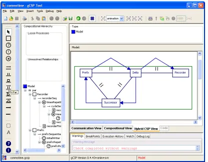
gCSP is a graphical tool to build models containing some sort of control algorithm, shown in Figure 2.2. More information on the CT library and the graphical modeling language can be found in (Hilderink, 2005) chapter 3.

In order to create an application from a gCSP model the Communicating Threads (CT) library is used as execution framework. This library defines the CSP constructions so they can be used by the application without the need of implementing them manually. The overview of the relations between gCSP, CT library and this assignment can be seen in Figure 1.2.

2.3 gCSP file format

When a model is drawn in gCSP, it can be stored in the Extensible Markup Language (XML) (World Wide Web Consortium, 2008) format. This is a well-defined format and very usable for the job.

However, by using XML one is free to choose how the data itself is stored within XML. gCSP chooses to store its memory directly into the XML format using the Java XML serialiser. This results in large files which are hard to read with an application other than gCSP. These files also get excessively large because the model objects have several copies of itself in the memory which all get stored separately.

Since this project is all about creating two tools (external applications) to analyse gCSP models this will be a problem. Hence the choice in the previous chapter to create a new meta-model, with a better and simpler defined structure.

2.4 Multi-core environments

(14)

[image:14.595.78.496.77.402.2]

Figure 2.2, gCSP user interface, showing parallel processes connected with channels

program which has its own task and is able to perform it without (much) need of other threads. Each thread could be executed by its own core, resulting in real parallel running software blocks.

It might be clear that this is speeding up the execution of applications greatly, which is a desired feature for control software as well. An example of control software that needs to run in parallel on a distributed system is the software for TUlip (3TU, 2008). It is a (soccer) robot which has multiple controllers connected to each other, in order to control the complete robot.

However, designing a (CSP) application for a multi-core system is tricky (Sputh et al., 2006) since the available processes should be scheduled into threads. When the processes are scheduled in a bad way the performance is not improving as much as possible and might even be dropping. So this project will assume the availability of a CT library with multi-core support and will present analysers which will help scheduling processes into threads which can be run on the available cores of the target system.

(15)

3 Runtime Analyser

This chapter describes the algorithms and the implementation of the ‘gCSP Runtime Analyser’ or Runtime Analyser for short. As described in Section 1.2.1, this tool should try to find execution patterns by analysing a compiled gCSP program. These patterns can be used to optimise the model.

3.1 Introduction

The Runtime Analyser is an application which runs next to a gCSP generated model executable, or executable for short, as shown in Figure 3.1.

Commands (start, step, run) Command line

Analysis Algorithm

UI Model

CT Library

Runtime analyser Executable

Socket Communication

Handler Console

Reader

[image:15.595.99.516.545.758.2]

Runtime information

Figure 3.1, Architecture of the analyser and the executable

The main part of the analyser consists of the implementation of the used algorithm, which is explained in Section 3.2. In order to feed information to the algorithm, communication with the executable is needed. Two types of communication are used:

• Command line communication, which consists of texts normally visible on the command

line.

• TCP/IP communication, which is send over an TCP/IP channel between the CT library and

the Communication Handler. It originally is used for animation purposes (van der Steen, 2008).

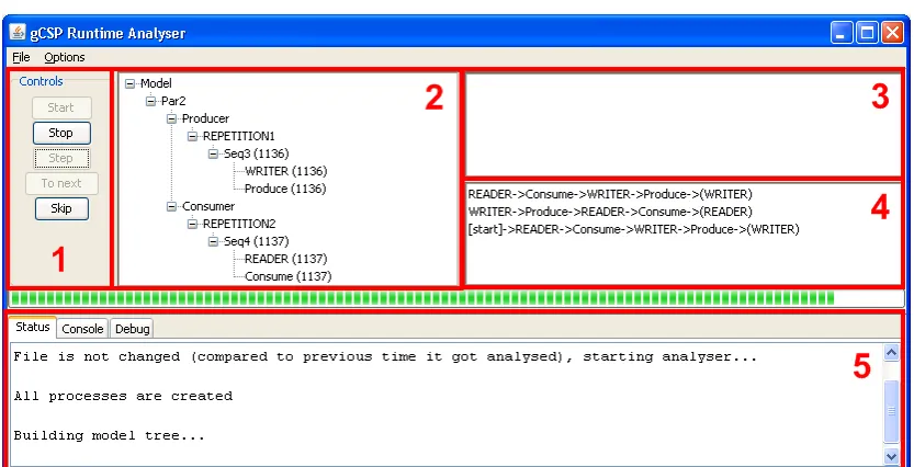
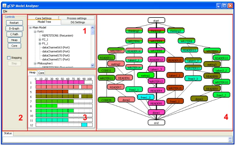
The implementation of both types of communication is described in Section 3.3.1. Last but not least a User Interface (UI) is added to provide interaction between the analyser algorithms and the user. A picture of the UI is shown in Figure 3.2.

(16)

The top left part, numbered 1, contains buttons to control the algorithm after a model is started. Number 2 is the output of the tree recreation algorithm described in Section 3.2.1. Panel 3 initially shows the processes available in the model and during the analysis the processes which are not placed in the model tree yet. The panel is empty in the figure since all processes are placed. The results of the process order algorithm, described in Section 3.2.2, are visible in panel 4. Finally part 5 shows the status of the analyser, other available views are the console line texts and a debugging view, mainly showing the TCP/IP communication. A more complete description of the user manual can be found in Appendix F.

3.2 Algorithms

As briefly mentioned before the runtime analyser makes use of two algorithms. One to reconstruct the model tree and one to determine the order of the execution of the processes. Both algorithms run simultaneously, but the model recreation algorithm finishes when the model tree is completed. The process order algorithm will not stop until the user stops it.

Both algorithms use the state change information of the processes. Before the algorithms can be started the executable needs to initialise its processes. The information send during the initialise stage is required to initialise the analyser as well. The newly created processes are stored in a list waiting to be placed in the model tree. When breakpoint information is received the analyser knows that the initialisation is completed and the executable is ready to run.

3.2.1 Model construction algorithm

Model reconstruction seems a little unnecessary, since the original gCSP model files will be present in most cases. Some reasons to still reconstruct a model are firstly the fact that the gCSP model files are complicated to read, so it is hard to extract information from them. Secondly it might be the case that the model files are not present or they might have been changed in a new version of gCSP. By not using them, the analyser will be not influenced by model file changes. Thirdly the executable which is going to be analysed might be different compared to the model being used. By being independent of the model this problem will not occur. Another advantage is that unused processes automatically become visible when they do not disappear from panel 3.

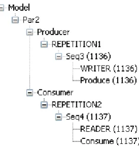
[image:16.595.217.354.573.719.2]

After the executable has created the processes and panel 3 contains these processes, an empty model tree is instantiated. This tree represents the compositional relationships between all pro-cesses. All grouped processes appear on the same branch and all groups themselves also appear on the same branches when belonging together. Processes are grouped to inform the scheduler in the CT library how they should be executed, for example in parallel or sequential order. Figure 3.3 shows such a reconstructed model.

Figure 3.3, A reconstructed model tree

(17)

and the same goes for the processes ‘READER’ and ‘Consume’. Both process groups are grouped with a repetition to make sure they keep repeating until the program is terminated. Finally the two repetition groups are grouped together to make sure they are executed parallelly.

The algorithm monitors the state change information and with a single rule it is able to reconstruct the model tree.

If a process is started or becomes ready for the first time, make it a sibling of the

previously activated process Rule3.1

As Rule 3.1 states a process should be added to the last activated process. The last activated processes is the last process which got finished or blocked, depending on the situation.

Each process that is put in the model tree is removed from the list shown in panel 3 of Figure 3.2. When panel 3 is empty the model reconstruction algorithm is finished.

3.2.2 Process ordering

The second algorithm will try to simplify the model by grouping processes into bigger processes. So less content switching is required, resulting in less used resources when executing the model.

Like the previous algorithm, this algorithm also makes use of the state change information. This time only the state change ‘finished’ is used, since the process order of the chains should represent the order of the processes being finished. This way the chain shows the sequential relation between the processes. In the case that the ‘started’ state would be used the chain order would be messed up, because a process can be started and blocking multiple times before finishing once. Resulting in a chain which would block if it would be implemented.

The algorithm operates in two modi. The first mode is active when the current chain has not reached an endpoint yet. The second mode is for chains which have set their endpoint(s). A chain is ended if a process is added to the chain which already was added. In order to keep things simple, a chain is allowed to include a process only once.

The used notation will be described in the following section. The two modi are described in the next two sections.

Used notation

As described before, the algorithm tries to find static process order chains. When a series of processes is executed during the analysis they become a chain. The notation of the chains in the two sections explaining the algorithm are the same as used in the user interface of the runtime analyser. Figure 3.4 shows an example notation of these chains.

D->C->F->B->(B, D*) B->E->A->C->(E**, D) [start]->A->B->C->D->(B)

Figure 3.4, Example notation of the chains

Each chain has a unique starting process followed by a series of processes and is ended by an endpoint. The endpoint is shown between the parentheses. It consists of either a single process or a group of processes. The endpoint indicates the chain(s) which might become active after the current chain is ended. Asterisks are used to indicate that chain is looped. One asterisk is added when an ending process refers to the beginning of its chain. Two asterisks are added when an ending process is pointing to a processes in the middle of its chain.

When looking at this example, the executable starts at its main starting point ‘[start]’. When the

chain is ended the chain starting withBis activated. At the end of that chain two possibilities are

available. The outcome depends on the internal mechanisms: either the current chain stays active

and continues at processEor the chain starting withDbecomes active. When chainDis ended

(18)

Rules for chains with no endpoint

The rules in this section are responsible for creating and extending new chains. The trace shown in Figure 3.5 is used to explain the rules in this section.

1 2 3

| | |

A->B->C->B->D->E->F->B

Figure 3.5, The used trace

A trace is a sequential order of processes fed to the algorithm. The numbers above the trace indicate the position for the explanation of the rules.

If the state of processpchanges to ‘finished’ addpto the end of the active chain. Rule3.2

Rule 3.2 is the most basic rule to create new chains. When position 1 is reached, it results in a new

chain with processesA,BandCadded, as shown in Figure 3.6.

A->B->C

Figure 3.6, A new chain

At position 2 processBis finished for a second time. Since it is not allowed to add a process twice

to a chain, Rules 3.3 and 3.4 are required.

If processpgot added but it was already present in the chain, it will become an

endpoint of the chain. Rule3.3 If a chain gets ended by processp, the chain starting withpis looked up.

If the chain is not available a new chain starting withpwill be created. The found or newly created chain will become the new active chain.

Rule3.4

Rule 3.3 defines when a chain should be ended. When a chain that starts with process Bis not

found, Rule 3.4 states that a new chain should be added. The result is shown in Figure 3.7.

B

A->B->C->(B)

Figure 3.7, A Second chain is added

When position 3 is reached processBagain applies to Rule 3.4. This time a chain starting with

processBis found: the current active chain. No new chain needs to be added and the current chain

is ended as shown in Figure 3.8.

B->D->E->F->(B*) A->B->C->(B)

Figure 3.8, The complete trace converted to chains

These three rules are sufficient to add processes to new chains. New chains always have an unique starting process and do not have processes added twice to them.

A->B->C->(A*) A->D->E->(A) A->F->G->(A)

Figure 3.9, No unique starting processes

Figure 3.9 shows chains without unique starting processes. The first chain ends with A*. No

problem occurs here since the current chain is reactivated when it ends. The other two chains result in a problem, since it is unclear which chain is activated next. Only chain which is certainly not activated is the current chain.

Figure 3.10 shows the problem arising without Rule 3.3 being active. The end process refers back

to the processBin the middle of the chain. Problem is the fact that two processesBare present in

(19)

A->B->C->B->D->E->(B**)

Figure 3.10, No unique processes in chain Rules for chains with endpoint(s)

When the active chain is ended already, the rules should check if the chain is correctly created. Therefore the position in the currently active chain should be remembered. To explain the rules in this section the trace is extended, as shown in Figure 3.11.

1 2 3 4 5

| | | | |

A->B->C->B->D->E->F->B->D->G->H

Figure 3.11, The extended trace

First of all it should be checked if the active chain was at its end. Position 3 ends the chain starting

with B shown in Figure 3.8. Rule 3.5 performs this check and makes the current chain active

again.

If the finished process p is at the end of the chain, find the chain starting with

processpand make it the active chain. Rule3.5

When the chain is not ended, the current position in the chain should match the finished process resulting in Rule 3.6.

If the current position in the chain does not match the finished processpthe chain

must be split. Rule3.6

At position 4, processDgot ended. Previously processBwas ended, so processDis expected next.

No problems arise since the expected and the finished processes match. At position 5 processG

finished, which is not the expected process afterD. According to the rule, the active chain should

be split.

Splitting chains is a complicated task, since the resulting chains still need to match the previous

part of the trace. For the current trace the active chain should be split after processD, since that

process was still expected. Rule 3.7 defines the steps to be taken in such a situation.

The active chain should be split at processewhen processpis unexpected and a chain starting with processeis not yet present.

To split a chain:

End current chain before processe and put the processes afterein a new chain starting with processe

Create a new chain starting with processpand make it the active chain.

Rule3.7

It results in a new chain starting withEcontaining the remainder of the active chain. A new chain

is created starting with processGand is made active. The resulting chains are shown in Figure

3.12.

G

E->F->(B) B->D->(E,G) A->B->C->(B)

Figure 3.12, Chains after splitting chainB

When following the trace from the start till position 5, the chains in the figure are matching the

given trace again. The active chain is the chain starting with processGand is not yet finished so

the rules of the previous section apply to it.

(20)

1 2 3 4 5 6 7

| | | | | | |

A->B->C->B->D->E->F->B->D->G->H->B->D->G->H->I

Figure 3.13, The final trace

Till position 6 no problems occurred, Figure 3.14 shows the result till this position.

G->H->B->D->(G*) E->F->(B) B->D->(E,G) A->B->C->(B)

Figure 3.14, The chains till position 6

At position 6 processHis finished and expected, so position 7 is reached. A problem occurs at

position 7: ProcessIis finished but processBis expected, so the chain should be split. Problem

is, a chain starting with processB is present already. Having two chains starting with the same

process is not allowed. However, it is clear that the processes after processHmatch the chain

starting withBexactly. Rule 3.8 provides a solution for these situations.

The active chain should be split at processewhen processpis unexpected, but a chain starting with processeis present already.

Compare the remain processes afterewith the chain starting with processe

If both parts are equal, remove the remaining processes in the active chain starting at processe.

And create a new chain starting withpand make it the active chain.

If the comparison did not succeed, the static process order cannot be determined and the algorithm should stop.

Rule3.8

Figure 3.15 shows the result after applying the rule.

I

G->H->(B,I) E->F->(B) B->D->(E,G) A->B->C->(B)

Figure 3.15, The chains after position 7

ProcessIis active and can be created using the rules of the previous section again.

If the comparison of the rule failed, it indicates that two unequal chains starting with the same process should be created. This situation is not supported by the algorithm, because it results in a badly construct model. The internal mechanisms of the CT library could not determine which of the two chains should be used in a certain situation.

A simple example which has a chance to fail the comparison would be a ‘one2any channel’: one process writes on the channel and multiple processes are candidates to read the value. If the reading order of these candidate processes is not deterministic, Rule 3.8 fails.

3.3 Design and implementation

3.3.1 Communication

In order to be able to follow the execution patterns of a program, the algorithm has to be fed with usable information. In order to get hold of this information some sort of communication is required. Two communication types are used when analysing the executable: command line output and TCP/IP communication. This is shown in Figure 3.1.

Command line communication

(21)

by the analyser. The output texts are send as two character streams, one for the regular output texts (stdout) and one as error output texts (stderr). Both streams are being watched by a thread in the analyser and the texts are displayed in the console tab of the user interface. The analysis algorithms do not make use of this information.

The command line communication allows for bidirectional communication. An input character stream (stdin) is available as well, but the analyser does not make use of it.

TCP/IP communication

The second communication type is much more sophisticated, since it makes use of an available protocol. The protocol is part of the animation functionality of gCSP and allows for influencing and monitoring the running processes.

After the executable is loaded it opens a TCP/IP port and listens to incoming connection requests. When a request is received and the connection is made, the executable starts initialising its pro-cesses. After the initialisation is done, the executable waits on commands to start or step the processes. During the creation and state changes of the processes information is send over the communication channel to the analyser. An intermediate object receives and filters this informa-tion and sends it to the algorithms. More informainforma-tion about the usage of these commands can be found in Section 3.3.2.

3.3.2 Controlling the execution flow

In order to influence the flow of the execution of the processes the animation functionality is used. Commands are send to the executable instructing to start, step or stop the execution.

The executable (or more precisely the CT library) sends status information to notify the listening application about state changes, the creation of new processes, breakpoints being placed, error information and logging information. This information is used to find out about the situation of the executable and the model it contains. So the analyser is able to reconstruct this model without having knowledge of the original gCSP file. How this information is used is described in Section 3.2.

3.4 Results

This section describes the results of the analyser, first a functional test will be performed. Next usability tests are performed to see whether the results of the analyser can be used when more realistic models are used.

3.4.1 Functional test

As a functional test a simple producer consumer model is created, as shown in Figure 3.16. Besides just sending data over a channel it also calculates the time passed since the executable was started. So it is possible to compare the model with an optimised version later on.

(22)

The model is loaded in the analyser, which automatically generates code, compiles and creates an executable. Figure 3.17 shows the result of the analyser.

READER->Consume->WRITER->Produce->(WRITER) WRITER->Produce->READER->Consume->(READER)

[start]->READER->Consume->WRITER->Produce->(WRITER)

Figure 3.17, Three process chains for the ProducerConsumer model

Two chains are created which seems to be the same, except that they have a sort of ‘phase change’. A starting chain is shown as well, but it is exactly the same as the READER chain, so it can be neglected. Next the channel is changed to a buffered channel with a size of 1, see Figure 3.18. Only one chain is left which has a circular reference to itself, hence the asterisk at the end. The starting chain is the same again and can be neglected.

WRITER->Produce->READER->Consume->(WRITER*)

[start]->WRITER->Produce->READER->Consume->(WRITER)

Figure 3.18, Result for ProducerConsumer test with a buffered channel

When comparing both results their execution order looks the same on a first glance:

WRITER->Produce->READER->Consume

But the ending processes are different. In the first result it points to READER which results in:

WRITER->Produce->READER->Consume->READER->Consume->WRITER->...

And at the second result it points to WRITER resulting in:

WRITER->Produce->READER->Consume->WRITER->Produce->...

So depending on the channel type, different behaviour is found by the analyser.

Another difference is the amount of chains, the first result has two chains because references are only allowed to the start of the chain. So a new chain has to be added in order to reference to the start. The second result references to the start of itself which is allowed. The second result cannot directly be used to create an optimised model, since the channel needs two processes to be ready before sending data. It will not work with only one chain and thus one process.

Figure 3.19 shows the simplified version of the original model. It has only two processes which contains combined code from the original model in order to represent the two chains found. Also the repetitions are replaced by an infinite while-loop in the code. Resulting in a model which is as optimal as possible.

Figure 3.19, The simplified ProducerConsumer model

When the runtime analyser tries to analyse it will not give results. Because non of the processes will finish. Due to the added infinite while-loops, no finish state information is send. This is not a problem since it is more interesting to compare the speeds of both models.

(23)

The original gCSP model needs quite some remodelling in order to comply to this test setup, as can be seen in Figure 3.20. The simplified model consists of two code blocks, so it is easy to implement the test setup.

dataChannel1

Produce

p:Double !

WRITER

[image:23.595.126.484.126.351.2]

* REPETITION1 [isRunning]

isRunning

isRunning:Boolean PROD_INIT

dataChannel1

Consume

?

READER

*

REPETITION2 [now - start_time < 6000 | producerCanBeStopped]

c:Double isRunning

FINISH

now:Integer start_time:Integer

isRunning:Boolean INIT

f:FILE* current:Integer

producerCanBeStopped:Boolean

Figure 3.20, The ProducerConsumer model with measurement added

The figure shows that a lot of extra processes unfortunately are required in order to perform the measurements. This is the result of the lack of a init and finish code block possibility for pro-cesses. So the results will not be very accurate since extra context switched are introduced by the measurement system.

The found results are shown in Figure 3.21. The y-axis shows the amount of data produced and consumed for the corresponding interval. The more data is processed the better, since it indicates that the model is running faster.

0 10000 20000 30000 40000

0 10 20 30 40 50 interval

data/interval

Original model

Optimised model

Figure 3.21, Measurement results

It is clear that the optimised model indeed has better results compared to the original model. The average factor between both models is 1.298, so the optimised model is about 30% faster. The minimum and maximum factors are 1.293 respectively 1.304. So doing multiple runs seems to result in a steady measurement result.

(24)

Caution should be taken when the analysed model is using recursions or alternative channels. This may lead to processes which are not used during the analysis. This becomes visible when panel 3 of Figure 3.2 still contains unused process, even though the analysis is finished. In such unexpected situations the user should recheck the original model for design errors. Otherwise one should remember to add the unused processes as well, when optimising the model using the results of the analyser.

3.4.2 Usability tests

The previous section showed that the analyser is working and that the optimisation indeed is better, compared to the original. This section describes the analysis results of several more realistic models to evaluate the usability of the tool.

Production cell

Figure 3.22 shows the used model of the production cell (van den Berg, 2006). This is the analysis model, which differs greatly from the model to actually control the production cell. The analysis model contains the blocks available on the production cell, but not the actual controlling parts.

Figure 3.22, production cell

The processes define parts of the production cell which all are connected by transport mechanisms, like a belt or a gripper. In the model the processes are connected by channels to simulate these connections. Most of the blocks only read from their input channel and write to their output channel. The BlockInserter inserts a block into the InsertBuffer which will insert the block in the circular channels when the channel to FeederBelt is empty. After that the block will circle forever in the model. The used BlockInserter only inserts one block, but it would be possible to stress test a model by inserting multiple blocks. At a number of seven inserted blocks the model should deadlock, since all blocks will be waiting for each other.

The results of one circling block can be viewed at Figure 3.23. The chains were too long to fit on a single line so they are separated by empty lines.

WRITER4->READER5->READER6->WRITER5->WRITER3->READER4->READER7->WRITER6->WRITER2->READER3 ->READER8->WRITER7->READER1->WRITER8->(WRITER4*)

WRITER5->READER6->WRITER4->READER5->WRITER3->READER4->READER7->WRITER6->WRITER2->READER3 ->READER8->WRITER7->READER1->WRITER8->(WRITER4)

WRITER6->READER7->WRITER5->READER6->WRITER4->READER5->READER4->WRITER3->WRITER2->READER3 ->READER8->WRITER7->READER1->WRITER8->(WRITER5)

[start]->WRITER3->READER4->WRITER2->READER3->WRITER7->READER8->WRITER6->READER7->WRITER5 ->READER6->READER5->WRITER4->READER1->WRITER8->(WRITER6)

Figure 3.23, Result of the analyser for the production cell model

(25)

‘[start]’ and ending with chain ‘WRITER5’. After the starting phase is finished the model will

circle in top chain ‘WRITER4’.

The actual result of the analyser consists of one chain, resulting in one process when implementing it. It might be clear that this will not work, since a channel should be connected between two processes. A solution, for a single core target, would be replacing the channels for variables. Now the sequential scheduled code blocks can write and read a variable without getting blocked.

Another problem is checking for the correctness of the result. The Reader and Writers are not nicely following up. So it becomes nearly impossible to check whether the correct order is found. Since the analyser is using the runtime information the order should be correct as is was with the ProducerConsumer model. All more realistic models are complex, as shown with this example. The results of the analysis are hard to be checked and without knowledge of the inner workings of the CT library it becomes virtually impossible.

This model showed that an alternative channel might result in unused processes. Panel 3 (Figure

3.2) keeps displaying ‘WRITER9’, ‘WRITER10’, ‘WRITER11’, ‘WRITER12’, ‘WRITER13’ and

‘READER2’. The model was build to check for deadlocks when seven block are inserted into the production cell. The analysis shows that only one block is inserted and keeps circling around. So it can be concluded that the analyser also can be used, to quickly check if a model is behaving as one should expect when using these channel types.

Dining Philosophers

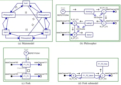
A well-known concurrency problem is the dining philosophers dilemma. Concurrency is a situa-tion with multiple processes running interleaved on a single core. Without proper implementasitua-tion deadlocks might occur when two or more processes are waiting on each other. Figure 3.24 shows a gCSP model of this dilemma.

(a) Mainmodel (b) Philosopher

[image:25.595.102.516.431.724.2]

(c) Fork (d) Fork submodel

Figure 3.24, Dining philosophers

(26)

philosopher. The only problem is the fact that the amount of forks is equal to the amount of philosophers. A hungry philosopher first grabs his left fork and next his right one, when both forks are obtained he starts to eat. When stuffed he drops both forks making them available for his neighbours, and start thinking again until he gets hungry.

A problem happens when a fork is taken by a neighbour philosopher, since the philosophers have their matters they patiently wait until the fork is released. The real dilemma occurs when all philosophers obtained one fork and are waiting for the other fork. They all will starve to death since a deadlock situation occurred.

The model consists of three philosophers with their three forks. Sub models of the philosophers and the forks are shown as well. The names of the model parts are abbreviated to keep the chains as short as possible. Examples of the abbreviations are: ‘P1’ for philospher1 and ‘F1’ for fork1. The model is implemented correctly with respect to deadlocks, so it is possible to run using the runtime analyser. Its results can be found at Figure 3.25 and again the results are complex.

thinking2->W_F1_P2->F1_P2_free->R_F1_P2->F1_P2_taken->W_P2_F1->W_P2_F2->eating2 ->R_F2_P2->F2_P2_taken->W_F2_P2->F2_P2_free->R_P2_F2->R_P2_F1->done2->(thinking2*)

[start]->thinking1->thinking2->thinking3->W_P2_F1->R_F1_P2->F1_P2_taken ->W_P2_F2->eating2->R_F2_P2->F2_P2_taken->W_F2_P2->F2_P2_free->R_P2_F2 ->R_P2_F1->done2->(thinking2)

Figure 3.25, Result of the analyser for the dining philosophers model

The circular chain ‘thinking2’ is the only chain available, except for the starting chain. So the

optimised model cannot be implemented directly using the results, like the production cell model.

When comparing the top chain with the graphical model, it becomes clear that not all processes get activated and finished during runtime execution. This behaviour is the result of the implementation of the parallel construct of the CT library. The processes are not really parallelly running, but get scheduled using the scheduler of the CT library. This scheduler prefers to restart the last finished process if possible, resulting in only one philosopher being able to eat and the other two suffering of starvation.

So the runtime analyser can be used to detect badly constructed models, especially since these processes also are visible in panel 3 of Figure 3.2.

A solution to the dining philosophers dilemma is to assign a butler. A hungry philosopher asks this butler for his forks. The butler grants permission when both forks are available, before granting permission the butler reserves the forks. Now the philosophers will not starve to death, assuming none of the philosophers is greedy and will not release his forks, since they always get both forks when permission is granted.

The corresponding model and the analyser results are shown in Figures 3.26 and 3.27. The philoso-pher and the fork sub models are slightly changed, since they have interaction with the butler as well, but not extensively and therefore are not shown.

The results show that the model is better constructed and all philosophers are thinking and eating as they should.

Plotter model

The previously analysed models are not real controllers, but demonstrate the different results of the analyser. The plotter model, shown in Figure 3.28, is an actual controller model able to control a plotter.

(27)

Figure 3.26, Dining philosophers with butler

R_F2_R->F2_released->W_P3_B->R_B_P3->W_B_P1->R_P1_B->W_P1_CF1->R_F1_C->F1_claimed ->W_P1_CF3->P1_eating->R_F3_C->F3_claimed->W_P1_RF1->R_F1_R->F1_released->W_P1_RF3 ->P1_thinking->R_F3_R->F3_released->W_P1_B->R_B_P1->W_B_P2->R_P2_B->W_P2_CF2->R_F2_C ->F2_claimed->W_P2_CF1->P2_eating->(R_F1_C)

R_F1_C->F1_claimed->W_P2_RF2->R_F2_R->F2_released->W_P2_RF1->P2_thinking ->R_F1_R->F1_released->W_P2_B->R_B_P2->W_B_P3->R_P3_B->W_P3_CF3->R_F3_C

->F3_claimed->W_P3_CF2->P3_eating->R_F2_C->F2_claimed->W_P3_RF3->R_F3_R->F3_released ->W_P3_RF2->P3_thinking->(R_F2_R)

[start]->W_B_P1->R_P1_B->W_P1_CF1->R_F1_C->F1_claimed->W_P1_CF3->P1_eating->R_F3_C ->F3_claimed->W_P1_RF1->R_F1_R->F1_released->W_P1_RF3->P1_thinking->R_F3_R

->F3_released->W_P1_B->R_B_P1->W_B_P2->R_P2_B->W_P2_CF2->R_F2_C->F2_claimed ->W_P2_CF1->P2_eating->(R_F1_C)

Figure 3.27, Result of the analyser for the of dining philosophers with butler model

The motion sequencer uses a provided file to create a motion path for the pen. The motor con-trollers block contains a 20-sim model to control the X, Y and Z motor of the plotter. The safety block contains safety checks and is able to disable the X, Y or Z motor signal to make sure no un-safe situations occur. The last block, Scaling, scales the X, Y, Z and VCC signals within expected value ranges so the plotter received to correct signals.

After the runtime analyser finished the analysis, the results visible in Figure 3.29 are obtained.

Even such a big model has a defined running order, changing the input file does not change this result. When the complete input file is processed the executable exits and the analyser finishes the analysis. The duration depends on the amount and type of the drawing commands in the input file.

It is virtually impossible to validate the results. From ‘[start]’ to ‘WRITERZ’ the order seems

reasonable. After that part the optimised channel effects start to play a role and ‘HPGLParser’

is finished for the second time, even before the rest of the model has been finished.

These so called optimised channel effects are the result of a channel optimisation in the CT library (described in (Hilderink, 2005) section 5.5.1). This optimisation only allows context switches when really needed. So for example after reading a result from the channel, the reading process stays active and could try to read a second time. This second time the channel will be empty and the reader blocks and the writing process will be activated again. However, before the reader tries to read the channel, other non-blocking processes could have been finished and put in the chains. This results in hard to explain analysis results.

(28)

Figure 3.28, Plotter model

READER17->WRITER4->READER16->WRITER3->READER13->WRITER2->READER8->WRITER1->READER12 ->READER11->READER10->READER9->WriteToTimer->Safety_X->READER14->READER15->Safety_Y ->Safety_Z->READER1->READER2->READER3->WRITERX->PWMY_Safe_WRITER->READER19

->PWMZ_Safe_WRITER->READER20->PWMX_Safe_WRITER->READER18->READER4->WRITERY ->DoubletoShortConversion->WRITER11->WRITER12->WRITER13->READER5

->LongtoDoubleConversion->Controller->WRITERZ->(READER21)

READER21->DoubletoBooleanConversion->WRITER14 ->VCCZ_Safe_WRITER->(READER17, HPGLParser)

WRITER1->READER8->WRITER2->READER13->WRITER3->READER16->WRITER4->READER17

->WriteToTimer->READER12->READER11->READER10->READER9->READER1->READER2->Safety_X ->READER14->READER15->Safety_Y->Safety_Z->READER3->WRITERX->READER4

->WRITERY->PWMY_Safe_WRITER->READER19->PWMZ_Safe_WRITER->READER20->PWMX_Safe_WRITER ->READER18->READER5->LongtoDoubleConversion->Controller->WRITERZ

->DoubletoShortConversion->WRITER11->WRITER12->WRITER13->(HPGLParser)

HPGLParser->(WRITER1, READER21)

[start]->HPGLParser->WriteToTimer->READER1->READER2->READER3->WRITERX->READER4 ->WRITERY->READER5->LongtoDoubleConversion->Controller->WRITERZ->(HPGLParser)

Figure 3.29, Result of the analyser for the plotter controller

3.30. The last ‘HPGLParser’ references back to the first one and the loop is complete. This

complex order also is a result of the channel optimisations.

[start]->HPGLParser->WRITER1->HPGLParser->Reader21->READER17->READER21->(HPGLParser*)

Figure 3.30, Execution order of the chains

3.5 Conclusions

First of all the runtime analyser seems to work as expected. It is able to analyse most (pre-compiled) models, only rare situations are known for which the analyser will stop prematurely.

The sets of rules are defined by using relevant tests containing most common situations. The defined rules are sufficient for deterministic models and for simple non-deterministic models as well. However, the rules are not proved to be complete. When new (non-deterministic) situations are analysed it might be possible that new rules are required.

Currently, the results of the analysis are based on a single thread scheduler. When multiple-cores are used and the scheduler is able to schedule for multiple threads the analysis results are undefined. Processes will be running really parallel and received state changes are originating from unknown threads. To solve this problem the received state changes should be accompanied by thread information. The analysis algorithms can construct the chains for each thread separately using this extra information.

(29)

runtime analyser tool. The tools would not be able to notice the difference and it becomes possible to do analysis for models which runs on their target system.

Even though the results are likely to become very complex, usable information can be obtained as shown by the usability tests. A simple result to obtain is whether all processes are used at runtime. Processes which are unused will not become part of the model tree. Of course these processes might become active depending on external inputs, but this information can be used to take a closer look at least.

A more complex usage of the results is to actually implement them. Using the chains it becomes possible to create big processes having the processes of each chain in them. By replacing channels, which stay in the same process, with variables the processes will not block and also become even simpler. These steps result in an optimised model which requires less system resources and runs faster.

(30)

4 Choice of the model input mechanism

In order to read the gCSP2 models a suitable input mechanism should be provided. The current gCSP files are stored using the Extensible Markup Language (XML) (World Wide Web Consor-tium, 2008) as stated before in Section 2.3. This is a well-known and a well-defined format and is a good basis to store the gCSP2 models in. A lot of tools are available to read and parse these files, Section 4.1 describes four possibilities to read XML files using these tools.

It is also possible to create dedicated gCSP files and accompanying readers using a scanner-parser combination. A scanner, or tokeniser, is a program which recognises lexical patterns in a stream of characters. A parser converts the tokens, generated by a scanner, into a data structure. Scanners and parsers are quite complex and therefore generators are available. The two best known scanner-parser generators are described in Section 4.2.

The final section presents the conclusion and selected input method used in the rest of the project.

4.1 XML readers

A XML reader is a piece of software which is designed to read XML files. Mostly they are part of a XML library which is also able to write XML files and to present the XML files in a data structure with all kind of usage support methods. A general disadvantage for XML readers is that they are bloated, they provide lots of functionality of which only a part will actually be used.

This section describes three software libraries which are able to read XML files. The first type consists of the generic XML libraries. These generic XML libraries can be found on the Internet in a lot of varieties. Next XMLSpy is described. This is a complete software environment to create XML files and files related to them. Finally the Eclipse Modeling Framework is described, this is a plug-in for the Eclipse environment.

4.1.1 Generic XML library

Many generic XML libraries can be found on the Internet and many flavours are available each with their own advantages and disadvantages. One of the most well-known libraries is MSXML, which is provided within the Windows operating system. The latest version is MSXML 6.0 (Mi-crosoft Corporation, 2008). Other well-known XML libraries is Libxml2 (Veillard, 2008) and TinyXML (Thomason, 2008), which are available on many platforms and quite popular in the open source scene.

Depending on which flavour is picked, extensive documentation might be available, which could result in an easy to use library. As the term ‘generic’ already implied it is not possible to use a meta-model to fit the model data in. Any XML tag is allowed, which obviously is a disadvantage.

4.1.2 gCSP

The current version of gCSP also stores its model using XML files, so it could be used to read the XML files as well. The main reason for writing a new meta-model is because of the complexity and messy implementation of the gCSP files. The gCSP code is not very clean, since a lot of patches are added over the years. It is based on the Java XML serialiser and thus has the same advantages and disadvantages as the generic XML libraries.

4.1.3 XMLSpy

(31)

a XSD (XML Schema Definition), which describes the syntax of the XML file. This XSD file can be used to generate Java, C++ or C# code.

The generated code is mainly a data storage structure, with a provided interface to a generic XML library to load and store its contents. Some of the supported libraries are MSXML, Java API for XML Processing (JAXP), and Microsoft System.XML. The used library is mainly dependent on the used programming language. So the only real advantage of using XMLSpy over a generic XML library seems to be the graphical way of defining the syntax or so called meta-model of a XML file. The generated code makes use of the generic XML libraries. So the advantages and disadvantages of generic XML libraries are also valid for a XMLSpy solution.

4.1.4 Eclipse Modeling Framework

The Eclipse Modeling Framework (EMF) (The Eclipse Foundation, 2008) is a plug-in, of the Eclipse environment, which is an open source development environment. EMF provides support for modelling models, so it can be used to create meta-models. After a meta-model is created, the EMF is able to generate code. This code defines the meta-model and provides methods to store, read and modify the model. An available (de)serialiser provided with EMF, supports XML file formats. A major advantage is the fact that it is possible to modify the code without losing the modifications when the meta-model code is regenerated.

A small disadvantage of Eclipse and EMF is the complexity of the environment and all of its features. Before one is able to fully use it quite some experience is required, fortunately lots of documentation and tutorials are available.

4.2 Scanner-Parser generators

As stated before, it is also possible to read the XML files using a scanner-parser combination. Both are pieces of software, which can be combined into a single application. The combination of both is able to read data and convert it into another set of data. In this case from a gCSP file to a data structure in the memory. Actually the XML readers described above also contain some sort of scanner-parser combination to read the files, and to write the contents into the memory. However, using a custom created combination has some advantages. Building these would be a lot of work, thus automated generators are available.

These generators are fed with a language definition and generate the required code to read a stream of characters of this specified language. First the stream of characters is converted into a stream of tokens by the scanner. These tokens consist of characters which together are a building block of the language. This stage is called the scanning, or lexing, stage and is followed by one or more parsing stages. During this stage the tokens are combined into new tokens and finally the obtained information is stored. Without the scanning stage the process would be too complicated, hence the two stages.

As a result the obtained software is only able to read the models and put it into a dedicated struc-ture. It results in less bloated software in comparison to the generic XML libraries. Since these libraries are able to perform all kinds of operations on the XML specific data structures. Another major advantage is the possibility to have multiple parsing stages, so it will be possible to im-plement the required algorithms in the parser stages. This will seamlessly link with reading the documents.

A disadvantage of using a scanner-parser combination is the fact that it only is able to load a model. After modifying a model or generating a new one it has to be stored again, which would require another piece of software specially made for this task.

(32)

an error or warning. All these kind of differences influences the complexity and speed of the scanners and parsers.

4.2.1 Flex and Bison

The most well-known parser generator combination probably is the Flex (The Flex Project, 2008) and Bison (Free Software Foundation, 2008) combination. Both are open source programs and around for many years.

Bison is a parser generator that converts an annotated context-free grammar into an LALR(1)

or GLR parser for that grammar. LALR is short for LookAhead Left-to-rightRightmost and

is and a specialized form of the LR parser. This is a type of parser that reads input from Left

to right and produces aRightmost derivation. The rightmost derivation, contrasted by leftmost

derivation, is a way how the tokens and sub-tokens are linked to each other. Look ahead parsers take more of the parser context into account and are therefore more specific compared to non-look ahead parsers. The number in the parentheses tells how many unconsumed tokens, the look ahead property, are allowed. The higher this number the more complex the parser will become, since more combinations will apply.

GLR is short for Generalized Left-to-right Rightmost and thus also a LR parser. Generalised

means that it allows for ambiguous grammars in contrast with the LALR parsers. Ambiguous grammars have constructs which can be interpreted in multiple ways. An example is the following

(partial) line of C: x ∗ y;. This can be read as ‘x multiplied by y’ or as ‘a declaration of y which is

a pointer of the type x’. Depending on x being a variable or a type declaration, the first respectively the second should be chosen by the parser. It might be clear that ambiguous languages are very complex to parse.

Because of their familiarity a lot of documentation and examples can be used. So it is very easy to start using them. A disadvantage is the lack of a (graphical) interface since they are command line tools. The output of this combination is specialized on C/C++ and converting this to Java incorporates a loss of code quality of course.

4.2.2 ANTLR

ANTLR (Parr, 2008), which is short for ANother Tool for Language Recognition, is able to

generate a scanner-parser combination. Having scanners and parsers generated from the same input has a nice advantage that strings being used in the parser parts automatically are created as tokens in the generated scanner. ANTLR makes use of a so-called StringTemplate, created by the same author, which enables the possibility to generate code for a variety of target languages. It is even possible to add custom or unavailable languages.

The generated parser is a LL(*) type parser. Where LL is short forLeft-to-rightLeftmost, which is

the opposite of the generated bison parser. The * indicates that it can use a variable amount tokens to look ahead depending on the current language rule being processed. Because of this look ahead type it is not possible to use lookup tables and additional code is generated to replace them. In order to allow even more complex language definitions ANTLR also supports backtracking. This is useful when sub-rules are used and the parser has to fit the available tokens to the processed rule and to the used sub-rules. It can try several combinations without needing huge look ahead combinatorics, since it will just take a step back and try another possibility when the current one does not fit.

(33)

not table entries. Is it also possible to create the ANTLR rules using a graphical editor called ANTLRWorks. It shows the rules as flow diagrams. It also is able to interpret input and use a simple debugger to show the steps taken to produce the parsed output.

4.3 Conclusion

Table 4.1 shows an overview of the advantages and disadvantages of the readers, most columns are clear but some vague columns might need a short description: The ‘Java’ column indicates that the reader (and meta-model if applicable) can be created in Java, the ‘meta-model’ column that the reader has a meta-model to check the files with and ‘complexity’ indicates how complex or difficult the creation of the reader is.

Ja

v

a

Code

cleanness

Meta-model

Editor

/

En

vironment

Free

/

Open

source

Comple

xity

Generic XML library + - - 1 ₊ ₊

gCSP + - +/- 1 +

-XMLSpy + - + +/- - +

Eclipse EMF + - + + +

+/-Flex & Bison - + + - +

-ANTLR + + + +/- +

-1 _{Since no meta-model is available, an editor is not required}

Table 4.1, Requirements for the readers

The desired language to read the gCSP2 models is Java, because the code should be reusable by the future version of the gCSP editor. Since the new editor is going to read the models, a simple reader is required as well so it will be easy to update the reader when the model gets extended. These two restrictions drop the scanner-parser generators, especially since the complexity requirement is weighted heavily.

Eclipse also is rated as mediocre complex, but it is expected that it is much easier to learn to use eclipse than a scanner-parser generator. So the +/- rating would lean more to the ‘+ side’.

It also is nice to have an editor or environment to create the gCSP meta-model, especially if the meta-model editor could be part of the code development environment. So the generic XML libraries will be dropped from the optimal choice, XMLSpy has a +/- rating because the environ-ment only generates code which needs to be used in another environenviron-ment. This leaves Eclipse EMF being favourable compared to XMLSpy.

XMLSpy is a very nice and easy to use editor, it is very user friendly and attractive. Maybe the user-friendliness is a little over the top. Another drawback is the fact that it is commercial software, a free 30-day trial can be obtained, but afterwards the user is expected to pay. These arguments combined with the badly rated environment leaves the choice to Eclipse EMF.