Computer Model for Evaluating Multi Target Tracking Algorithms

(1)

ISSN Online: 2327-4026 ISSN Print: 2327-4018

DOI: 10.4236/ojmsi.2019.71001 Nov. 8, 2018 1 Open Journal of Modelling and Simulation

Computer Model for Evaluating Multi-Target

Tracking Algorithms

Garret Vo, Chiwoo Park

Department of Industrial and Manufacturing Engineering, Florida State University, Tallahassee, FL, USA

Abstract

Public benchmark datasets have been widely used to evaluate multi-target tracking algorithms. Ideally, the benchmark datasets should include the video scenes of all scenarios that need to be tested. However, a limited amount of the currently available benchmark datasets does not comprehensively cover all necessary test scenarios. This limits the evaluation of multitarget tracking algorithms with various test scenarios. This paper introduced a computer si-mulation model that generates benchmark datasets for evaluating mul-ti-target tracking algorithms with the complexity of multitarget tracking sce-narios directly controlled by simulation inputs such as target birth and death rates, target movement, the rates of target merges and splits, target appear-ances, and image noise types and levels. The simulation model generated a simulated video and also provides the ground-truth target tracking for the simulated video, so the evaluation of multitarget tracking algorithms can be easily performed without any manual video annotation process. We demon-strated the use of the proposed simulation model for evaluating track-ing-by-detection algorithms and filtering-based tracking algorithms.

Keywords

Performance Evaluation, Multi-Target Tracking, Computer Model, Simulation

1. Introduction

A multi-target tracking problem is to estimate the trajectory of multiple targets as they move and interact with each other in a sequence of images, estimating targets’ locations and velocities [1] [2]. A multi-target tracking problem was driven primarily by aerospace and defense applications, such as radar, sonar, guidance, and navigation [1] [3] [4]. With the advancement in high performance How to cite this paper: Vo, G. and Park,

C. (2019) Computer Model for Evaluating Multi-Target Tracking Algorithms. Open Journal of Modelling and Simulation, 7, 1-18.

https://doi.org/10.4236/ojmsi.2019.71001

Received: October 8, 2018 Accepted: November 5, 2018 Published: November 8, 2018 Copyright © 2019 by authors and Scientific Research Publishing Inc. This work is licensed under the Creative Commons Attribution International License (CC BY 4.0).

(2)

DOI: 10.4236/ojmsi.2019.71001 2 Open Journal of Modelling and Simulation computing and the availability of inexpensive sensors and cameras, multi-target tracking problem has become popular, and it has grown into an established dis-cipline [5] [6] [7]. Currently multi-target tracking algorithms find many applica-tions in computer vision [2], oceanography [8] [9], robotics [10] [11], and re-mote sensing [12].

Many multi-target tracking approaches have been extensively studied. A pop-ular approach is a tracking-by-detection method that uses an existing target de-tection algorithm to detect targets in images and solves an optimization problem for associating and tracing the detected targets over a time horizon [13]-[22]. Another popular approach is a filtering-based approach, which explicitly models the behavior of targets with a linear or non-linear state space model and esti-mates the system states (typically target locations) using Kalman filtering [23] [24] [25], particle filtering [26] [27] [28] or other MCMC samplers [29] [30] [31] [32].

The performances of the existing approaches vary depending on the com-plexities and types of the video scenes which they applied to, and there is no single method that universally works best for all test videos. It is often very difficult to choose a good tracking algorithm among many algorithms that can handle the video complexities existing in an application of interest. The best way of evaluating and choosing a multitarget tracking algorithm is to use test video datasets collected directly from the application of interest. Howev-er, the evaluation with the test video is often very time-consuming because mostly no ground-truth is available for the test video datasets, for which users may need to spend significant time on manually tracking and annotating targets in the test video. The manual annotation is subject to many human operators’ errors. Using public benchmark datasets coming with ground-truth, such as PETS [21] [33] [34], ETH dataset [35] [36], and Technical University of Darmstadt (TUD) dataset [37] [38] [39], might be an alternative, but the benchmark datasets sometimes do not give any good guidance on the evaluation, because the types of targets and the complexities of the tracking events in the public benchmark datasets are not comparable to those existing in the applica-tion of interest. In addiapplica-tion, the ground-truth of the public benchmark datasets was manually annotated by human operators using video annotation tools, and the quality and information in the ground-truth vary significantly [40].

(3)

DOI: 10.4236/ojmsi.2019.71001 3 Open Journal of Modelling and Simulation The remaining of this paper is organized as follows. In Section 2, we review the public benchmark datasets popularly used for multitarget tracking, and the performance metrics that have been used for evaluating multitarget tracking al-gorithms. In Section 3, we describe our simulation model. In Sections 4 and 5, we present an example of applying the simulator for evaluating a multitarget tracking algorithm.

2. Limitation of Public Benchmark Datasets

There are public benchmark datasets in computer vision for testing and evaluat-ing multitarget trackevaluat-ing algorithms. This section will briefly review some of the popular benchmark datasets as listed below:

• _{Performance Evaluation of Tracking and Surveillance (PETS) [21] [33] [34];} • _{Technical University of Darmstadt (TUD) [37] [38] [39].}

• _{ETH dataset:}

- BIWI Walking Pedestrian dataset [35] [36]; - Pedestrian Mobile Scene Analysis [41] [42] [43];

• _{Caviar [33] [44] [45].}

The first dataset has been provided as a part of the paper competition for the International Workshop on Performance Evaluation of Tracking and Surveil-lance. Every year different test video scenarios are provided, which are mostly for video surveillance. For example, PETS 2000 and PETS 2001 datasets are de-signed for tracking outdoor people and vehicles. PETS-ECCV 2004 has a num-ber of video clips recorded for the CAVIAR project, including people walking alone, meeting with others, window shopping, fighting and passing out, and leaving a package in a public place. The PETS 2006 dataset is the surveillance data of public spaces for detecting left luggage events. The PETS 2007 dataset considers both volume crime (theft) and a threat scenario (unattended luggage). The datasets for PETS 2009, PETS 2010 and PETS 2012 consider crowd image analysis and include crowd count and density estimation, tracking of individu-al(s) within a crowd and detection of separate flows and specific crowd events. Many of the datasets consists of three or four video scenarios categorized by the levels of object tracking difficulties.

The second dataset is maintained by Technical University of Darmstadt (TUD) in Germany. Video frames in TUD dataset are taken by a single camera, which include three video sequences of multiple pedestrians at different places. The splits and merges among objects often occur due to overlapping pedestrian images from a single camera view.

(4)

da-DOI: 10.4236/ojmsi.2019.71001 4 Open Journal of Modelling and Simulation ta. The merging and splitting event is also differentiable in this data, and they appear less than the TUD dataset (about one per four frames). The second data from the ETH is the video of walking pedestrians recorded from the frontal viewpoint instead of the bird-eye perspective. This data is mainly used for detec-tion purpose. However, it can be used for testing multi-target tracking algo-rithms as well. Similar to the first data, this data is also taken by a single camera; the birth and death of targets occur every frame, and the merging and splitting events do not occur at all. Comparing to both the PETS and TUD datasets, the ETH datasets have simpler split and merge patterns among targets. If the mul-ti-target tracking algorithm focuses on handling the birth and death of targets only, the ETH dataset will be an ideal choice for testing the algorithm.

The last dataset is the Caviar dataset. It is maintained by the computer vision research group at University of Edinburgh. Comparing to previous datasets, this dataset gives a fewer number of targets, one person or two people per scene. Target merges, splits, births and deaths sequentially occurs. The Caviar datasets have lower level of difficulty than the aforementioned datasets, because there are only two targets per frame. With a known number of targets (i.e., two people), and sequential events, the Caviar dataset is a good choice to test multi-target tracking algorithms at the first time before testing with PETS, TUD, or ETH da-tasets.

Although users can test and evaluate multitarget tracking algorithms with these datasets, they are unable to modify these datasets in order to produce the similar complexity of video scenarios that exist in the multitarget tracking ap-plication of their interest. The simulation model proposed in this paper can overcome this challenge. Our simulation model allows users to control the tar-get’s appearance, number of targets, and tartar-get’s motion. In addition, users can generate different events, such as merging, splitting, birth and death as well as control the frequency of these events.

3. Discrete Event Simulator for Generating Multitarget

Tracking Benchmark

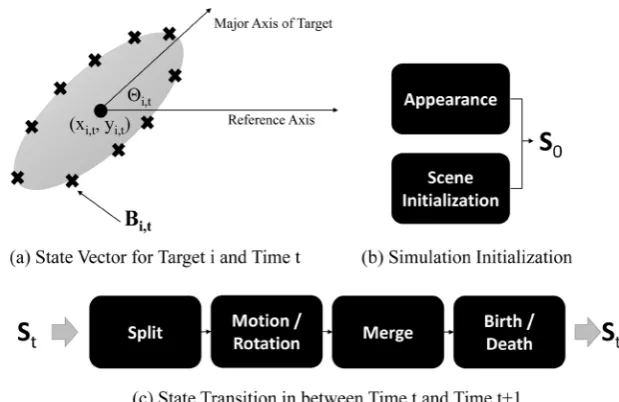
As depicted in Figure 1, the simulator for generating benchmark data is a discrete event simulator which is described by a system state St at time t and its state transition events with discrete time steps t∈

{

0,1,2, ,_T

}

. The system state St is a collection of the state vectors for each target i,

•

(

x yi t_,, i t_,

)

: a centroid coordinate of target i,

• B_i: a vector of a finite number of

(

x y,

)

-coordinates that represents the outline of target i,

• θ_{i t}_, _{: a rotation angle of the appearance of target}_i_,

and the system-level state variables of,

• n_t: the number of targets at time t, and

(5)

[image:5.595.212.522.68.269.2]

DOI: 10.4236/ojmsi.2019.71001 5 Open Journal of Modelling and Simulation Figure 1. Discrete event simulation model for generating benchmark datasets.

For time t, a synthetic image It is generated from the system state St with different imaging conditions; see details in Section 3.7. The system state St is recorded and used to generate the groudtruth of the simulated image sequence.

At time 0, the system state variables are initialized with n0 specified by a

simulator user, G0 as a n n0× 0 matrix of zeros, and the target-level state

vectors initialized randomly by the following q functions,

(

)

( )

,0 ,0 ,

,0

,

i i x y

i

x y q q q

θ

= = = _B

B

The details on the q functions are described in Section 3.1 and Section 3.2. The system state is changed from St to St+1 at time t+1 by generating a

series of the following events sequentially.

1) Consider a Split event for each of the merge events occurred at time t. When a split condition is satisfied for a merge case occurred at time t, split the merged target into target i and target j, which resets

(

Gt+1

) (

ij = Gt+1

)

ji=0. The split condition will be described in Section 3.5.

2) For each target i, Motion f and Rotation g make changes on

(

) (

)

( )

, 1 , 1 , ,

, 1 ,

, ,

i t i t i t i t

i t i t

x y f x y g

θ

+ +

+

= =

More details on f and g are described in Section 3.3.

3) Merge of target i and target j that exist at time t occurs when the merging condition described in Section 3.4 is satisfied, and it sets

(

Gt+1

) (

ij= Gt+1

)

ji =1.

4) Birth sets nt+1= +n bt t with the number of birth events bt , which increases the number of system state variables by nt. In the discrete event simulation, a birth process has been modeled by a Poisson arrival process with

(6)

DOI: 10.4236/ojmsi.2019.71001 6 Open Journal of Modelling and Simulation between two consecutive birth events follows an exponential distribution with mean 1α _{[46]. The rate parameter can be changing in time, which is denoted}

by αt. Following the approach, we sample bt from

( )

~ Poisson ,

t t

b α

where αt is the expected number of birth events occurred at time t and it can be specified by simulator users to change the level of birth events. The state vector for each of the bt born targets is initialized by the q functions,

(

)

( )

, 1 , 1 ,

, 1

,

i t i t x y

i t

i

x y q

q q θ θ + + + = = = _B B

and Gt+1 is augmented by appending bt columns and bt rows of zero values to Gt.

5) Death of target i occurs when the new centroid

(

xi t, 1+,yi t, 1+

)

is out of a pre-specified image region

[

0,m

] [ ]

× 0,n . When it occurs, it would reduce nt+1

by one and would make the removal of the corresponding target-level state vectors.

3.1. Appearance Function

q

B

The appearance function qB is a random process that generates the image coordinates on the outline of a target. By default, our simulator generates the circular outline of a target with a random radius r,

( )

(

cos ,sin

)

,

r

=

B a a

where r~

(

rmean,rsig

)

and a is a vector of equally spaced numbers in

[

0,2π

]

. When users want to customize target boundaries, users can give a set of N candidate target boundaries

{

_{B B}( )1, ( )2, ,_ _B( )N

}

. The appearance function qB randomly chooses one of the boundaries for each target with the chosen boundary index sampled from Unif 1,

(

N

)

, where Unif 1,

(

N

)

is the uniform distribution over integer numbers in 1, N.

3.2. Initial Scene Function

q

x,y

and

q

θ

At time 0, the initial scene function determines the initial location and orientation of a target by

(

)

(

)

(

)

0 ,0 ,0 ,0 1 mod

, if 0

, otherwise

, , 1 , 1

~ Unif 0,2π ,

i i

i

u n

v i u

v v

p u

i

x y m w n w d p

u θ   =_ − _ = ≠  =      = − + − + + __ − _ − _    

(7)

DOI: 10.4236/ojmsi.2019.71001 7 Open Journal of Modelling and Simulation distance d, and margin w. At time t>0_{, the initial scene function determines}

the initial location and orientation of a newly born target by

(

)

( )

(

)

, ~ Unif 0, , , ~ Unif 0, and ,0~ Unif 0,2π .

i t i t i

x m y n θ

3.3. Motion Function

f

and Rotation

g

The motion function f determines each target’s location at time step t in the simulation. Users have two choices among the Brownian motion [47] [48] [49],

(

, 1 , 1

)

(

, ,

)

0

, ~ , , ₀x .

i t i t i t i t

y

x + y + x y σ _σ

       _ _

 



and the stochastic diffusion process [50],

(

xi t, 1+,yi t, 1+

)

~

(

x yi t,, i t,

)

, ,Σ

)

where Σ is a two-by-two positive definite covariance matrix which determines the overall movement direction.

The rotation function g determines the random rotation angle of target i at time t+1_by

(

)

, 1~ Unif 0,2π .

i t

θ ₊

Once

(

xi t, 1+,yi t, 1+

)

and θi t, 1+ are sampled, the outline of target i at time t+1 is determined by the rigid body transformation of Bi,

( )

, 1

( ) (

, 1 , 1 , 1

)

, 1 , 1

cos sin

, ,

sin cos

i t i t

i i t i t

i t i t

x y

θ

+ + + + + +   +   −     B 1

where 1 is a column vector of ones which has the same size as the row size of i

B .

3.4. Merging Condition

The merge event occurs at time t in between target i and j if they spatially overlaps after the motion and the rotation applied. Since the target i’s outline would be

( )

,

( )

, , , , , , , cos sin ˆ _, sin cos

i t i t i t

i t i t

i t

i t i t

x y

θ

  _ _ =  +_ _ −       B B

the overlap of targets i and j would occur only if

(

ˆ ˆ,, ,

)

0,

H i t j t

d B B =

where d_H

(

A B,

)

is the Hausdorff distance between A and B . If the condition holds, the merge matrix Gt is updated by setting its (i, j) and (j, i) elements set to one. Once they merge, the simulator applies the same motion for the two targets so that they can move together before they split.

3.5. Split Condition

(8)

DOI: 10.4236/ojmsi.2019.71001 8 Open Journal of Modelling and Simulation probability of split is represented by a binomial distribution of the probability of split p.

3.6. Determination of the Number of Birth Events

b

t

The number of birth events at time t is determined by

( )

~ Poisson ,

t t

b α

where αt is the average number of event occurrings. The initial state of each new born target is randomly sampled from qB, qθ and qx y, .

3.7. Image and Noise Generation Function

For time t, a synthetic image It is generated from the system state St. It is a m n× grayscale image where all targets outlined by Bi t, with centroid

(

x yi t,, i t,

)

and orientation θi t, are colored black (i.e. image intensity = 0), and the remaining

background is colored white (i.e. image intensity = 255). We add the following noise components on the synthetic images to simulate different signal-to-noise ratios:

• _{Gaussian random noise:}

(

2

)

, ~ 0,

x y σ

  for each image pixel at

(

x y,

)

.

• _{Non-uniform illumination:} H_{x y}_, = f x y

₍

,

₎

for each image pixel

(

x y,

)

, and

(

,

)

f x y is the function defined by users. The output image Lt at time t follows [51]

, , , , ,

x y t =Hx y∗ x y t

L I

for each image pixel at

(

x y,

)

.

• _{Both Gaussian random noise and non-uniform illumination: The output}

image Lt at time t follows

, , , , , ,

x y t=Hx y∗ x y t+x y

L I

for each image pixel

(

x y,

)

. Gx y, and x y, are the non-uniform illumination

and Gaussian random noise generated above, respectively.

4. Performance Evaluation with the Simulator

The synthetic images generated by the simulator are used as inputs to a multi-target tracking algorithm to be tested, and the state vectors

{

S_t;t=0,1,2, ,_T

}

are used as a ground-truth to compute the performance metrics of the algorithm.

If the algorithm being tested is a tracking-by-detection algorithm [14] [15] [22], target detections are first obtained for all image frames either by obtaining target boundaries with true system state St or by choosing and running an existing target detection algorithm on simulated images. A tracking-by-detection algorithm associates the detections to target identities via one-to-one, one-to-many or many-to-one associations, which will output the data association Jt for every time frame t, which is a nt×2 matrix with the detection identifier in the

(9)

DOI: 10.4236/ojmsi.2019.71001 9 Open Journal of Modelling and Simulation state matrix Gt are used. The popular performance metric for this type of the algorithm is the accuracy of one-to-one, one-to-many (split) and many-to-one (merge) data associations in terms of the false positive (FPR) and false negative rates (FNR), which is defined by the following equations [52],

FPR FP

FP TN

=

+ (1)

FNR FN

FN TP

=

+ (2)

where FP is the number of false positives, FN is the number of false negatives, TN is the number of true negatives, and TP is the number of true positives. The false positive and false negative rates can be obtained by comparing Jt with the ground truth

{

(

x yi t,, i t,

)

,Gt

}

. Gt contains all merge and split information and

(

x yi t,, i t,

)

contains the trace of individual targets. Therefore, one

can extract all one-to-one, one-to-many and many-to-one associations by tracking

(

)

{

x yi t,, i t, ,Gt

}

, which can be directly compared with Jt for FPR and FNR. If the algorithm being tested is a filtering-based algorithm that estimates each target’s location at each time step [27] [28], its estimates can be compared with the ground-truth

{

(

x yi t,, i t,

)

}

in order to compute the popular CLEAR MOT

metrics [53], the multiple object tracking precision (MOTP) and the multiple object tracking accuracy (MOTA). The MOTP is a measure of the overall target location estimation, which is computed by

, ,

MOTP i t i t t t

d

c

=

∑

(3)

where di t, is the Euclidean distance between the location estimate and the true

target’s location

(

x yi t,, i t,

)

for target i at time t, and ct is the number of the cases that the estimates are with a certain small range from the true target’s location, at time t. The MOTA is

(

)

MOTA 1 t t t t

t t

FN FP MM g

+ +

= −

∑

(4)

where FNt, FPt, and MMt are the number of false negatives, false positives, and missed matches respectively for t, and gt is the total number of ground-truth targets at time t.

5. Demonstration

In this section, we demonstrate the use of our simulator in generating bench-mark data and evaluating multitarget tracking algorithms with the benchbench-mark data.

5.1. Simulate Benchmark Datasets with Our Simulator

(10)

DOI: 10.4236/ojmsi.2019.71001 10 Open Journal of Modelling and Simulation following input parameters, total number of image frames: T; initial number of targets: n0; target appearance: circle of a radius with mean rmean and standard deviation rsig; spatial distance in between targets at the first frame: d; image size:

2m n×2 ; temporal change in target locations: σx along x-direction and σy along y-direction; average number of birth events per time: αt; image noise: white noise with noise variance _σ2

 and non-uniform illumination with f x y

(

,

)

;

probability of split: p.

Figure 2 shows example images generated with T =10, n0=5, rmean=1,

0.1

sig

r = _, d=6_, m=13_, n=13_, σ_x=σ_y =0.5_, α =t 1, σ = 0.09,

(

,

)

2₂ 2₂

1

x y

f x y

x y

+ =

− − , and p=0.8.

5.2. Testing and Evaluating Tracking-by-Detection Algorithms

We demonstrate the use of our simulator to evaluate the multiway data association [22] and the linear programming approach [21]. For the evaluation, we designed the experiment by a 23_{factorial design of three variables, the initial} distance in between two closest targets (d), target movement speed (σx and

y

σ ), and target birth rate (αt), as seen in Table 1. We fixed the other simulation inputs to T =10_, n₀=₁₀, rmean =1, rsig =0.1, m=13, n=13, σ = 0.09,

(

,

)

1

f x y = , and p=0.8.

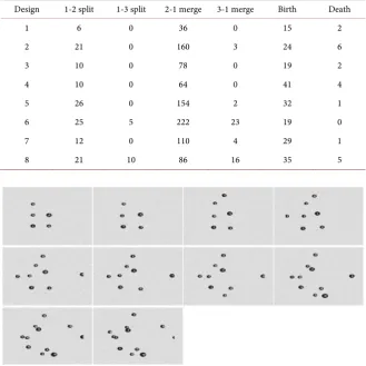
For each design, we performed ten simulation runs with the same design va-riables for replicated experiments to reduce any random effects on the evalua-tion outcomes. For each simulaevalua-tion run, we recorded the numbers of merging events, splitting events, target births, and target deaths occurred during the si-mulation run. Table 2 shows the average numbers for ten replicated experi-ments for each design. As observed in Table 2, the complexity of the simulated tracking scenarios change as we vary simulation inputs. For example, when we decrease the distance d and/or increase the temporal variation of target location,

x

σ and σy, more merging and splitting events occur. With the increased birth rate αt, more birth events occur.

[image:10.595.211.538.570.731.2]

For each replication, we input the images generated by our simulator ten

Table 1. Design of experiments for evaluating tracking-by-detection algorithms.

d σx, σy αt

(11)

[image:11.595.208.539.98.436.2]

DOI: 10.4236/ojmsi.2019.71001 11 Open Journal of Modelling and Simulation Table 2. Average number of target split, merge, birth and death events occurred per an experimental run.

Design 1-2 split 1-3 split 2-1 merge 3-1 merge Birth Death

1 6 0 36 0 15 2

2 21 0 160 3 24 6

3 10 0 78 0 19 2

4 10 0 64 0 41 4

5 26 0 154 2 32 1

6 25 5 222 23 19 0

7 12 0 110 4 29 1

8 21 10 86 16 35 5

Figure 2. Simulated video frame.

[image:11.595.209.539.102.432.2]

(12)

[image:12.595.208.537.111.601.2]

DOI: 10.4236/ojmsi.2019.71001 12 Open Journal of Modelling and Simulation Table 3. The average false positive rate (FPR) and false negative rate (FNR) for the

mul-tiway data association [22] and the linear programming approach [21] over ten replicated

simulations for Designs 1 through 4.

Multiway data association Linear programming approach

Design 1 FPR FNR FPR FNR

1-to-1 0.0202 0.0041 0.0202 0.0041 1-to-2 0.1111 0.0000 0.1111 0.0000 2-to-1 0.0000 0.0000 0.0000 0.0000 1-to-3 0.0000 0.0000 0.0000 0.0000 3-to-1 0.0000 0.0000 0.0000 0.0000 Birth 0.0000 0.0000 0.0000 0.0000 Death 0.0000 0.0000 0.0000 0.0000

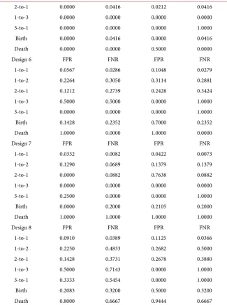
Table 4. The average false positive rate (FPR) and false negative rate (FNR) for the

mul-tiway data association [22] and the linear programming approach [21] over ten replicated

simulations for Designs 5 through 8.

Multiway data association Linear programming approach

[image:12.595.211.538.659.719.2]

(13)

DOI: 10.4236/ojmsi.2019.71001 13 Open Journal of Modelling and Simulation

Continued

2-to-1 0.0000 0.0416 0.0212 0.0416 1-to-3 0.0000 0.0000 0.0000 0.0000 3-to-1 0.0000 0.0000 0.0000 1.0000 Birth 0.0000 0.0416 0.0000 0.0416 Death 0.0000 0.0000 0.5000 0.0000

splitting evets. Overall, the multiway data association [22] performed better than the linear programming approach [21] in detecting all merging and splitting events.

Evaluating Filtering-Based Algorithms

In this section, we use our simulator to evaluate a simple Kalman filtering-based algorithm [1] [54] [55] to see how it performs with different levels of image noises and different numbers of targets. We performed a 22_{factorial design of} two factors n0 and σ as described in Table 5, while controlling the other

factors to T =10_, rmean=1, rsig=0.1, m=13, n=13, σ =x 0.15, σy =0.15,

5

d= _, f x y

(

,

)

=1, α =t 0.3 and p=0.8.

[image:13.595.212.538.85.522.2]

(14)

[image:14.595.210.540.89.174.2]

DOI: 10.4236/ojmsi.2019.71001 14 Open Journal of Modelling and Simulation Table 5. Design of experiments for evaluating a Kalman filtering-based algorithm.

0

n σ_

Design 1 5 0

Design 2 5 0.5

Design 3 20 0

[image:14.595.210.540.205.433.2]

Design 4 20 0.5

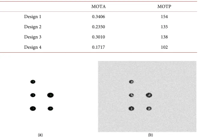
Table 6. Average MOTA and MOTP metrics.

MOTA MOTP

Design 1 0.3406 154

Design 2 0.2350 135

Design 3 0.3010 138

Design 4 0.1717 102

Figure 3. Simulated video frame. (a) Design 1; (b) Design 2.

For each experiment run, the Kalman-filtering-based algorithm first read in simulated images, detects each target in the scene and finally estimates each target’s position with the Kalman filter. We computed the MOTP and MOTA metrics in order to evaluate the accuracy of the estimation. Table 6 summarizes the average MOTP and MOTA metrics over ten simulation runs for each design, where high values implies higher accuracy for both of the metrics [53]. The performance degradation of the algorithm was significant with the increased level of noises, but the effect of the number of targets on the performance was not significant.

6. Conclusion

(15)

DOI: 10.4236/ojmsi.2019.71001 15 Open Journal of Modelling and Simulation evaluate multitarget tracking algorithms. We demonstrated the use of the proposed simulation model to evaluate two tracking-by-detection algorithms and one filtering-based algorithm. In addition, the simulator can generate new public benchmark datasets with high-degree of interactions and complexity with ease from the user’s inputs.

Acknowledgements

This project was partially supported by the National Science Foundation with grant no NSF-CMMI-1334012, the Air Force Office of Scientific Research with grant no FA9550-13-1-0075, and the Florida State University Council on Research and Creativity Planning Grant 036656.

Conflicts of Interest

The authors declare no conflicts of interest regarding the publication of this pa-per.

References

[1] Popoli, R. and Blackman, S.S. (1999) Design and Analysis of Modern Tracking

Sys-tems. Artech House, Norwood, MA.

[2] Yilmaz, A., Javed, O. and Shah, M. (2006) Object Tracking: A Survey. ACM

Com-puting Survey, 38, 1-45.https://doi.org/10.1145/1177352.1177355

[3] Skolnik, M.I. (1990) Radar Handbook. McGraw-Hill, New York City, NY.

[4] Stone, L.D., Streit, R.L., Corwin, T.L. and Bell, K.L. (2013) Bayesian Multiple Target

Tracking. Artech House, Norwood, MA.

[5] Bar-Shalom, Y. (1987) Tracking and Data Association. Academic Press

Profession-al, Inc.

[6] Blackman, S.S. (1986) Multiple-Target Tracking with Radar Applications. Artech

House, Inc., Dedham, MA.

[7] Mahler, R.P.S. (2007) Statistical Multisource-Multitarget Information Fusion.

Ar-tech House, Norwood, MA.

[8] Lane, D.M., Chantler, M.J. and Dai, D.Y. (1998) Robust Tracking of Multiple

Ob-jects in Sector-Scan Sonar Image Sequences Using Optical Flow Motion Estimation.

IEEE Journal Oceanic Engineering, 23, 31-46.

https://doi.org/10.1109/48.659448

[9] Kocak, D.M., da Vitoria Lobo, N. and Widder, E. (1999) A Computer Vision

Tech-niques for Quantifying, Tracking, and Identifying Bioluminescent Plankton. IEEE

Journal Oceanic Engineering, 24, 81-95.https://doi.org/10.1109/48.740157

[10] Durrant-Whyte, H. and Bailey, T. (2006) Simultaneous Localization and Mapping:

Part I. IEEE Robotics and Automation Magazine, 13, 99-110.

https://doi.org/10.1109/MRA.2006.1638022

[11] Bailey, T. and Durrant-Whyte, H. (2006) Simultaneous Localization and Mapping

(SLAM): Part II. IEEE Robotics and Automation Magazine, 13, 108-117.

https://doi.org/10.1109/MRA.2006.1678144

[12] Spagnolini, U. and Rampa, V. (1999) Multitarget Detection/Tracking for

(16)

Transac-DOI: 10.4236/ojmsi.2019.71001 16 Open Journal of Modelling and Simulation tions on Geoscience and Remote Sensing, 37, 383-394.

https://doi.org/10.1109/36.739074

[13] Sethi, I.K. and Jain, R. (1987) Finding Trajectories of Feature Points in a Monocular

Image Sequence. IEEE Transactions on Pattern Analysis and Machine Intelligence,

9, 56-73.

[14] Veenman, C.J., Reinders, M.J.T. and Backer, E. (2001) Resolving Motion

Corres-pondence for Densely Moving Points. IEEE Transactions on Pattern Analysis and

Machine Intelligence, 23, 54-72.https://doi.org/10.1109/34.899946

[15] Pirsiavash, H., Ramanan, D. and Fowlkes, C.C. (2011) Globally-Optimal Greedy

Algorithms for Tracking a Variable Number of Objects. IEEE Conference on

Com-puter Vision and Pattern Recognition, Colorado Springs, 20-25 June 2011, 1201-1208.

[16] Jiang, H., Fels, S. and Little, J.J. (2007) A Linear Programming Approach for

Mul-tiple Object Tracking. IEEE Conference on Computer Vision and Pattern

Recogni-tion, Minneapolis, 17-22 June 2007, 1-8.

[17] Zhang, L., Li, Y. and Nevatia, R. (2008) Global Data Association for Multi-Object

Tracking Using Network Flows. IEEE Conference on Computer Vision and Pattern

Recognition, Anchorage, 23-28 June 2008, 1-8.

[18] Jaqaman, K., Loerke, D., Mettlen, M., Kuwata, H., Grinstein, S., Schmid, S.L. and

Danuser, G.R. (2008) Single-Particle Tracking in Live-Cell Time-Lapse Sequences.

Nature Methods, 5, 695-702.https://doi.org/10.1038/nmeth.1237

[19] Serge, A., Bertaux, N., Rigneault, H. and Marguet, D. (2008) Dynamic

Mul-tiple-Target Tracing to Probe Spatiotemporal Cartography of Cell Membranes.

Na-ture Methods, 5, 687-694.https://doi.org/10.1038/nmeth.1233

[20] Choi, W. and Savarese, S. (2012) A Unified Framework for Multi-Target Tracking

and Collective Activity Recognition. European Conference on Computer Vision,

Florence, 7-13 October 2012, 215-230.

[21] Henriques, J.F., Caseiro, R. and Batista, J. (2011) Globally Optimal Solution to

Mul-ti-Object Tracking with Merged Measurements. IEEE International Conference on

Computer Vision, Barcelona, 6-13 November 2011, 2470-2477.

[22] Park, C., Woehl, T.J., Evans, J.E. and Browning, N.D. (2014) Minimum Cost

Mul-ti-Way Data Association for Optimizing Multitarget Tracking of Interacting

Ob-jects. IEEE Transactions on Pattern Analysis and Machine Intelligence, 37, 611-624.

https://doi.org/10.1109/TPAMI.2014.2346202

[23] Broida, T.J. and Chellappa, R. (1986) Estimation of Object Motion Parameters from

Noisy Images. IEEE Transactions on Pattern Analysis and Machine Intelligence, 8,

90-99.

[24] Beymer, D. and Konolige, K. (1999) Real-Time Tracking of Multiple People Using

Continuous Detection.

[25] Rosales, R. and Sclaroff, S. (1999) 3D Trajectory Recovery for Tracking Multiple

Objects and Trajectory Guided Recognition of Actions. IEEE Conference on

Com-puter Vision and Pattern Recognition, Colorado, 23 June 1999, 117-123.

[26] Tanizaki, H. (1996) Nonlinear Filters: Estimation and Applications. Springer, New

York City, 400.

[27] Khan, Z., Balch, T. and Dellaert, F. (2004) An MCMC-Based Particle Filter for

Tracking Multiple Interacting Targets. European Conference on Computer Vision,

Prague, 11-14 May 2004, 279-290.

(17)

Filtering. IEEE Transactions on Aerospace Electronics System, 38, 791-812.

https://doi.org/10.1109/TAES.2002.1039400

[29] Genovesio, A. and Olivo-Marin, J.-C. (2004) Split and Merge Data Association

Fil-ter for Dense Multi-Target Tracking. International Conference on Pattern

Recogni-tion,4, 677-680.

[30] Khan, Z., Balch, T. and Dellaert, F. (2005) Multi-Target Tracking with Split and

Merged Measurements. IEEE Conference on Computer Vision and Pattern

Recog-nition, San Diego, 20-26 June 2005, Vol. 1, 605-610.

[31] Khan, Z., Balch, T. and Dellaert, F. (2006) MCMC Data Association and Sparse

Factorization Updating for Real Time Multi-Target Tracking with Merged and

Multiple Measurements. IEEE Transactions on Pattern Analysis and Machine

Intel-ligence, 28, 1960-1972.https://doi.org/10.1109/TPAMI.2006.247

[32] Storlie, C.B., Lee, T.C.M., Hannig, J. and Nychka, D. (2009) Tracking of Multiple

Merging and Splitting Targets: A Statistical Perspective. Statistica Sinica, 19, 1-52.

[33] Yang, B. and Nevatia, R. (2012) Multi-Target Tracking by Online Learning of

Non-Linear Motion Patterns and Robust Appearance Models. IEEE Conference on

Computer Vision and Pattern Recognition, Providence, 16-21 June 2012, 1918-1925.

[34] Alahi, A., Jacques, L., Boursier, Y. and Vandergheynst, P. (2011) Sparsity Driven

People Localization with a Heterogeneous Network of Cameras. Journal of

Mathe-matical Imaging and Vision, 41, 39-58.https://doi.org/10.1007/s10851-010-0258-7

[35] BIWI Walking Pedestrians Dataset Computer Vision Laboratory-ETH, 2009.

[36] Pellegrini, S., Ess, A., Schindler, K. and Van Gool, L. (2009) You’ll Never Walk

Alone: Modeling Social Behavior for Multi-Target Tracking. International

Confe-rence on Computer Vision, Kyoto, 27 September-4 October 2009, 261-268.

[37] Andriluka, M., Roth, S. and Schiele, B. (2010) Monocular 3D Pose Estimation and

Tracking by Detection. IEEE Conference on Computer Vision and Pattern

Recogni-tion, San Francisco, 13-18 June 2010, 623-630.

[38] Yang, B. and Nevatia, R. (2012) An Online Learned CRF Model for Multi-Target

Tracking. IEEE Conference on Computer Vision and Pattern Recognition,

Provi-dence, 16-21 June 2012, 2034-2041.

[39] Milan, A., Roth, S. and Schindler, K. (2014) Continuous Energy Minimization for

Multitarget Tracking. IEEE Transactions on Pattern Analysis and Machine

Intelli-gence, 36, 58-72.https://doi.org/10.1109/TPAMI.2013.103

[40] Milan, A., Schindler, K. and Roth, S. (2013) Challenges of Ground Truth Evaluation

of Multi-Target Tracking. IEEE Conference on Computer Vision and Pattern

Rec-ognition Workshops, Portland, 23-28 June 2013, 735-742.

[41] Pedestrian Mobile Scene Analysis Computer Vision Laboratory-ETH, 2009.

[42] Ess, A., Leibe, B. and Van Gool, L. (2007) Depth and Appearance for Mobile Scene

Analysis. International Conference on Computer Vision, Rio de Janeiro, 14-20

Oc-tober 2007, 1-8.

[43] Benfold, B. and Reid, I. (2011) Stable Multi-Target Tracking in Real-Time

Surveil-lance Video. IEEE Conference on Computer Vision and Pattern Recognition,

Colo-rado, 20-25 June 2011, 3457-3464.

[44] Nannuru, S., Coates, M. and Mahler, R. (2013) Computationally-Tractable

Ap-proximate Probability Hypothesis Density and Cardinalized Probability Hypothesis

Density Filters for Superpositional Sensors. IEEE Journal Selective Topics in Signal

(18)

[45] Hoseinnezhad, R., Vo, B.-N. and Vo, B.-T. (2013) Visual Tracking in Background

Subtracted Image Sequences via Multi-Bernoulli Filtering. IEEE Transactions on

Pattern Analysis and Machine Intelligence, 61, 392-397.

[46] Pinsky, M. and Karlin, S. (2010) An Introduction to Stochastic Modeling. Academic

Press, Waltham.

[47] Hida, T. (1980) Brownian Motion. Springer, New York.

[48] Karatzas, I. (1991) Brownian Motion and Stochastic Calculus. Springer, New York.

[49] Revuz, D. and Yor, M. (1999) Continuous Martingales and Brownian Motion.

Springer, New York.

[50] Bibbona, E., Panfilo, G. and Tavella, P. (2008) The Ornstein-Uhlenbeck Process as a

Model of a Low Pass Filtered White Noise. Metrologia, 45, 117.

https://doi.org/10.1088/0026-1394/45/6/S17

[51] Matsushita, Y., Nishino, K., Ikeuchi, K. and Sakauchi, M. (2004) Illumination

Nor-malization with Time-Dependent Intrinsic Images for Video Surveillance. IEEE

Transactions on Pattern Analysis and Machine Intelligence, 26, 1336-1347.

https://doi.org/10.1109/TPAMI.2004.86

[52] Sheskin, D.J. (2003) Handbook of Parametric and Nonparametric Statistical

Proce-dures. CRC Press, Boca Raton.

[53] Keni, B. and Rainer, S. (2008) Evaluating Multiple Object Tracking Performance:

The CLEAR MOT Metrics. EURASIP Journal in Image and Video Processing, 2008,

Article ID: 246309.

[54] Brown, R.G., Hwang, P.Y.C., et al. (1992) Introduction to Random Signals and

Ap-plied Kalman Filtering. Wiley, Hoboken.

[55] Kim, P. and Huh, L. (2011) Kalman Filter for Beginners: With MATLAB Examples.

CreateSpace, Seattle.

Nomenclature

ETH: Eidgenssische Technische Hochschule FN: False Negative

FNR: False Negative Rate FP: False Positive FPR: False Positive Rate

MCMC: Markov Chain Monte Carlo MOT: Multiple Object Tracking

MOTA: Multiple Object Tracking Accuracy MOTP: Multiple Object Tracking Precision

PETS: Performance Evaluation of Tracking and Surveillance TN: True Negative

TP: True Positive