Constant-Envelope Multi-Level Chirp Modulation: Properties, Receivers, and Performance

(1)

Electronic Thesis and Dissertation Repository

2-16-2016 12:00 AM

Constant-Envelope Multi-Level Chirp Modulation: Properties,

Receivers, and Performance

Mohammad A. Alsharef The University of Western Ontario Supervisor

Dr. Rao, Raveendra

The University of Western Ontario

Graduate Program in Electrical and Computer Engineering

A thesis submitted in partial fulfillment of the requirements for the degree in Doctor of Philosophy

Follow this and additional works at: https://ir.lib.uwo.ca/etd

Part of the Systems and Communications Commons

Recommended Citation Recommended Citation

Alsharef, Mohammad A., "Constant-Envelope Multi-Level Chirp Modulation: Properties, Receivers, and Performance" (2016). Electronic Thesis and Dissertation Repository. 3534.

https://ir.lib.uwo.ca/etd/3534

This Dissertation/Thesis is brought to you for free and open access by Scholarship@Western. It has been accepted for inclusion in Electronic Thesis and Dissertation Repository by an authorized administrator of

(2)

Constant envelope multi-level chirp modulations, with and without memory, are

con-sidered for data transmission. Specifically, three subclasses referred to as

symbol-by-symbol multi-level chirp modulation, full-response phase-continuous multi-level chirp

modulation and full-response multi-mode phase-continuous multi-level chirp

modula-tion are considered. These modulated signals are described, illustrated, and examined

for their properties. The ability of these signals to operate over AWGN is assessed

using upper bounds on minimum Euclidean distance as a function of modulation

pa-rameters. Coherent and non-coherent detection of multi-level chirp signals in AWGN

are considered and optimum and sub-optimum receiver structures are derived. The

performance of these receivers have been assessed using upper and lower bounds as

a function of SNR, modulation parameters, modulation levels, decision symbol

lo-cations, and observation length of receiver. Optimum multi-level chirp modulations

have been determined using numerical minimization of symbol error rate.

Closed-form expressions are derived for estimating the perClosed-formance of multi-level chirp

sig-nals over several practical fading channels. Finally, spectral characteristics of digital

chirp signals are presented and illustrated.

(3)

All praise be to Allah Almighty, the most merciful and most compassionate, for

bestowing upon me His countless bounties and for providing me the opportunity to

carry out my PhD degree. Without his guidance and blessings, nothing is possible.

I would like to express my sincerest gratitude and deep appreciation to my

su-pervisor Dr.Raveendra K. Rao who has supported me throughout my PhD study at

the University of Western Ontario. His extensive knowledge in the field of

commu-nications, encouragement, guidance, and constructive criticism have been valuable

resources. Also, I would like to thank the examination committee members for their

valuable remarks and considerable recommendations.

I am extremely grateful to my parents and my family for their support and

encouragement over the years. The role of my parents in my upbringing and their

prayers have played a major role in what I am today. I wish that I can compensate

them for the past years.

I can never thank enough all my friends and my colleagues with whom I have the

pleasure to work with in the same research lab for the unforgettable times we spent

together. I have benefited from discussing diverse subjects related to the research

and life in general.

Last but not least, I would like to thank Taif University for supporting me in

completing my PhD study. Also, I thank the Ministry of Education in Saudi Arabia

and the Saudi Cultural Bureau in Canada for their support.

(4)

Abstract . . . ii

Acknowledgements . . . iii

List of tables . . . vii

List of figures . . . ix

Acronyms . . . xiii

1 Introduction . . . 1

1.1 Introduction to Communications . . . 1

1.2 Wireless Communications . . . 1

1.3 Digital Communication System . . . 2

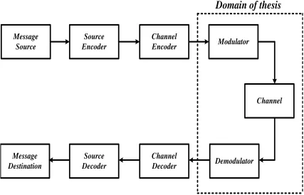
1.4 Simplified Model of Digital Communication System . . . 4

1.5 Literature Survey and Motivation . . . 7

1.6 Thesis Objectives . . . 11

1.7 Thesis Organization . . . 12

2 Memoryless Constant-Envelope Multi-Level Chirp Modulation: Co-herent and Non-CoCo-herent Detection . . . 14

2.1 Introduction . . . 14

2.2 Constant Envelope Multi-Level Chirp Modulated Signals . . . 15

2.2.1 2-level (2-ary) or Binary Chirp Modulation . . . 17

2.2.2 4-level (4-ary) or Quaternary Chirp Modulated Signals . . . . 18

2.3 Minimum Euclidean Distance Properties . . . 19

2.4 Coherent Detection and Performance of Multi-level (M-ary) Chirp Sig-nals . . . 27

2.4.1 Coherent Detection . . . 27

2.4.2 Error Rate Performance . . . 31

2.4.3 Numerical Results . . . 32

2.5 Non-Coherent Detection and Performance of Multi-level (M-ary) Chirp Signals . . . 41

2.5.1 Non-Coherent Detection . . . 41

2.5.2 Error Rate Analysis . . . 43

2.5.3 Numerical Results . . . 46

(5)

Signals and Distance Properties . . . 54

3.2 M-level Continuous Phase Chirp Modulation (M-CPCM) Signals . . 55

3.3 Minimum Euclidean Distance Properties . . . 59

3.4 Bounds on The Minimum Euclidean Distance . . . 64

3.5 Numerical Results and Discussion . . . 65

3.6 Conclusions . . . 76

4 Detection and Performance of M-CPCM in AWGN Channel . . . 77

4.2 Coherent Detection of M-CPCM . . . 77

4.2.1 Optimum Coherent Receiver . . . 78

4.2.2 Symbol Error Probability Analysis . . . 81

4.2.3 Numerical Results and Discussion . . . 88

4.3 Non-coherent Detection of M-CPCM in AWGN . . . 98

4.3.1 Optimum Non-coherent Receiver . . . 98

4.3.2 Symbol Error Probability Analysis . . . 100

4.3.3 Numerical Results and Discussion . . . 105

5 Multi-Mode Multi-Level Continuous Phase Chirp Modulation: Co-herent Detection . . . 113

5.2 Multi-modeM-CPCM Signals . . . 113

5.3 Optimum Coherent Receiver and Performance Analysis . . . 117

6 Memoryless Multi-level Chirp Modulation over Fading Channels . 128 6.1 Introduction . . . 128

6.2 Fading Channel Models . . . 128

6.2.1 Rayleigh Fading Channel . . . 129

6.2.2 Nakagami-m Fading Channel . . . 129

6.2.3 Generalized-K Fading and Shadowing Channel . . . 130

6.3 Average Symbol Error Rate Expressions for Memoryless M-CPCM . 131 6.3.1 Rayleigh Fading Channel . . . 131

6.3.2 Performance analysis over Nakagami-m Fading Channel . . . . 132

6.3.3 Generalized-K Fading and Shadowing Channel . . . 133

(6)

7 Spectral Characteristics of M-CPCM Signals . . . 142

7.2 Spectral Calculation Methods . . . 142

7.3 Spectra of M-CPCM . . . 143

7.4 Spectra of Mono-modeM-CPCM Signals . . . 146

8 Conclusion . . . 151

8.2 Summary of Contributions . . . 151

8.3 Suggestions for Future Work . . . 154

References . . . 155

Appendices A Squared Euclidean Distance for M-Level Chirp Signals . . . 160

B Complex Correlation for M-Level Chirp Signals . . . 164

Curriculum Vitae . . . 166

(7)

2.1 (q, w) maximizing d2_min for M-level chirp modulated signals . . . 21

2.2 d2_min forM-level chirp modulated signals, M-PSK, andM-FSK

mod-ulations . . . 22

2.3 Optimum modulation parameters (qopt, wopt) for M =2,4,8 and

16-chirp systems . . . 35

2.4 Bit Error Rate Comparison of Optimum 2-level chirp, BPSK and

bi-nary FSK . . . 36

2.5 Symbol Error Rate Performance of Optimum 4-level chirp, QPSK and

4-FSK . . . 39

2.6 Symbol Error Rate Performance of Optimum 8-level chirp, 8-PSK and

8-FSK . . . 39

2.7 Symbol Error Rate Performance of Optimum 16-level chirp, 16-PSK

and 16-FSK . . . 40

2.8 Symbol Error Rate Performance of Optimum Non-coherent 2-level chirp,

2-DPSK and 2-FSK . . . 50

3.1 (q, w) maximizing d2_B,M for M-CPCM . . . 66

3.2 h maximizing d2_B,M for M-CPFSK . . . 68

3.3 Optimum modulation parameters maximizingd2_n and Gn for 2-CPCM

and 2-CPFSK . . . 70

4.1 Optimum (q, w) 2-CPCM systems as a function of observation intervals

n and SNR (E_b/N₀) . . . 88

n and SNR (E_b/N0) . . . 89

n and SNR (E_b/N₀) . . . 89

(8)

4.4 Error probabilities of 2-CPCM, BPSK, and 2-FSK atE_b/N₀=6, 8, and

10 dB . . . 91

4.5 Probability of error comparison of 2-CPCM and 2-CPFSK . . . 92

4.6 Error probabilities of 4-CPCM and QPSK at E_b/N0=6, 8, and 10 dB 94 4.7 Probability of error comparison of 4-CPCM and 4-CPFSK . . . 95

4.8 Error probabilities of 8-CPCM and 8-PSK . . . 96

4.9 Probability of error comparison of 8-CPCM and 8-CPFSK . . . 97

4.10 Optimum (q, w) sets for non-coherent 2-CPCM system as a function of n and . . . 106

4.13 Error probability of 2-CPCM and 2-CPFSK at SNR= 6, 8, and 10 dB 109 4.14 Error probabilities for non-coherent 4-CPCM and 4-CPFSK at Eb N₀ = 6,8, and 10 dB . . . 111

5.1 Optimum dual-mode 2-CPCM modulation parameter sets . . . 121

5.4 Error probabilities of dual-mode and mono-mode 2-CPCM systems at E_b N₀= 6, 8, 10 dB . . . 123

5.5 Error probabilities of dual-mode and mono-mode 4-CPCM at Eb N0= 6, 8, 10 dB . . . 125

5.6 Error probabilities of dual-mode and mono-mode 8-CPCM at Eb N₀= 6, 8, 10 dB . . . 127

(9)

1.1 Model of point-to-point digital communication system . . . 3

1.2 Partial Block Diagram of DCS . . . 5

2.1 Schematic block diagram of M-level (M = 2k) chirp modulator . . . . 16

2.2 Phase (a) and frequency (b) as a function of time for arbitrary binary chirp signal . . . 17

2.3 Up-chirp (a) and down-chirp (b) Signals . . . 18

2.4 4-level chirp modulated signals as a function of time . . . 19

2.5 Contour plot of d2_min for 2-level chirp signals . . . 23

2.6 Surface plot of d2_min for 2-level chirp signals . . . 23

2.17 Optimum coherent receiver for M-level chirp modulation . . . 30

2.18 log₁₀(P₂(✏)/min_{P₂(✏)_}) contour plot for coherent 2-level chirp re-ceiver at 6 dB SNR . . . 33

2.19 log₁₀(P₄(✏)/min_{P₄(✏)_}) contour plot for coherent 4-level chirp re-ceiver at 6 dB SNR . . . 34

2.20 log₁₀(P8(✏)/min{P8(✏)}) contour plot for coherent 8-level chirp re-ceiver at 6 dB SNR . . . 34

2.21 log₁₀(P₁₆(✏)/min_{P₁₆(✏)_}) contour plot for coherent 16-level chirp re-ceiver at 6 dB SNR . . . 35

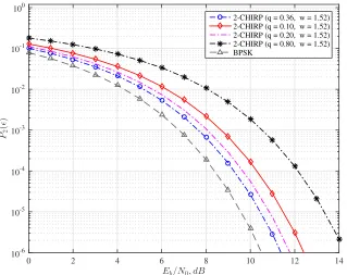
2.22 Error probability performance of optimum coherent binary chirp sys-tem (q= 0.36, w = 1.52) . . . 36

2.23 Error probability performance of coherent binary chirp system as a function ofw, for a fixed value of q= 0.36 . . . 37

2.24 Error probability performance of coherent binary chirp system as a function ofq, for a fixed value of w= 1.52 . . . 38

(10)

2.25 Error probability performance of coherent 4-level optimum chirp

sys-tem (q= 0.4, w = 2.4) . . . 38

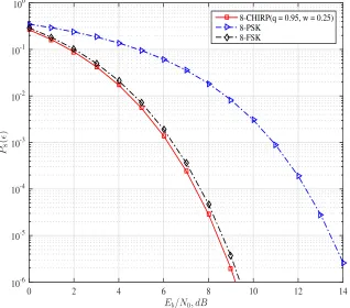
2.26 Error probability performance of coherent 8-level optimum chirp sys-tem (q= 0.95, w = 0.25) . . . 40

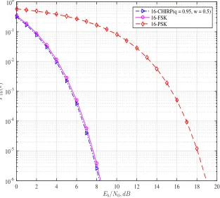
2.27 Error probability performance of coherent 16-level optimum chirp sys-tem (q= 0.95, w = 0.5) . . . 41

2.28 Optimum non-coherent receiver for M-level chirp signals . . . 43

2.29 log₁₀(P₂(✏)/min_{P₂(✏)_}) contour plot for non-coherent 2-level chirp receiver at 6 dB SNR . . . 46

2.30 log₁₀(P4(✏)/min{P4(✏)}) contour plot for non-coherent 4-level chirp receiver at 6 dB SNR . . . 47

2.31 log₁₀(P₈(✏)/min{P₈(✏)}) contour plot for non-coherent 8-level chirp receiver at 6 dB SNR . . . 47

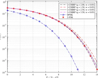
2.32 Error probability performance of optimum (q = 2.00, w = 0.05) non-coherent binary chirp system . . . 48

2.33 Error probability performance of non-coherent binary chirp system as a function ofw, for a fixed value of q = 2.00 . . . 49

2.34 Error probability performance of non-coherent binary chirp system as a function ofq, for a fixed value of w= 0.05 . . . 49

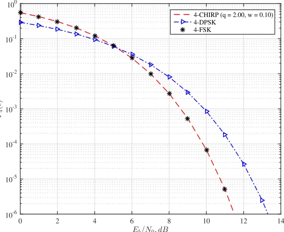
2.35 Error probability performance of (q = 2.00, w = 0.10) non-coherent 4-ary chirp system . . . 50

2.36 Error probability performance of (q = 3.00, w = 0.10) non-coherent 8-ary chirp system . . . 51

3.1 Phase tree for 2-CPCM signal . . . 57

3.2 Phase tree for 4-CPCM signal . . . 58

3.3 Phase trellis for 2-CPCM signal withq = 1₂ and arbitrary w . . . 59

3.4 Phase tree for 2-CPCM signal with merging point . . . 65

3.5 Phase tree for 4-CPCM signal with merging points . . . 66

3.6 Surface plot of d2_B,2 as a function of q and wfor 2-CPCM . . . 67

3.9 d2_B forM-CPFSK for (M=2, 4, 8) . . . 69

3.10 Surface plots of d2_n as a function of q and w for (a) n = 2, (b) n = 3, and (c)n = 4 for 2-CPCM . . . 71

3.13 Squared Euclidean distance d2₂ as a function of w for 2-CPCM with (q= 0.2,0.3,0.4,0.5,0.8) . . . 74

(11)

(w= 1.6,1.9,1,2.2,3) . . . 74

3.15 Contour plots ofGn(q, w) for 2-CPCM signals for (a)n = 2, (b)n = 3,

and (c)n = 4 . . . 75

4.1 Optimum coherent M-CPCM receiver . . . 82

4.2 High-SNR sub-optimum coherentM-CPCM receiver . . . 84

4.3 Error probability performance of optimum 2-CPCM systems for n =

2,3,4 and 5 . . . 90

4.4 Error probability performance of optimum 2-CPCM systems as a

func-tion n at Eb

N0= 6, 8, 10 and 12 dB . . . 91

4.5 Error probability performance of 2-CPFSK (h= 0.715) for n = 2,3,4

and 5 . . . 92

4.6 Symbol error probability performance of optimum 4-CPCM systems

for n= 2,3,4 and 5 . . . 93

4.7 Error probability performance of optimum 4-CPCM systems as a

func-tion of n at _NEb

0= 6, 8, 10, and 12 dB . . . 94

4.8 Error probability performance of 4-CPFSK for n= 2,3,4 and 5 . . . 95

4.9 Symbol error probability performance of 8-CPCM forn = 2 and 3 and

8-PSK . . . 96

4.10 Symbol error probability performance of 8-CPFSK for n= 2 and 3 . . 97

4.11 Optimum non-coherent M-CPCM receiver . . . 101

4.12 Sub-ptimum non-coherent M-CPCM receiver . . . 103

4.13 Error probability performance of non-coherent 2-CPCM for n = 3 and 5108

4.14 Error probability performance of non-coherent 2-CPFSK forn = 3 and

5) . . . 109 4.15 Error probability performance of non-coherent 4-CPCM systems for

n= 3 and 5 . . . 110

4.16 Error probability performance of non-coherent 4-CPFSK h= 0.715 for

n= 3 and 5 . . . 111

5.1 Phase (a) and instantaneous frequency (b) for a dual-mode 2-CPCM

system . . . 115

5.2 Phase tree for dual-mode 2-CPCM system . . . 116

5.3 Optimum coherent multi-mode M-CPCM receiver . . . 118

5.4 Error probability performance of dual-mode 2-CPCM for n = 2,3,4

and 5 and BPSK . . . 122

5.5 Error probability performance of dual-mode and mono-mode 2-CPCM

for n= 4 and 5 . . . 123

5.6 Error probability performance of dual-mode 4-CPCM forn = 2,3, and 4124

for n= 3 and 4 . . . 125

(12)

5.8 Error probability performance of dual-mode 8-CPCM for n = 2 and 3 126

for (n = 2 and 3) . . . 126

6.1 Average symbol error rate performance of optimum 2-level chirp system (q= 0.36, w = 1.52) over Rayleigh fading channel . . . 134

6.2 Average symbol error rate performance of 2-level chirp system over Rayleigh fading channel as a function ofw= 1.52(optimum), 1, 4, 7, for a fixed value of q= 0.36 . . . 134

6.3 Average symbol error rate performance of 2-level chirp system over Rayleigh fading channel as a function ofq=0.36 (optimum), 0.1, 0.2, 0.9, for a fixed value ofw= 1.52 . . . 135

6.4 Average symbol error rate performance of 4-level chirp system (q = 0.40, w = 2.40) over Rayleigh fading channel . . . 136

6.5 Average symbol error rate performance of 8-level chirp system (q = 0.95, w = 0.25) over Rayleigh fading channel . . . 136

6.6 Average symbol error rate performance of 2-level chirp system (q = 0.36, w = 1.52) over Nakagami-m fading channel as a function of m . 137 6.7 Average symbol error rate performance of 4-level chirp system (q = 0.40, w = 2.40) over Nakagami-m fading channel as a function of m . 137 6.8 Average symbol error rate performance of 8-level chirp system (q = 0.95, w = 0.25) over Nakagami-m fading channel as a function of m . 138 6.9 Average symbol error rate performance of 2-level chirp system (q = 0.36, w = 1.52) over K_G fading channel as a function of c and m . . . 139

6.10 Average symbol error rate performance of 4-level chirp system (q = 0.40, w = 2.40) over K_G fading channel as a function of c and m . . . 139

6.11 Average symbol error rate performance of 8-level chirp system (q = 0.95, w = 0.25) over K_G fading channel as a function of c and m . . . 140

7.1 Power spectra of 2-CPCM (q= 0.5, w = 0.0) and MSK . . . 145

7.2 Power spectra of 2-CPCM system . . . 147

7.4 Power spectra of 2-CPCM system for a fixed value of w . . . 148

(13)

AWGN Additive White Gaussian Noise

BER Bit Error Rate

BOK Binary Orthogonal Keying

BPSK Binary Phase Shift Keying

CDMA Code Division Multiple Access

CPC Continuous Phase Chirp

CPFSK Continuous Phase Frequency Shift Keying

CPM Continuous Phase Modulation

CSS Chirp Spread Spectrum

DCS Digital Communication Systems

DS-BPSK Direct-Sequence Binary Phase Shift Keying

EM Electromagnetic Interference

FDMA Frequency Division Multiple Access

FH Frequency Hopping

FM Frequency Modulation

FSK Frequency Shift Keying

HF High Frequency

ISM Industrial Scientific and Medical

LFM Linear Frequency Modulation

LPI Low Probability of Intercept

MAN Metropolitan Area Network

MCM Matched Chirp Modulation

MCPCM M-level Continuous Phase Chirp Modulation

MFSK M-ary Frequency Shift Keying

MPSK M-ary Phase Shift Keying

MSK Minimum Shift Keying

OFDM Orthogonal Frequency Divivision Mlutplixing

(14)

PAM Pulse Amplitude Modulation

PAN Personal Area Network

PDF Probability Density Function

PSD Power Spectral Density

QPSK Quadrature Phase Shift Keying

RF Radio Frequency

SAW Surface Wave Acoustic

SER Symbol Error Rate

SNR Signal to Noise Ratio

TDMA Time Division Multiple Access

WLAN Wireless Local Area Network

(15)

Chapter 1 Introduction

1.1 Introduction to Communications

Communication has been one of the most important needs of humans throughout

recorded history. It is essential in forming social unions, in educating the young,

and in expressing a myriad of emotions and needs. Good communication is central to a civilized society. The host of communication disciplines in engineering have

the central purpose of providing technological aids to human communication. The

communication technology as one views it today became important with telegraphy, then telephony, then video, then computer communication and today the amazing

mixture of all these in inexpensive, small portable devices. Communication enters

daily lives in so many di↵erent ways. With telephones in hands, radios and televisions

in living rooms, and with desktop, laptop, and tablet computers providing access to

the Internet in offices and homes, one is able to communicate to every corner of the

globe. Communication provides information to ships on high seas, aircraft in flight,

and rockets and satellite in space. Indeed, the list of applications involving the use of communication in one way or another is almost endless.

1.2 Wireless Communications

In 1897, Guglielmo Marconi invented the first apparatus for transmitting radio waves

over longer distance which was used to enable communication with ships in the

En-glish channel [1]. Since then, wireless communications has become one of the most rapidly growing industries in the world, and its products are now exerting an impact

in our daily lives. Wireless communications today cover a very wide array of

(16)

with more than $ 1 trillion in annual revenues for service and equipment. The largest

and most noticeable part of telecommunications business is telephony. The principal

wireless component of telephony is mobile telephony. The worldwide growth rate in

cellular telephony is very aggressive, and reports suggest that the number of cellular telephony subscriptions worldwide has now surpassed the number of wired telephony

subscriptions. However, cellular telephony is only one of a very wide array of wireless

technologies that are being developed very rapidly at the present time. Among other technologies are wireless Internet and other Personal Area Network (PAN) systems,

Wireless Local Area Network (WLAN) systems, wireless Metropolitan Area Network

(MAN) systems, and a variety of satellite systems. These technologies are supported by a number of transmission and channel assignment technologies, including Time

Di-vision Multiple Access (TDMA), Code DiDi-vision Multiple Access (CDMA) and other

spread-spectrum systems, Orthogonal Frequency Division Multiplexing (OFDM) and other multi-carrier systems, and high-rate single-carrier systems. All these modern

technologies use the basic principles that underlie the design and analysis of Digital

Communication System (DCS) [2].

1.3 Digital Communication System

Modern society depends on electronic communication for most of its functioning.

Among the many possible ways of communicating, the class of techniques refereed to

as digital communications has become predominant in the 21st century, and indica-tions are that this trend will continue. Digital communication is simply the practice

of exchanging information by the use of finite sets of signals. Thus, most modern

communication systems now contain digital interface between source and channel (such as cable, twisted pair wire, optical fibers or electromagnetic radiation through

space). Digital interfaces are practical due to the availability of cheap, reliable, and

miniaturized digital hardware. Also, the digital interface simplifies implementation and understanding, since source coding/decoding can be done independently of the

(17)

in Fig.1.1.

Message Source

Channel Modulator

Channel Encoder Source

Encoder

Demodulator Channel

Decoder Source

Decoder Message

Destination

Domain of thesis

Figure 1.1: Model of point-to-point digital communication system

The message source generates messages which are to be transmitted to the receiver. In a digital communication system, the messages produced by the source

are usually converted into a sequence of binary digits. The binary digits are almost

universally used for digital communication and storage as well. The purpose of the

source encoder is to provide an efficient representation of the source output that

re-sults in little or no redundancy [3]. The sequence of binary digits from the source

encoder is fed to the channel encoder which introduces in a controlled manner some redundancy to combat the noise and interferences over the channel. The sequence of

binary digits from the channel encoder is to be transmitted through the channel to the

intended receiver. The channel may be either a pair of wires, a coaxial cable, a radio channel, a satellite channel, an optical fiber channel or some combination of these

(18)

be used to transmit directly the sequence of binary digits. A device that converts the

digital information sequence into waveforms that are compatible with the

character-istics of the channel is called the digital modulator. The output of the modulator is

transmitted over the channel. At the receiving end of digital system, the digital

de-modulator processes the channel-corrupted transmitted waveforms and reduces them

to represent an estimate of the transmitted digital sequence. The channel decoder

uses this sequence in an attempt to reconstruct the original sequence from knowledge

of the code used by the channel encoder, which is then fed to the source decoder.

The source decoder attempts to reconstruct the original signal from the source. The

focus of this thesis is digital modulators and its mate digital demodulator over some

practical channels. Thus, in the next section, we present a simplified model of digital

communication system that is appropriate for the development of works presented in

this thesis.

1.4 Simplified Model of Digital Communication

System

The partial block diagram, which consists of information source and digital

modu-lators, of a typical digital communication system is shown in Fig. 1.2. The source

output may be either an analog signal, such as an audio or video signal, or digital signal such as the output of a computer. In a DCS, the message produced by the

source are assumed to be sequence of binary digits. This binary sequence is passed

to an accumulator which accumulatesK binary digits (and assigns unique amplitude

level) before presenting it to the digital modulator. When K = 1, the digital

mod-ulator simply maps binary digits 0 to a waveform S₁(t) and the binary digit 1 to a

waveformS2(t), both over the bit interval of Tb sec. We call this binary modulation.

Alternatively, the modulator may transmit K information bits at a time by using

M = 2K distinct waveforms S_i(t), i = 1,2, . . . , M, one waveform for each of the 2K

possible K bit sequence. We call this M-level orM-ary modulation (M > 2). IfR

(19)

available to transmit one of the M waveforms corresponding to a K bit sequence is

K times the time period in a system that uses binary modulation.

Figure 1.2: Partial Block Diagram of DCS

The communication channel is the medium that is used to send the signal from the transmitter to the receiver. Whatever the physical medium used for transmission

of information, the essential feature is that the transmitted signal is corrupted in

random manners by a variety of possible mechanisms. The simplest mathematical model for a communication channel is the additive noise channel. In this thesis, we

model the additive noise channel to be white and Gaussian, with two-sided power

spectral density of N0

2 watts/Hz. Because this channel model applies to a broad

class of physical communication channel and because of is mathematical tractability,

this is the predominant channel model used in our communication system design and

analysis.

At the receiver end of a digital communication system, the digital demodulator

processes the channel-corrupted transmitted waveform and reduce the waveforms to

a sequence of numbers that represent estimates of the data symbols which is

(20)

While the prime issue of concern in the study of DCS is the efficient use of power

and bandwidth, there exist situations where one sacrifices these efficiencies in order

to meet other design objectives such as to provide secure communication in a hostile

environment. A major advantage of such a system is its ability to reject interference, be it intentional or unintentional. The class of signals that cater to this

require-ment is referred to as spread-spectrum modulation. In recent years indoor wireless

communication has gained increasing attention and its market share is expected to grow rapidly in the coming years due to its advantages over cable networks such as

mobility of users, elimination of cabling and flexibility etc. Typical applications are

cordless phone systems, WLANs for home and office applications and flexible

mo-bile data transmission links between sensors, actuators, robots, and controller units

in industrial environments. Due to the hostile electromagnetic (EM) environment,

which includes severe EM emissions from other devices as well as distortions due to multi-path propagation, the robustness of the communication link is an extremely

im-portant feature in a wireless communication system. The spread-spectrum technology

is well suited to provide robust data transmission in these applications.

In a spread-spectrum system, the transmitted signal is spread over a wide

fre-quency band, often much wider than the minimum bandwidth required for conveying

the information. An instance of spectrum spreading may be seen in conventional

Frequency Modulation (FM), by employing frequency deviations greater than unity. The wide-band FM thus produced is often classified as a spread-spectrum system

because the RF spectrum produced is much wider than that of the transmitted

in-formation. While in FM, the transmitted bandwidth is a function of both informa-tion bandwidth and the amount modulainforma-tion, there are techniques in which spectrum

spreading is accomplished using some signal or operation other than the

informa-tion bearing signal that is transmitted. For example, in Direct Sequence (DS) and Frequency Hopping (FH) spread spectrum systems, the spreading and despreading

functions are used in the transmitter and receiver, respectively [3]. In these spread

spectrum systems, the synchronization of the despreading code is difficult and needs

high computational e↵ort. Linear Frequency Modulation (LFM) or chirp modulation

(21)

not necessarily employ coding and produces a transmitted bandwidth much greater

than the bandwidth of the information being transmitted. The growing interest in

chirp modulation is mainly due to the advances in Surface Wave Acoustic (SAW)

technology, which o↵ers a rapid close-to-optimum method for both generation and

correlation of wideband chirp pulses [6]. Chirp systems have found major

applica-tions in radar systems for reasons such as anti-eavesdropping, anti-interference and low-Doppler sensitivity. Among several applications of chirp signals in

communica-tion are radio telephony, cordless systems, air-ground communicacommunica-tion via satellite

repeaters [7], data communication in the High Frequency (HF) band and WLANs. In 2007, IEEE introduced Chirp Spread Spectrum (CSS) physical layer in the new

wireless standard 802.15.4a [8]. Additionally this standard uses chirp modulation

with no additional coding, whereas in 802.15.4 standard direct-sequence binary phase shift keying (DS-BPSK) and additional spreading code are used. This new standard

targets applications such as industrial and safety control, sensor actuator

network-ing, and medical and private communication devices. By applying CSS techniques to multidimensional multiple-access modulation, single-chip transceivers for wireless

communication in the industrial, scientific, and medical (ISM) band have been

devel-oped and are commercially available [9].

1.5 Literature Survey and Motivation

Chirp signals were first used in World War II in radar technology and because it is

easy to generate, they were used as a pulse compression techniques as well. In 1962,

Winkler [10], who was motivated by the anti-interference, anti-eavesdropping, and low-Doppler sensitivity properties of chirp signals, considered chirp modulation for

binary data transmission. In [10], two chirp signals were used, up-chirp (sinusoidal

signal whose frequency increases linearly with time) and down-chirp (sinusoidal signal whose frequency decreases linearly with time), to map binary data for transmission

of digital teletype, voice and telemetry signals. With the development of chirp

(22)

in terms of its probability of bit error rate and spectrum usage and compared them

with the performances of BPSK and binary FSK techniques. They concluded that

BPSK is superior in performance compared to binary FSK and binary chirp

mod-ulation. Another author examined the capabilities of linear FM spread-spectrum signals for communication systems. Cook [12] has provided a systematic basis in

or-der to choose appropriate modulation parameters by studying di↵erent factors such as

frequency-modulation indicies, time-bandwidth product and cross-talk criteria. Also, he has established criteria for performance bounds and suggested a further

com-parison with other conventional spread-spectrum techniques based on these criteria.

Gott and Newsome [13] proposed wide-band chirp signals for data transmission in the HF band and evaluated the performance of these signals experimentally. They

concluded that by using orthogonal signals and matched filter detection, both

narrow-band and wide-narrow-band systems o↵er equivalent performance for the same bit energy.

To combine the anti-interference property that chirp signals have and the bandwidth

efficiency that di↵erential phase-shift keying have, Gott and Karia [14] subsequently

applied the concept of di↵erential encoding technique for binary data transmission

using chirp signals. By using hardware devises, they have evaluated the performance

of the proposed system in white noise, in single carrier interference and under the

e↵ect of Doppler frequency shift. They have concluded that the proposed system

has a better performance than conventional chirp system in white noise and single carrier interference. In [15], Dayton has extended the concept of chirp modulation

for data transmission using satellites in the HF band. In [16], Kowatsch et. al.

inves-tigated the anti-jam performance of a combined PSK and chirp signal system. They have concluded that such a system can assure Low Probability of Intercept (LPI)

and hence better anti-jam performance. In [17], Kowatsch and La↵erl presented a

spread spectrum transmission system that uses a combination of chirp modulation and pseudo-random PSK. In [18], Elkhamy and Shaaban introduced a new class of

chirp modulation referred to as Matched Chirp Modulation (MCM), which is an

improved version of the conventional chirp modulation. They have analyzed the per-formance of MCM using optimum non-coherent and partially coherent receivers. It is

(23)

it is possible to achieve a substantial improvement in anti-jam performance. Such

a system is presented and analyzed in [19] by Elhakeem and Targi. In [20]. Wang,

Fei, and Li have proposed a structure for the chirp Binary Orthogonal Keying (BOK) system and have obtained an expression for the probability of bit error. It is shown

that chirp BOK performs better than traditional BOK modulation in Additive White

Gaussian Noise (AWGN) channel. In all the above chirp systems binary data trans-mission and receivers that are required to make independent bit-by-bit decisions are

considered. In [21], Hirt and Pasupathy consider binary chirp signals by introducing

phase continuity at bit transitions. They demonstrated that coherent binary phase

continuous chirp (CPC) modulation can o↵er, at most, 1.66 dB improvement over

BPSK. They have extended this work to non-coherent situation in [22]. In [23], Aulin

and Sundberg have investigated the performance and spectrum of M-ary CPM over

one symbol interval, the so-called full response systems. They have derived an

expres-sion for the probability of error in terms of the Euclidean distance. Also, they have

extended this work to partial response signalling in [24]. In [25], Raveendra considers binary phase continuous chirp modulation with time-varying modulation parameters

referred to as dual-mode binary chirp modulation and has shown that it can

outper-form binary CPC modulation. More recently, in [26] , Bhumi and Raveendra have

considered digital asymmetric phase continuous chirp signals for data transmission and have shown that it can outperform dual-mode chirp modulation considered in

[21]. In [27], Wilson and Gaus have presented a new procedure to calculate the power

spectrum of digital continuous-phase signals with multi-h phase codes. They have

generalized the method so that it can handle various frequency pulse shapes,

multi-level signalling and di↵erent sets of modulation indicies. It is well known that any

binary continuous phase modulated (CPM) signal can be decomposed exactly into sum of a few PAM signals. Mengali and Morelli in [28], have extended this idea to

M-ary CPM waveforms. They have found that the decomposition has so many terms

especially with a long memory signalling schemes. As a result, they have proposed an approximation with less number of terms. In recent years there have been a number

(24)

modulation in a variety of digital communication systems. The error performance of

chirp modulation over frequency-selective and non-selective fading channels such as

Rayleigh fading and Nakagami-m fading have been investigated in [35] and

closed-form error probabilities expressions were developed. The perclosed-formance analysis with closed-form bit error probability expressions for Chirp modulation in the maximum

ratio combining (MRC) diversity system has been investigated in [36]. Moreover,

various kinds of nonlinear chirp signals such as quadratic, exponential, trigonometric and hyperbolic, have been applied in multiuser chirp spread spectrum system in [37]

and in [38].

In digital communication, it is well known thatM-level signalling schemes can

be used for reducing the bandwidth requirements of baseband Pulse Amplitude

Mod-ulation (PAM) data transmission systems [3]. In some cases, M-level signalling is a

natural choice when the message signal is inherentlyM-level like the English alphabet.

In a typical M-level signalling technique, the output of a binary source is combined

into groups of k bits which will result in 2k di↵erent bit patterns. Each block of k

bits is a symbol that is mapped to a distinct signal that occupies Ts =kTb seconds.

Therefore, by using M-level signalling, there is bandwidth saving of 1/k or in other

words we can transmit data at a rate that is k times faster than the corresponding

binary case. In practice, we seldom find a channel that has the exact bandwidth

required for transmitting the output of source using binary signalling schemes. M

-level signalling may be used to utilize the additional bandwidth to provide increased

immunity to channel noise. However, this saving in bandwidth comes at the expense

of increased power requirements and at the expense of error performance. The

trans-mitted power must be increased by a factor ofM2/k compared to the binary case to

achieve same performance.

The research was motivated by applying the concept of M-level signalling to

the chirp signals. Also, because Continuous Phase Modulation (CPM) is an

attrac-tive modulation scheme due to its excellent power and bandwidth characteristics, a

new class of signal called M-level Continuous Phase Chirp Modulation (M-CPCM)

is proposed in this thesis. A comprehensive study of this class of signals in terms

(25)

chan-considered yet and will be accomplished in this thesis.

1.6 Thesis Objectives

The objectives of this thesis are mentioned below:

• Memoryless multi-level chirp modulation

General description of this modulation system is provided and its properties are

given and illustrated. Optimum algorithms for coherent and non-coherent detec-tion of these signals in AWGN are derived and structures of optimum receivers

are identified. Bounds on the symbol error rate performance of the optimum

receivers are illustrated as a function of Signal to Noise Ratio, and modulation

parametersh, peak-to-peak frequency deviation divided by the symbol rate, and

w, frequency sweep width divided by the symbol rate. Optimum memoryless

multi-level chirp systems are determined.

• Multi-level Continuous Phase Chirp Modulation (M-CPCM)

General description of M-CPCM signals are given and their properties are

il-lustrated. Coherent and non-coherent detection ofM-CPCM signals in AWGN

are considered. Structures of optimum receivers are derived and their

perfor-mance analysis are presented. Optimum coherent and non-coherent M-CPCM

systems have been determined and illustrated.

• Minimum Euclidean distance properties for M-CPCM signals as a function of

the modulation parameters (q,w) and observation intervals for the full response

signaling

M-CPCM with full response signaling is proposed and studied. The geometric

properties of this class of signals are analyzed using the criterion of minimum

Euclidean distance in the signal space and hence its ability to operate over

(26)

• Multi-mode Multi-level Continuous Phase Chirp (M-CPCM)

A new signaling technique called multi-mode M-CPCM is proposed. These

signals are described and their ability to perform over the coherent Gaussian

channel is investigated.

• Performance of multi-level chirp over fading channels

Closed-form expressions for symbol error rate performance bounds of the M

-level chirp modulation over Rayleigh, Nakagami-m and Generalized-K (K_G)

fading channel, are derived. These bounds are illustrated as a function of energy

per bit to noise ratio, Eb/N o, channel fading parameters, observation length n

of the receiver and modulation parameters (q, w).

• Power spectra ofM-CPCM

A general method is presented for calculation of the power spectra ofM-CPCM

signals. The method can handle arbitraryM-level data and works for arbitrary

set of modulation parameters (q, w). Also, the method presented can be used to

calculate the power spectrum of arbitrary phase-continuous signals in general.

Numerical results are presented to illustrate power spectra of M-CPCM as

a function of modulation parameters. The technique can be used to study

power/bandwidth trade o↵s available with M-CPCM.

1.7 Thesis Organization

The thesis is organized as follows: In Chapter 2, the concept of utilizing chirp signals

for digital modulation is explained. The M-level chirp signals are described using

squared minimum Euclidean distance (d2_min) criteria. Modulation parameters that

a↵ect Euclidean distance are described and optimum parameters sets (q, w) that

maximizes the distance are derived. Coherent and non-coherent optimum detection of these signals in AWGN is considered.

In Chapter 3, M-CPCM signals are proposed for data transmission and the

(27)

minimum Euclidean distance are derived which are used to evaluate the probability

of error of the maximum-likelihood detection. In addition, optimum values of the

modulation parameters (q, w) that maximizes (d2_min) are obtained.

In Chapter 4, the problem of detection ofM-CPCM signals in additive, white,

Gaussian noise is addressed. The structures of optimum coherent and non-coherent

receivers are derived. Closed-form expressions for symbol error rates of these receivers are derived and illustrated as a function of modulation parameters. A comparison of

error rate performance ofM-level chirp modulations with other conventionalM-level

modulations is also provided.

In Chapter 5, the concept of varying the modulation parameters is introduced

inM-CPCM. These multi-mode signals are described and illustrated. The detection

and performance of multi-modeM-CPCM signals in AWGN is considered. Optimum

dual-model M-CPCM systems have been determined. A comparison of error rate

performance of these signals with the corresponding single mode is also provided.

Chapter 6 is devoted to the performance analysis of multi-level chirp modulation over fading channels. In particular, closed-form expressions for error rates bounds for

M-level chirp modulation over Rayleigh, Nakagami-mand Generalized-k(K_G) fading

channels are derived. These bounds are illustrated as a function of energy per bit to

noise ratio, E_b/N o, channel fading parameters, and modulation parameters (q, w).

In Chapter 7, power spectra of M-CPCM signals are calculated and compared

with other modulation schemes. Numerical results for power spectra as a function of

modulation parameters (q, w) are presented.

In Chapter 8, the contributions of this thesis and the conclusions from the

results obtained are summarized. Also, areas for further research in the light of the

(28)

Chapter 2 Memoryless Constant-Envelope

Multi-Level Chirp Modulation: Coherent

and Non-Coherent Detection

2.1 Introduction

In this Chapter, memoryless constant-envelope multi-level chirp modulated signals are

proposed for data transmission. These signals are described, illustrated, and exam-ined for their properties. The ability of these signals to operate over AWGN channel

is assessed by using minimum Euclidean distance criteria. Next, coherent and

non-coherent detection of multi-level chirp modulated signals in AWGN are addressed with optimum detection algorithms, and hence optimum receiver structures are obtained.

The performances of these receivers are analyzed and closed-form expressions for

sym-bol error probabilities are derived. Optimum coherent and non-coherent multi-level chirp systems have been determined by minimizing the symbol error rate expressions

as a function of signal-to-noise ratio (E_b/N₀),M, modulation level and the set of chirp

modulation parameters (q, w). A comparison of performance of multi-level chirp

(29)

Modulated Signals

The general expression for constant envelope multi-level chirp modulated signal is

given by [39]:

S_i(t) =

r

2Es

Ts cos(wct+ i(t) +✓), 0t Ts, i= 1,2, . . . , M (2.1)

where Es is the symbol energy, Ts is the symbol duration, wc is the angular carrier

frequency, _i(t) is the information carrying phase, and ✓ is the starting phase (at

t= 0).

The information carrying phase i(t), i= 1,2, . . . , M, is given by:

i(t) =di g(t) (2.2)

where

di =

(

+i, if i is odd

(i 1), if i is even (2.3)

represents one of theM input symbols or levels_±1,_±3, . . . ,_±(M 1) applied to the

modulator. The phase function g(t) is given by:

g(t) =

8 > > > > < > > > > :

0, t0, t>Ts

2⇡ t

R

0

f_d(⌧)d⌧, 0tTs

⇡q=⇡(h w), t=Ts

(2.4)

where ⇡q denotes the ending phase at t = Ts sec, and fd(t) is the instantaneous

frequency function as given by:

f_d(t) =

8 > < > :

0, t0, t>Ts

⇣

h 2Ts

⌘ ✓

w Ts2

◆

t, 0tTs

(30)

Using (2.5) in (2.4), (2.2) can be written as:

i(t) =

8 > > > < > > > :

0, t _0, t>Ts

d_i⇡

⇢

h⇣_Tt_s⌘ w⇣_Tt_s⌘2 , 0tTs

d_i⇡q=d_i⇡(h w), t =Ts

(2.6)

In (2.6), h and w are dimensionless parameters: h represents the peak-to-peak

fre-quency deviation divided by the symbol rate _T1_s, and w represents the frequency

sweep width divided by the symbol rate _T1_s. Since h = (q +w), (q, w) are chosen

to be the set of independent signal modulation parameters. It is noted that in an

M-level (or M-ary) chirp modulation system, there exist M linear frequency sweeps

each uniquely corresponding to the input data ±1,±3, . . . ,±(M 1). For example,

in a 2-level (binary) system, the linear frequency sweep of the chirp signal assumes

a positive or a negative slope corresponding to one of the two information symbols

-1 or +1, respectively. A schematic block diagram of the M-level chirp modulation

system is shown in Fig. 2.1.

Binary

Data

Level

Shifter

FM Modulator

Accumulator

1 2

k

0

( )

t

d

f

d

2

c

f

(t)

i

S

Figure 2.1: Schematic block diagram ofM-level (M = 2k) chirp modulator

It is noted from (2.6) that the phase function is quadratic and hence the

(31)

t

0 0.2 0.4 0.6 0.8 1

φ ( t ) -2 -1 0 1 2

data = -1

q<0 q>0 q=0

t

0 0.2 0.4 0.6 0.8 1

fd ( t ) -1 -0.5 0 0.5

data = +1

q<0 q>0 q=0

t

0 0.2 0.4 0.6 0.8 1

φ ( t ) -2 -1 0 1 2

data = +1

q<0 q>0 q=0

t

0 0.2 0.4 0.6 0.8 1

fd ( t ) -0.5 0 0.5 1

data = -1

q<0 q>0 q=0

(b) (a)

Figure 2.2: Phase (a) and frequency (b) as a function of time for arbitrary binary chirp signal

2.2.1 2-level (2-ary) or Binary Chirp Modulation

In binary chirp modulation, the input to the modulator takes values _±1. The

mod-ulated binary chirp signals are plotted in Fig. 2.3, for arbitrary (q, w). The up-chirp

signal represents binary data ‘ 1’ which has increasing frequency with respect to time and similarly the down-chirp signal represents binary data ‘+1’ with decreasing

frequency. These signals are given by [39]:

+1 _!S1(t) =

r

2Eb

Tb

cos



wct+⇡ ⇢

h⇣_Tt

b ⌘

w⇣_Tt

b ⌘2

-1 _!S2(t) =

r

2Eb

Tb

cos



wct ⇡ ⇢

h⇣_Tt

b ⌘

w⇣_Tt

b ⌘2 9 > > > > > = > > > > > ;

0tTb (2.7)

(32)

respectively.

t(second)

0 0.5 1 1.5 2

S1 ( t ) -1 -0.8 -0.6 -0.4 -0.2 0 0.2 0.4 0.6 0.8 1

t(second)

0 0.5 1 1.5 2

S2 ( t ) -1 -0.8 -0.6 -0.4 -0.2 0 0.2 0.4 0.6 0.8 1 (b) (a)

Figure 2.3: Up-chirp (a) and down-chirp (b) Signals

2.2.2 4-level (4-ary) or Quaternary Chirp Modulated

Signals

In 4-level chirp modulation, the input to the modulator takes values_±1,_±3. Fig. 2.4

shows 4-level chirp modulated signals. The four possible modulated signals can be written as [39]:

+1 !S1(t) =

r

2Es

Ts

cos



2⇡fct+ 1⇡

⇢

h⇣_Tt_s⌘ w⇣_Tt_s⌘2

-1 _!S2(t) =

r

2Es

Ts

cos



2⇡fct 1⇡

⇢ h⇣_Tt

s ⌘

w⇣_Tt

s ⌘2

+3 _!S3(t) =

r

2Es

Ts

cos



2⇡fct+ 3⇡

⇢ h⇣_Tt

s ⌘

w⇣_Tt

s ⌘2

-3 !S4(t) =

r

2Es

Ts

cos



2⇡fct 3⇡

⇢

h⇣_Tt_s⌘ w⇣_Tt_s⌘2

9 > > > > > > > > > > > > > > > > > > > = > > > > > > > > > > > > > > > > > > > ;

0_t_(Ts= 2Tb)

(2.8)

(33)

t(second)

0 0.5 1 1.5 2

S1

(

t

)

-1 -0.5 0 0.5 1

t(second)

0 0.5 1 1.5 2

S2

(

t

)

-1 -0.5 0 0.5 1

t(second)

0 0.5 1 1.5 2

S3

(

t

)

-1 -0.5 0 0.5 1

t(seecond)

0 0.5 1 1.5 2

S4

(

t

)

-1 -0.5 0 0.5 1

data = ' +1 ' data = ' -1 '

data = ' +3 ' data = ' -3 '

Figure 2.4: 4-level chirp modulated signals as a function of time

2.3 Minimum Euclidean Distance Properties

The Euclidean distance between modulated waveforms in signal-space is a key concept

[40] in understanding the ultimate utility of arbitrary signaling technique in any digital communication system. With reference to the set of multi-level chirp modulated

waveforms given in (2.1), the squared Euclidean distance between signals S_i(t) and

S_j(t) is given by:

D2(S_i, S_j) = Ts Z

0

⇥

S_i(t) S_j(t)⇤2 dt (2.9)

which can be simplified and is given by:

(34)

where d_i is the symbol associated with S_i(t) and d_j is the symbol associated with

S_j(t), and:

⇢(S_i, S_j) = 1

Es Ts Z

0

S_i(t)S_j(t) dt (2.11)

represents the normalized correlation between S_i(t) and S_j(t). For sufficiently large SNR, the performance of the optimum maximum likelihood receiver [40] is dominated

by the minimum Euclidean distance [3] and is given by:

D2_min = min

all i,j i6=j

{D2(S_i, S_j)_} (2.12)

and the performance of the optimum receiver is given by:

Pe 'Q

2 4

s

D_min2

2N0

3

5 (2.13)

By using energy normalization d2 = _2ED2

b, it becomes easy to compare di↵erent M

-level modulation schemes on an equal _NEb

0 basis. It is noted that d

2

min = 2 for BPSK

and QPSK modulations. Thus, an estimate of SNR gain relative to BPSK is given

by:

G= 10 log₁₀

✓

d2

2

◆

(2.14)

ForM-level chirp modulation, a closed-form expression forD2(S_i, S_j) can be obtained (derived in Appendix A) and is given by:

D2(S_i, S_j) = 2Es(1 ⇢(Si, Sj)) (2.15)

where

⇢(Si, Sj) = p1

2 w[cos(⌦) C+ sin(⌦)S] (2.16)

(35)

C=C(u_h) C(u_l), S=S(u_h) S(u_l)

⌦= ⇡ h

2

4w , =|di dj|

u_h=

r

2

(w q)

p

w , ul =

r

2

(w+q)

p

w

The value d_i (±1,±3, ...,±(M 1)) is the data associated with the signal S_i(t) and

d_j (_±1,_±3, ...,_±(M 1)) is the data associated with the signal S_j(t). The function C(.) and S(.) are the Fresnel cosine and sine integrals [41] which are given by:

C(u) = u

Z

0

cos(⇡x 2

2 )dx (2.17)

S(u) = u

Z

0

sin(⇡x 2

2 )dx (2.18)

In order to estimate the limiting SNR gain G given by (2.14) for arbitrary

M-level chirp modulation, d2_min(= D_min2 /2E_b) needs to be computed using (2.12),

(2.15), and (2.16). Table 2.1 shows sets (q, w) that maximize the minimum distance,

d2_min, for M = 2, 4, 8, and 16 chirp modulations. For M-level chirp, PSK, and FSK

modulations d2_min are shown in Table 2.2.

Table 2.1: (q, w) maximizing d2_min for M-level chirp modulated signals

M (q, w) max_{d2_min_} G (dB)

2 (0.37, 1.50) 1.635 -0.875

4 (0.20,0.71) 3.263 2.126

8 (0.20,0.71) 4.895 3.887

(36)

Table 2.2: d2_min for M-level chirp modulated signals, M-PSK, and M-FSK modulations

M M-ary Chirp M-PSK M-FSK

2 1.635 2.000 1.000

4 3.263 2.000 2.000

8 4.895 0.878 3.000

16 6.526 0.304 4.000

In arriving at the optimum (q, w) sets in Table 2.1, the range of modulation

param-eter space is bounded by (0,0)  (q, w)  (3,5). In Fig. 2.5 to 2.7 contour and

surface plots of d2_min as a function of modulation parameters q and w are shown.

It is noted from Fig. 2.5 that the optimum or the best 2-level chirp modulation is

achieved for the set (q = 0.37, w = 1.5). For this optimum 2-level chirp modulation

d2_min = 1.635 (Table 2.1) and thus the corresponding SNR gain relative to BPSK is

-0.875 dB. It is worthwhile to note that there exist multiple (q, w) sets that result

in the same d2_min thereby suggesting that it is possible to design 2-level chirp

sys-tems with varying interference rejection capabilities and yet maintain the same bit

error rate performance. For example, in Fig. 2.5, 2-level (0.37,1.50) and (0.30,1.70)

chirp systems o↵er the same d2_min of 1.635. These two systems, therefore have the

same bit error rate performance. However, their bandwidth are di↵erent and hence

di↵erent interference rejection capabilities. The surface plots in Figs. 2.6 and 2.7

show the variation of d2_min as a function of q and w. These plots also confirm that

(q, w) = (0.37,1.50) and (q, w) = (0.30,1.70) achieve the best distance for 2-level chirp modulation. Table 2.1 also lists the achievable SNR gains relative to BPSK for

(37)

0.2 0.2 0.2 0.5 0.5 0.5 0.5 0.8 0.8 0.8 0.8 0.8 0.8 0.8 0.8 0.8 0.8 0.8 0.8 0.8 1 1 1 1 1 1 1 1 1 1 1 1 1 1 1 1 1 1 1.3 1.3 1.3 1.3 1.3 1.3 1.3 1.3 1.3 1.4 1.4 1.4 1.4 1.4 1.5 1.5 1.6 w

0 0.5 1 1.5 2 2.5 3 3.5 4 4.5 5

q 0 0.5 1 1.5 2 2.5 3

Figure 2.5: Contour plot of d2_min for 2-level chirp signals

5 4 3 2 w 1 0 0 q 1 2 2 1.5 1 0.5 0 3 d 2mi n

Figure 2.6: Surface plot of d2_min for 2-level chirp signals

5 4 3 2 w 1

Maximum = 1.6314

0 0 q 1 2 1.6 1.55 1.5 1.45 3 d 2 mi n

Figure 2.7: Surface plot ofd2_min for 2-level chirp signals

Observation similar to those presented for 2-level chirp modulation can be made for

(38)

for d2_min for the 4-level chirp signals. In Fig. 2.8, again it is observed that 4-level

chirp systems with same symbol error rate can be designed with di↵erent interference

rejection capabilities. It is noted that maximumd2_min= 3.26 is achieved for two sets

of modulation parameters (q, w) = (0.40,1.40) and (q, w) = (0.30,1.70). Fig. 2.10

shows multiple peaks of max_{d2_min_} at di↵erent sets of modulation parameters.

1 1 1 1.5 1.5 1.5 1.5 1.5 2 2 2 2 2 2 2 2 2 2 2 2 2 2 2 2 2 2 2 2.2 2.2 2.2 2.2 2.2 2.2 2.2 2.2 2.2 2.2 2.2 2.2 2.2 2.2 2.2 2.2 2.5 2.5 2.5 2.5 2.5 2.5 2.5 2.5 2.5 2.5 2.5 2.5 2.5 2.5 2.5 2.5 2.5 2.5 2.5 3 3 3 3 3.2 3.2 w

0 0.5 1 1.5 2 2.5 3 3.5 4 4.5 5

q 0 0.5 1 1.5 2 2.5 3

Figure 2.8: Contour plot of d2_min for 4-level chirp signals

5 4 3 2 w 1 0 0 q 1 2 0 0.5 1 1.5 2 2.5 3 3.5 3 d 2mi n

5 4 3 2 w 1

Maximum = 3.2627

0 0 q 1 2 2.8627 3.0627 3.2627 3 d 2 mi n

(39)

For the 8-level chirp signals, Figs. 2.11 and 2.12, show the contour and surface plots for d2_min. It is observed that max_{d2_min_} = 4.89 can be achieved for multiple sets

of modulation parameters (q, w). Fig. 2.13 illustrates the maximum peaks of d2_min

which can occur at (q, w) = (0.4,1.4) and (q, w) = (0.3,1.7).

1 1 1 1.5 1.5 1.5 2 2 2 2.5 2.5 2.5 2.5 3 3 3

3 33

3

3 3 ₃

3 3 3 3 3 3 3 3 3 3 3.2 3.2 3.2 3.2 3.2 3.2 3.2 3.2 3.2 3.2 3.2 3.2 3.2 3.2 3.2 3.2 3.2 3.2 3.5 3.5 3.5 3.5 3.5 3.5 3.5 3.5 3.5 3.5 3.5 3.5 3.5 3.5 3.5 3.5 3.5 4 4 4 4 4 4 4 4 4 4 4 4 4.8 4.8 w

0 0.5 1 1.5 2 2.5 3 3.5 4 4.5 5

q 0 0.5 1 1.5 2 2.5 3

Figure 2.11: Contour plot of d2_min for

8-level chirp signals

5 4 3 2 w 1 0 0 q 1 2 5 4 3 2 1 0 3 d 2mi n

5 4 3 2 w 1

Maximum = 4.8941

0 0 q 1 2 4.8941 4.6941 4.4941 3 d 2 mi n

(40)

Figs. 2.14-2.16 show the contour and surface plots for 16-level chirp signals. max{d2_min}= 6.53 occurs at di↵erent sets of modulation parameters (q, w) = (0.4,1.4) and (0.3,1.7).

4 4 4 4 4 4 4 4 ₄ 4 4 4 4 4 4 4 4 4 4 4 4 4 4 4 4 4 4.5 4.5 4.5 4.5 4.5 4.5 4.5 4.5 4.5 4.5 4.5 4.5 4.5 4.5 4.5 4.5 5 5 5 5 5 5 5 5 5 5 5 5 5 5 5 5 5 5 5 6 6 6 6 6 6.2 6.2 6.2 6.4 6.4 w

0 0.5 1 1.5 2 2.5 3 3.5 4 4.5 5

q 0 0.5 1 1.5 2 2.5 3

Figure 2.14: Contour plot of d2_min for

16-level chirp signals

5 4 3 2 w 1 0 0 q 1 2 0 1 2 3 4 5 6 7 3 d 2mi n

5 4 3 2 w 1

Maximum = 6.5254

0 0 q 1 2 6.5 6.45 6.4 6.35 6.3 6.25 6.2 6.15 3 d 2 mi n

(41)

In general, it is observed that M-level chirp systems provide very good flexibility in

terms of system design as a function of modulation parameters q and w. It is noted

that max_{d2_min_}is an indication of the ultimate ability of a given signaling technique in AWGN. Also, this distance provides an upper bound on the achievable performance of the conceptual maximum likelihood receiver [42]. In the next Section, detection

of M-level chirp modulated signals in AWGN is addressed to obtain the structure

of the optimum receiver. Both coherent and non-coherent detection situations are

considered.

2.4 Coherent Detection and Performance of

Multi-level (

M

-ary) Chirp Signals

2.4.1 Coherent Detection

The detection of M-level chirp modulated signals can be stated as an M-hypotheses

testing problem [40] as given by:

H₁ :r(t) = S₁(t) +n(t)

H₂ :r(t) = S₂(t) +n(t) ...

H_M :r(t) = S_M(t) +n(t)

9 > > > > > = > > > > > ;

0_t_Ts (2.19)

where S_i(t), i = 1,2, . . . , M are the M chirp modulated signals given by (2.1), r(t)

is the received waveform, and n(t) is the AWGN with two-sided spectral density of

N0

2 watts/Hz. For coherent detection, ✓ in (2.1) is set equal to zero. The detection

problem is to observe the received waveformr(t) in (2.19), 0_t_Ts, and to produce

an optimum decision as to which of theM equally likely chirp signals was transmitted.

It is noted that the M outputs of the chirp modulator are equally likely and hence

their a priori probabilities are given by:

(42)

and their symbol energies are the same and is given by:

Es = Ts Z

0

S_i2(t) dt, i= 1,2, . . . , M (2.21)

The solution to the M-hypothesis testing problem stated in (2.19) is the Bayesian

receiver that performs the maximum Likelihood Ratio Test (LRT) [40]. Such a test

determines the M likelihood functions given by:

⇤(R|H_i) = p_r_|_H_i(R|H_i), i= 1,2, . . . , M (2.22)

where

R =S_i+N (2.23)

and

R= [r₁, . . . , r_N]T

S_i= [s_i1, . . . , s_iN]T

N = [n1, . . . , nN]T

(2.24)

with

r_j ,r(t_j)

s_ij ,S_i(t_j)

nj ,n(tj)

9 > > = > > ;

j = 1,2, . . . , N (2.25)

Assuming the noise samples are i.i.d, (2.23) can be written as:

p_r_|_H_i(R_|H_i) = QN j=1

pn(rj sij) (2.26)

⇤(R_|H_i) =p_r_|_H_i(R_|H_i) = QN j=1

1

p

⇡N₀ e

(r_j s_ij)2

(43)

which can be written as:

⇤(R_|H_i) =

✓

1 ⇡N0

◆N/2 exp ( 1 N0 "

2 PN j=1

r_jr_ij PN

j=1

r2_j PN

j=1

r_ij2

#)

, i= 1,2, . . . , M

(2.28)

canceling the common terms and taking limit in the mean (l.i.m) as N _{! 1}, [40]

(2.28) can be written as:

⇤(R|H_i) = exp

2 6 4_N2

0 Ts Z

0

r(t) S_i(t) dt

3 7 5 (2.29) where Ts R 0

r(t)Si(t)dt is the correlation of the received waveform r(t) with the known signal S_i(t), over 0_t_Ts. Also, it is noted that:

l.i.m

N!1

N

X

j=1

r2_j = Ts Z

0

r2(t)dt (2.30)

and l.i.m N!1 N X j=1

s2_ij = Ts Z

0

S_i2(t) dt, i= 1,2, . . . , M (2.31)

The optimum receiver just needs to determine theM likelihood functions⇤(R_|H_i), i= 1,2, . . . , M, and choose the maximum of these for obtaining a decision on the data transmitted. By taking natural logarithm on both sides of (2.29), we get log likelihood functions given by:

´

li = ln

h

´

⇤(R|Hi)

i = 2 N₀ Ts Z 0

r(t) Si(t) dt, i= 1,2, . . . , M (2.32)

Multiplying both sides by N0

(44)

as:

l_i = Ts Z

0

r(t) S_i(t) dt, i= 1,2, . . . , M (2.33)

The optimum coherent receiver will determine M log likelihood functions l_i, i =

1,2, . . . , M, and produces an estimate of the transmitted data ˆdbased on the largest of these values. Thus, the decision rule is:

l_k = max{l1, l2, . . . , lM} (2.34)

The receiver decides the transmitted data as:

ˆ

d=

(

+k, k odd

(k 1), k even (2.35)

The structure of the receiver that implements the decision rule of (2.34) is shown in

Fig. 2.17.

0

.

s

T

dt

0

.

s

T

dt

Decision ( )

r t

1( ) S t

2( )

S t

( ) M S t

0

.

s

T

dt

l1

2

l

M

l

d

12

{,

,

}

kM