Direction of Arrival Estimation Based on Heterogeneous Array

(1)

Direction of Arrival Estimation Based on Heterogeneous Array

Xiaofei Ren1, 2, * and Shuxi Gong1

Abstract—Traditionally, the direction of arrival (DOA) estimation usually employs homogeneous antenna arrays consisting of many identical antennas. This paper proposes a new technique of DOA estimation by using a heterogeneous array which has many elements with each element pointing to a diﬀerent direction from others. A general expression of the manifold for planar heterogeneous array is derived. Then, a polarized MUSIC (Pol-MUSIC) method for unknown polarizations is proposed. One advantage of this Pol-MUSIC method is that it can obtain the DOA of signals with any unknown polarizations while no search of the polarizations is required. The proposed method is veriﬁed by simulation, and its performance is analyzed. The heterogeneous array is a polarization-sensitive array though it has one channel at each point of spatial sampling. This provides favorable conditions for simplifying the systems.

1. INTRODUCTION

Most of the radio direction finding (DF) systems employ several identical antennas (including amplitude, phase, polarization, etc.) to form linear array, circular array, or L-shaped array, etc. In these arrays, the orientations of all elements are the same, which constitute a homogeneous array. According to the simple relationship of geometric phase among array elements, the direction of arrival (DOA) is estimated by means of related interferometer or MUSIC, which has been widely applied in many DF systems [1–3]. In order to estimate the DOA for unknown polarization of signals, the polarization-sensitive array is proposed. The arrays are often composed of orthogonal dipole antennas, triad antennas and six dimensional electromagnetic vector sensors (such as Super CART) [4–6]. These DF systems require at least two channels for each space sampling point, and the system equipments are complex, which require good isolation between the dipole pairs [7]. Heterogeneous array with only one element at each point of the spatial sampling is proposed in [8]. The DOAs are estimated for two known polarized waves (ordinary wave and extraordinary wave) in HF using active loop antennas with eight different polarized states. The two polarized waves have different polarization states, and the polarization ratio can be calculated theoretically by Appleton formula. Then, MUSIC is performed for the two polarized waves, respectively. Furthermore in [9], the unknown polarized signal DF operated on six ferrite load dipoles with titled forward different directions, which constituted a heterogeneous array. The DF results are compared by two different types of heterogeneous arrays. However, the performance of DOA estimation using heterogeneous antenna array is not analyzed in depth.

Heterogeneous array is essentially a special polarization sensitive array, which needs only one sensor at each point of the spatial sampling. Using diﬀerent polarizations from each other, the array can estimate the DOA for unknown polarized signal. A planar circular heterogeneous array composed of electric dipoles is investigated in this paper. The general expression of the manifold of heterogeneous array is derived. Then a polarized MUSIC (Pol-MUSIC) method for DOA estimation based on the

Received 11 April 2018, Accepted 29 May 2018, Scheduled 12 June 2018 * Corresponding author: Xiaofei Ren (renxf [email protected]).

(2)

heterogeneous array is proposed. The proposed method is veriﬁed by simulation. Then, the DOA estimation performances of three diﬀerent arrays are compared: heterogeneous array, homogeneous array and orthogonal dipole array. The simulation results show that the heterogeneous array has better angle resolution and estimation accuracy than the homogeneous array for two incident signals with a small angular separation. When the polarizations of the two signals are orthogonal, the heterogeneous array has the best ability to distinguish signals.

The paper is organized as follows. In Section 2, a general expressions of the manifold of circular heterogeneous array is derived and discussed. A Pol-MUSIC method of DOA estimation based on heterogeneous array is proposed, and its performance is analyzed in Section 3. Finally, a brief summary is given in Section 4.

2. THE MANIFOLD OF HETEROGENEOUS ARRAY

2.1. General Expression of the Manifold of Heterogeneous Array

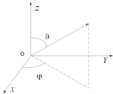
In order to simplify the derivation, a horizontal electric dipole is considered to revolve in theXOY plane. The length of electric dipole is denoted by l while its direction cosine α is as shown in Figure 1. The

position vector of the electric dipole in the uniﬁed coordinate system isr, andr =R0(ˆxcosβ+ ˆysinβ),

R0 is the distance between the phase center of the electric dipole and the origin of the coordinate system,

and β is the direction cosine of r. The deﬁnition of the coordinate system is shown in Figure 2.

Figure 1. Arbitrary oriented electric dipole in XOY plane.

Figure 2. The uniﬁed coordinate system.

The radiation amplitude vector of arbitrary current source is [10]

a

k

= k

4πj

V

_√ Z

¯

¯_I₋_ˆ_rˆ_r_·_J

r

ej

k·r

dv (1)

wherek=krˆ,k= 2π/λ,ˆris the radiation direction,Z the wave impedance, and λthe wavelength. The current distribution of electric dipole is expressed asJ(r) =Iˆland brought into Equation (1). Note that ˆl= ˆxcosα+ ˆysinα, then

a

˜ k

= kIl

√

Z 4πj

ˆ

θcosϑcos(α−ϕ) + ˆφsin(α−ϕ)

ejkR0sinϑcos(β−ϕ) (2)

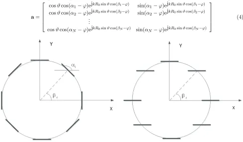
Considering thatN horizontal electric dipoles form a planar heterogeneous circular array in XOY plane, the radius isR0. The direction cosine angles of the electric dipoles areα1, α2, . . . , αN, and the direction

cosine angles of the position vector are β1, β2, . . . , βN, as shown in Figure 3. The radiation amplitude

(3)

Assuming that the mutual coupling of the antennas is not considered, the radiation amplitude vector of the ith element isa_i,

a_i(ϑ, ϕ) = kIl

√

Z 4πj

ˆ

θcosϑcos(αi−ϕ) + ˆφsin(αi−ϕ)

ejkR0sinϑcos(βi−ϕ)

, i= 1,2, . . . , N

Ignoring the factors unrelated to the direction,

a_i(ϑ, ϕ) = θˆcosϑcos(αi−ϕ) + ˆφsin(αi−ϕ)

ejkR0sinϑcos(βi−ϕ)

, i= 1,2, . . . , N (3) Formula (3) reﬂects the radiation amplitude, phase and polarization information inherent in the antenna, which is called the spatial response of the antenna. Its matrix form is given below,

a= ⎡ ⎢ ⎢ ⎢ ⎣

cosϑcos(α1−ϕ)ejkR0sinϑcos(β1−ϕ) sin(α1−ϕ)ejkR0sinϑcos(β1−ϕ)

cosϑcos(α2−ϕ)ejkR0sinϑcos(β2−ϕ) sin(α2−ϕ)ejkR0sinϑcos(β2−ϕ)

.. .

cosϑcos(αN−ϕ)ejkR0sinϑcos(βN−ϕ) sin(αN −ϕ)ejkR0sinϑcos(βN−ϕ)

⎤ ⎥ ⎥ ⎥

⎦ (4)

Figure 3. Heterogeneous array. Figure 4. Homogeneous arrays.

According to formula (3), the horizontal elements parallel to theXOY plane can receive not only the horizontal polarization components, but also the vertical polarization. Whenϑ=π/2, the array can only receive horizontal polarization for any azimuth. Whenα−ϕ=π/2, the array receives horizontal polarization for any pitch angle.

Considering that the incoming wave of signal is a fully polarized wave, the polarization state isuˆ.

ˆ

u = θˆcosγ0 + ˆφsinγ0ejη0, γ ∈ [0, π/2] and η ∈ [−π, π] represent the magnitude ratio and the phase

between the two polarization components [11]. γ = 0◦ represents the vertical polarization whileγ = 90◦ represents the horizontal polarization. According to the antenna receiving theory, the amplitude of the ith element receiving the unit ﬁeld strength is

Vi=ai·ˆu∗

where the sign (∗) represents conjugate. Then the manifold of the array is

A(ϑ, ϕ, γ, η) = ⎡ ⎢ ⎢ ⎣

cosϑcos(α1−ϕ) sin(α1−ϕ)

cosϑcos(α2−ϕ) sin(α2−ϕ)

.. .

cosϑcos(αN −ϕ) sin(αN −ϕ)

⎤ ⎥ ⎥ ⎦

N×2

cosγ0

sinγ0e-jη0

uH_{: 2}_×₁

⎡ ⎢ ⎢ ⎢ ⎣

ejkR0sinϑcos(β1−ϕ) ejkR0sinϑcos(β2−ϕ)

.. .

ejkR0sinϑcos(βN−ϕ) ⎤ ⎥ ⎥ ⎥ ⎦

N×1

(4)

where represents Schur-Hadamard.

Especially, if all direction cosine angles are the same,α1=α2 =. . .=αN =α0, then, the array is

a homogeneous array (see Figure 4), and the manifold becomes

A(ϑ, ϕ, γ, η) = ⎡ ⎢ ⎢ ⎢ ⎣

cosϑcos(α0−ϕ) cosγ0+ sin(α0−ϕ) sinγ0e-jη0

.. .

cosϑcos(α0−ϕ) cosγ0+ sin(α0−ϕ) sinγ0e-jη0 ⎤ ⎥ ⎥ ⎥ ⎦

N×1

⎡ ⎢ ⎢ ⎢ ⎣

.. .

N×1

Normalizing the magnitude, the manifold is

A(ϑ, ϕ, γ, η) = ⎡ ⎢ ⎢ ⎢ ⎣

.. .

N×1

(6)

where the manifold is not related to the polarization. Formula (6) is often used in the traditional DOA estimation based on circular array.

2.2. Spatial Correlation of the Manifold of Heterogeneous Array

Equation (2) can be rewritten further as follows

a_i =fi(ϑ, ϕ)ejζi(ϑ,ϕ)

ˆ

θcosγi+ ˆφsinγi

(7)

where fi(ϑ, ϕ) = [cosϑcos(αi−ϕ)]2+ [sin(αi−ϕ)]2 represents the amplitude pattern of the ith

element; ζi(ϑ, ϕ) = kR0sinϑcos(βi −ϕ) represents the phase pattern of the ith element; the phase

reference points is the coordinate origin.

cosγi= cosϑcos(αi−ϕ)

[cosϑcos(αi−ϕ)]2+ [sin(αi−ϕ)]2,

sinγi = sin(αi−ϕ)

[cosϑcos(αi−ϕ)]2+ [sin(αi−ϕ)]2,

LetU_i =θˆcosγi+ ˆφsinγi, which reﬂects the spatial polarization of the ith element. If the array

is a homogeneous array,U1=U2 =. . .UN.

Assuming that the directions of two incident waves areψ1 = (ϑ1, ϕ1) andψ2 = (ϑ2, ϕ2), respectively,

the corresponding polarization states areu1 andu2, respectively. Then the spatial correlation coeﬃcient

of these two incident waves for heterogeneous array is

ρ =

a(ψ1)uH1 _H

·a(ψ2)uH2

[a(ψ1)u1] · [a(ψ2)u2]

=

N

i=1

Fi(ψ1)Fi(ψ2)ej[ϕ(ψ1)−ϕ(ψ2)]

u1UH_i (ψ1)Ui(ψ2)uH2 N i=1

_F_i(ψ1)u1UH_i (ψ1) 2 · N i=1

_F_i(ψ2)u2UH_i (ψ2) 2

(8)

For the homogeneous array, the spatial correlation coeﬃcient is

ρ=

N

i=1

ej[ϕ(ψ1)−ϕ(ψ2)]

(5)

Obviously, for heterogeneous array, the correlation coefficient is related to wave polarized state. Two waves have different polarized states, and their spatial angles are close to each other. The correlation coefficient is less than 1 according to Schwartz inequality. However, for homogeneous array, its correlation coefficient is approximately equal to 1. The spatial correlation decreases in the heterogeneous array, which provides favorable conditions for distinguishing two signals in space. The smaller the spatial correlation coefficient is, the more favorable distinguishing signals will be [12].

3. DOA ESTIMATION BASED ON HETEROGENEOUS ARRAY

3.1. The Pol-MUSIC Methods Based on Heterogeneous Array

Assuming that there are D signals illuminating upon the heterogeneous array composed of N electric dipoles in the XOY plane (D < N). Then the time domain signal received by the elements can be written as follows

X =AS(t) +N(t) (10)

where N(t) is the Gaussian white noise. A = [a(ψ1)uH1 , a(ψ2)uH2 , . . . , a(ψD)uH_D] is the manifold of the

heterogeneous array (see formula (5)). S = [s1(t), s2(t), . . . , sD(t)]T. ψ1, ψ2, . . . , ψD are respectively the

directions ofDsignals, including the two dimension direction (ϑ, ϕ). u1, u2, . . . , uD are the polarizations

of the Dsignals.

Then the covariance matrix of the receiving data is

Rxx =ARsAH +σ2I (11)

Rs is the covariance matrix of the signals. When the signals are uncorrelated,Rs is a diagonal matrix. σ2 is the power of the noise.

According to the MUSIC subspace method [13], the span of the eigenvectors corresponding to theN -Dsmall eigenvalues ofR_XX is the noise subspaceE_KC, and the span of the eigenvectors corresponding to theD large eigenvalues ofR_XX is the signal subspace.

Using the orthogonal principle of signal subspace and noise subspace, the entire signal subspace including polarized space is projected into the noise subspace. In the true direction of the signal, the following equation holds:

uaHE_KC = 0 (12)

Further,

uaHE_KCEH_KCauH = 0 (13)

If DOA estimation is carried out directly using above equation, it is necessary to conduct a four-dimensional traversal search in the whole polarization domain and spatial domain. In fact, this process can be simpliﬁed. For a heterogeneous array,ais a full rank matrix with dimension ofN×2. Whatever the true polarization of the signal is, making Eq. (12) holds in the true direction of the signal, the matrixaHE_KCEH_KCawhose dimension is 2×2 must be rank deﬁcient. Namely,

detaHE_KCEH_KCa= 0 (14)

Operator symbol det{·} represents the determinant of matrix.

Therefore, the spatial spectral function based on heterogeneous can be constructed as below

P(ϑ, ϕ) = 1

detaH(ϑ, ϕ)E_KCEH_KCa(ϑ, ϕ) (15)

(6)

Once obtaining the DOA, the polarization information corresponding to the DOA can be obtained by searching in the polarization space according to formula (13). The polarization spectral function is displayed as follows

P(ψ0, γ, η) =

1

u(γ, η)aH(ψ0)EKCEH_KCa(ψ0)uH(γ, η)

(16)

where ψ0 is the DOA obtained from formula (15). In some scenarios, only the direction information is

required, and a two-dimensional search can be performed.

3.2. Numerical Simulation and Discussion

We consider that the array is a uniform circular array, which is composed of N electric dipoles in the XOY plane. βi = 2(i−1)π/N, i = 1,2, . . . , N. The radius of the circular array is R0. In the array,

electric dipole orientation is always tangent to the circumference while the direction cosine angle of the ith element isαi=π/2 +βi, i= 1,2, . . . , N. For a homogeneous array, α1 =α2 =. . . αN = 0, namely,

all electric dipoles are aligned and parallel to theX axis. To analyze the performance of heterogeneous array, we make a discussion in four aspects: correlation of the manifold, the accuracy of the proposed Pol-MUSIC, the resolution of two signals and the accuracy of DOA estimation for two signals.

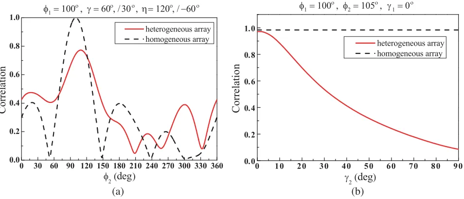
Example 1. Firstly, the spatial correlation of two incident signals is analyzed. Let the number of elements beN and the radiusR0 equal to 8 and 0.5λ, respectively. Assuming that azimuth of the ﬁrst

signal isϕ1 = 100◦, which is ﬁxed. The azimuth of the second signalϕ2 varies from 0◦ to 360◦ (pitching

angles of the two signals are 70◦,ϑ1 =ϑ2= 70◦). The polarizations of these two signals are orthogonal,

which are elliptically polarized waves, γ1 = 60◦, η1 = 120◦, γ2 = 30◦, η2 = −60◦. Figure 5(a) shows

the spatial correlation coeﬃcient variation with the azimuth of signal 2. In Figure 5(b), the spatial correlation coeﬃcient varies with the polarization of signal 2. Assume that the two signals are close to each other (ϕ1 = 100◦,ϕ2 = 105◦). In order to show the process of the polarization distance between

the two signals from minimum to maximum continuous change we choose theγ1 = 0◦,γ2 varying from

0◦ to 90◦, and η1 = η2 = 0◦. The polarization of signal 2 varies from vertical polarization wave to

horizontal polarization wave.

0 30 60 90 120 150 180 210 240 270 300 330 360 0.0

0.2 0.4 0.6 0.8 1.0

Correlation

φ₂( deg )

heterogeneous array homogeneous array

0 10 20 30 40 50 60 70 80 90

0.0 0.2 0.4 0.6 0.8 1.0

Correlatio

n

γ₂( deg)

heterogeneous array homogeneous array φ₁= 100 , ο _{γ = 60 , /}ο _{30 ,}ο _{η= 120 , /}ο ₋₆₀ο φ₁= 100 , ο φ₂= 105 , ο γ₁= 0 ο

(a) (b)

Figure 5. The spatial correlation based on the both array, (a) varying with azimuth ϕ, (b) varying with polarization γ.

(7)

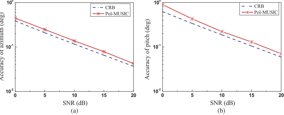
Example 2. Considering that there is only one signal in space, the estimation accuracy of the Pol-MUSIC method is veriﬁed by simulation. The number of elements N in the heterogeneous array is 8, and the radius of the circular array R0 is 0.5 lambda. The DOAs are ϑ = 70◦, ϕ = 100◦, and

its polarization parameters are γ = 60◦, η1 = 120◦. The four parameters are unknown and need to

be estimated. Sampling points of the signal are 1024 points, and the search angle interval is 0.2◦. We conduct 500 times Monte-Carlo simulations to estimate the azimuth and the pitch using formula (15). Figure 6 shows the variation curve of the estimation accuracy with the SNR. The simulation results show that the Pol-MUSIC method has a good accuracy based on the heterogeneous array, and the estimation results are close to the CRLB. The Pol-MUSIC is eﬀective.

0 5 10 15 20

10-2 10-1 100

Accuracy of azimuth (deg)

SNR (dB)

CRB Pol-MUSIC

0 5 10 15 20

10-2 10-1 100

Accuracy of pitch (deg)

SNR (dB)

CRB Pol-MUSIC

(a) (b)

Figure 6. Accuracy of DOA estimation using Pol-MUSIC. (a) Comparison of the azimuth accuracy of DOA estimation and CRB. (b) The pitch accuracy.

Example 3. The resolution probability of the heterogeneous array for two signals with a small angular separation is simulated. We deﬁne the resolution probability as the ratio of the number of times of the two signals which can be distinguished to the total number of experiments (ρ = Ndistinguished/Ntotal). Assume that the two signals are not relevant. The parameters of the array are

the same in example 2. Here, we compare three arrays: heterogeneous array, homogeneous array, and polarization-sensitive array of orthogonal dipole. The orthogonal dipole pair consists of an X-electric dipole and aY-electric dipole, which are respectively parallel to the X-axis andY-axis. 8 pairs of such orthogonal dipole antennas are distributed on the circumference of radius of 0.5λ. The polarization of signal 1 is γ1 = 60◦/η1 = 120◦, and the polarization of signal 2 is γ2 = 30◦/η2 = −60◦. The pitch

of the two signals are ϑ1 = ϑ2 = 70◦. Two azimuths are respectively ϕ1 = 100◦ and ϕ2 = 105◦.

Sampling points of the signals are 1024 points, and the search angle interval is 0.2◦. The total number of experiments is 500 times Monte-Carlo simulations.

In Figure 7(a), the MUSIC spectrum of the heterogeneous array is compared with the homogeneous array. The homogeneous array mistakenly identiﬁes two signals as one while the heterogeneous array accurately detects the two signals.

Figure 7(b) shows that the distinguish probability of two signals varies with the signal-to-noise ratio (SNR). In Figure 7(c), the function of distinguish probability is changed with the separation angle of the two signals. The direction of signal 1 is ﬁxed atϕ1= 100◦, and that of signal 2 varies from 101◦

(8)

0 30 60 90 120 150 180 210 240 270 300 330 360 -60

-50 -40 -30 -20 -10 0

80 90 100 110 120 130 140 -60

-50 -40 -30 -20 -10 0

MUSIC spe

ct

ru

m (d

B

)

Φ (deg)

heterogeneous array homogeneous array

DOA=100o/105o, SNR=10dB

0 5 10 15 20 25

-0.2 0.0 0.2 0.4 0.6 0.8 1.0

DOA=100o/105o

Probability of distinguish

SNR (dB)

heterogeneous array orthogonal dipole array homogeneous array

1 2 3 4 5 6 7 8 9 10

0.0 0.2 0.4 0.6 0.8 1.0

γ=60o/300,η=120o/-60o, SNR=10dB

DOA separation(deg)

0 10 20 30 40 50 60 70 80 90

0.0 0.2 0.4 0.6 0.8 1.0

polarization separation (deg) heterogeneous array orthogonal dipole array homogeneous array DOA=100o/105o, SNR=10dB

(a) (b)

(c) (d)

Figure 7. The ability of distinguish of two nearly signals. (a) The Pol-MUSIC spectrum, (b) the probability of distinguish two signals various by SNR, (c) the probability of distinguish two signals various by DOA separation, and (d) by the polarization separation of the two signals.

angle is 5 degrees. The results show that when two signal polarizations are orthogonal, the resolution probability of heterogeneous array is the highest.

Example 4. We analyze and compare the accuracy of two signals at the same time based on the heterogeneous array, homogeneous array and orthogonal dipole array. The accuracy is a function of the separation angle.

To make a fair comparison, we need to ensure that each array is able to distinguish the two signals with 100% probability. The separation angle varies from 12◦ to 60◦. Signal 1 is ﬁxed at ϕ1 = 100◦.

The pitch of the two signals are known and are the same, ϑ1 = ϑ2 = 70◦. The polarization states

of the signals are γ1 = 60◦/η1 = 120◦, γ2 = 30◦/η2 = −60◦. Figure 8 shows the variation curves of

DOA estimation accuracy with separation of azimuth angle. 500 times Monte-Carlo simulations are conducted in DOA estimation.

(9)

15 20 25 30 35 40 45 50 55 60 10-2

10-1

100 DOA1=100

o

, SNR=10dB

RMSE (deg)

DOA separation (deg)

15 20 25 30 35 40 45 50 55 60

10-2 10-1

100 DOA1=100

o

, SNR=20dB

RMSE (deg

)

DOA separation (deg)

(a) (b)

Figure 8. The accuracy of DOA estimation varying with DOA separation. The two polarizations of the signals are orthogonal. (a) SN R= 10 dB, (b)SN R= 20 dB.

has a lower spatial correlation. Moreover, the elements in homogeneous array are the same, all of which can eﬀectively participate in the array processing. In the three arrays, the estimation accuracy of the orthogonal dipole antenna array is the best. In orthogonal dipole antenna array, the number of channels is 2 times as that of the heterogeneous array, and its redundancy of data is larger. Therefore, it is theoretically more accurate than the heterogeneous array.

4. CONCLUSION

In this paper, a general expression of manifold of heterogeneous array is derived, and a new method of DOA estimation for signals with unknown polarizations is proposed. The proposed method does not need to search in polarization space to obtain accurate direction estimation, and the validity of this method is veriﬁed by simulation. The DOA estimation performance based on heterogeneous antenna array is discussed. For two signals with small angular separation, the heterogeneous array is easier to distinguish and has higher accuracy than the traditional homogeneous array. In addition, the heterogeneous array only needs one channel at each point of the spatial sampling to realize polarization sensitivity. The system complexity is reduced.

REFERENCES

1. Kornaros, E., S. Kabiri, and F. De Flaviis, “A novel model for direction ﬁnding and phase center with practical considerations,”IEEE Trans. Antennas Propag., Vol. 60, No. 10, 5475–5491, Oct. 2017.

2. Wang, M., X. Ma, and S. Yan, “An autocalibration algorithm for uniform circular array with unknown mutual coupling,”IEEE Antennas Wireless Propag. Lett., Vol. 15, 12–15, 2016.

3. Searle, S., “Disambiguation of interferometric DOA estimates in vehicular passive radar,” IET Radar, Sonar &Navigation, Vol. 12, No. 1, 64–73, Jan. 2018.

4. Yang, M., J. Ding, B. Chen, and X. Yuan, “A multiscale sparse array of spatially spread electromagnetic-vector-sensors for direction ﬁnding and polarization estimation,” IEEE Access, Vol. 6, 9807–9818, Jan. 2018

(10)

6. Wong, K. T., Y. Song, C. J. Fulton, S. Khan, and W.-Y. Tam, “Electrically “long” dipoles in a collocated/orthogonal triad — For direction ﬁnding and polarization estimation,” IEEE Trans. Antennas Propag., Vol. 65, No. 11, 6057–6067, Nov. 2017.

7. Meloling, J. H., J. W. Wockway, and M. P. Daly, “A vector-sensing antenna system, a high-frequency, vector-sensing array based on the two-port loop antenna element,” IEEE Antenna &

Propagation Magazine, 57–63, Dec. 2016.

8. Erthel, Y., “HF radio direction ﬁnding operating on a heterogeneous array: Principle and experimental validation,”Radio Science, Vol. 39, No. 1, 1–16, 2004.

9. Muller, R., S. Lutz, and R. Lorch, “A noel circular direction ﬁnding antenna array for unknown polariztion,” Proc. 7th Eur. Conf. Antennas Propag. (EuCAP), 1514–1518, Gothenburg, Sweden, Apr. 2013,

10. Loy, T. and S. W. Lee,Antenna Handbook, New York, Chapman&Hall, 1993.

11. Weiss, A. J. and B. Friedlander, “Analysis of a signal estimation algorithm for diversely polarized arrays,” IEEE Transactions on Signal Processing, Vol. 41, No. 8, 2628–2638, Aug. 1993.

12. Friedlander, B., “Antenna array manifolds for high-resolution direction ﬁnding,” IEEE Transactions on Signal Processing, Vol. 66, No. 4, 923–932, Nov. 2017.