A mesh free algorithm for ROF model

R E S E A R C H

Open Access

A mesh-free algorithm for ROF model

Mushtaq Ahmad Khan

, Wen Chen

, Asmat Ullah and Zhuojia Fu

Abstract

The total variation (TV) denoising method is a PDE-based technique that preserves the edges well but has undesirable staircase effect in some cases, namely, the translation of smooth regions (ramps) into piecewise constant regions (stairs). This paper introduces a novel mesh-free approach using TV (ROF model) regularization and radial basis function (RBF) for the numerical approximation of TV-based model to remove the additive noise from the measurements. This approach is structured on local collocation and multiquadric radial basis function. These features enable this strategy not only to eliminate noise from images and preserve the edges but also has the advantage to minimize the staircase effect substantially from real and artificial images which cause the image to look blocky. Experimental results

demonstrate that the proposed mesh-free approach is robust and performs well in visual improvement as well as peak signal-to-noise ratio compared with the recent partial differential equation (PDE)-based traditional methods.

Keywords: Image denoising, Total variation (TV) filter, Radial basis functions (RBF), Restoration equation, Mesh-based methods, Mesh-free method

1 Introduction

Image denoising is an inverse problem and is a very active area in the fields of image and signal processing that has been studied for the last three decades. Although there exist different types of noise, here we consider only mod-els for removing additive, zero-mean Gaussian noise. This can be modeled as

z=u+η, (1)

wherezis the given noisy image containing the unknown

additive noise (Gaussian noise) η and u is the known

actual image, all of which are defined on a domain ∈

R2. In literature, there are many effective numerical tech-niques have been utilized to tackle such models connected with image denoising having additive noise, for instance, in [1, 4, 13, 37, 44, 45].

The TV filtering [38] has proved to be one of the most successful tool in image processing for the solution of vari-ational based partial differential equation (PDE) restora-tion problems. In this method, it is supposed that the images are defined on a continuous domain, which results in continuous functional. This functional then leads to a Euler-Lagrange equation. The resulting PDEs are then

*Correspondence: [email protected]; [email protected] State Key Laboratory of Hydrology-Water Resources and Hydraulic Engineering, College of Mechanics and Materials, Hohai University, Nanjing, Jiangsu 210098, People’s Republic of China

discretized by existing classical numerical methods on a regular grid for smooth solutions. For more details about the TV filtering, see [22, 38, 39]. The first TV-based model for image restoration having additive noise was proposed by Rudin et al. (ROF) [38]. This model yields very satisfactory results for removing image noise while preserving edges, see [7, 37]. However, it also processes some unfavorable properties like staircase effect, loss of image contrast and in time computation due to its non-linearity and non-differentiability [5, 32, 33, 38]. In [38], the authors proposed an artificial time marching method to the associated Euler-Lagrange equation. This strategy is slow due to its strict stability constraints in the time steps. Also, the artificial time marching method computes the approximate solution, not the exact solution. Recently different procedures have been used to overcome this dif-ficulty and hence some good results have been obtained, for instance, see [14, 18, 29–31, 43, 46]. But still, there is space for improvement. So, in this work, we adapt the mesh-free BRF collocation method to reduce these issues. During the past decade, RBFs have been observed to be active techniques for the interpolation and approxi-mation of multi-variable smooth functions on scattered data sets [3, 6, 12]. More recently, an increasing attention has been given to the development of mesh-free methods using RBFs for the numerical solution of PDEs. Most PDEs results have concerned steady state problems with smooth

solutions. Recently there has been a growing interest in applying RBF methods to time-dependent PDE problems, again to problems with sufficiently smooth solutions. The RBF techniques have more points of interest and have exhibited superior accuracy as compared with tradi-tional numerical strategies, for example, finite difference method (FDM) [20, 23, 47], finite element method (FEM) [23], finite volume method (FVM) [21, 25], and pseudo-spectral method [24]. Interested readers can refer to [2, 8, 9, 16, 17, 26–28, 40] for more details about the RBF collocation methods.

Global RBF collocation technique is also easy to imple-ment, gives good accuracy and converges exponentially for solving the PDEs. Although, in this strategy, the inter-polation matrix is fully populated and ill-conditioned, and thus sensitive to shape parameter. Thus, it is com-putationally extremely expensive to apply global collo-cation method to large scale problems. So in literature, there are many domain type collocation techniques, for example, Kansa technique [19, 20] etc, is to settle these issues.

The main advantages of the RBFs for interpolating mul-tidimensional scattered data are discussed in [19, 20]. In recent decades, meshless methods have been proved to treat scientific and engineering problems efficiently. The mesh-free method based on the collocation method has been dominated and very efficient. Over the last several decades RBFs have been found to be widely successful for the interpolation of scattered data. RBF methods are not tied to a grid and in turn, belong to a category of meth-ods called mesh-free methmeth-ods. They apply only a cloud of points without any information about nodal connections. It is (conditionally) positive definite [3, 36, 42], rotation-ally and translationrotation-ally invariant. The RBF approximation is an incredibly powerful tool for representing smooth functions in non-trivial geometries since the method is mesh-free and can be spectrally accurate [10]. RBFs inter-polations have been used to remove the Gibbs oscillations from the given arbitrary data points [41] and very useful results have been obtained.

Motivated by the applications of TV-regularization in image restoration and RBF collocation methods for the solution of PDEs, we propose a new mesh-free strategy, with some modifications, of the TV (ROF) filter by RBF approximation to accomplish a new algorithm to solve the associated PDE with minimization of ROF model. This strategy is entirely mesh-less and is not only helpful to restore the image efficiently and resolve the edges due to is discontinuous jumps but also to eliminate the staircase effect and preserve the textures during the restoration process. The numerical treatment in this approach is also easy to implement and faster because of its mesh-free properties as compared to the traditional mesh-based numerical methods.

The rest of the paper is organized as follows. In Section 2, some details are provided related to the appli-cations of TV-regularization and its detail use in ROF model for image restoration. This section also contains the shortcoming in ROF model. This section also includes the details of RBFs and its applications in solving PDEs and comparison with traditional methods. Two mesh-based methods, i.e., implicit and Augmented Lagrangian meth-ods utilized for the solution of ROF model are presented in Section 3. This section also contains proposed method, i.e., BRF collocation method (Kansa method) for the solu-tion of the associated PDE with ROF model. Secsolu-tion 4, describes experimental results and discussion, to compare the three methods for ROF model regarding CPU times, the number of iterations, and quality (peak signal to noise ratio (PSNR)) of the restored images. This section also includes the shape parameter analysis on image restora-tion and comparison of the proposed method with an other recent method. Section 5, shows the tabulated dis-cussions about the sensitivity of parameters of the pro-posed method. The conclusion is provided in Section 6. And finally, the details for derivatives for our proposed method are given in an Appendix.

2 Related work

2.1 Total variation-based in image denoising Rudin-Osher-Fatemi (ROF) model

The TV regularization is a process in digital image pro-cessing for the noise removal and also an important tool in the inverse problem and numerical [15]. It is the only regularizer which is used to preserve the edges and for removing the highly noisy frequency components from the image. It is also a convex one. So the total variation (TV) for an imageu:→R2_{is defined as}

Rudin et. al (ROF) proposed the first model for image restoration from given noisy image having additive noise using TV regularization in [38]. This model achieved some useful restoration results.

The minimization approach for the model (1) using TV method is given as

u=argmin

corresponding Euler Lagrange equation of the ROF model (2) is given as follows;

− ∇.

marching restoration PDE from (3) is given as follows,

ut= ∇. ROF model has the following disadvantages.

• This model yields staircase effect, in restoring the smooth images in applications where edges are not the main features.

• This model also generates to the loss of image contrast during the restoration process. • This model also contains the difficulty with the

non-differentiability term in the total variation norm.

2.2 Radial basis functions approximation

RBFs are mostly multivariate functions, and their val-ues depend only on the distance from the origin, so that

φ(x) = φ(r) ∈ R, x ∈ Rn_{, r ∈ R; or alternatively on} the distance from a point of a given set {xj} such that

φ(x−xj)=φ(rj)∈R. Any functionφsatisfying the prop-ertyφ(x) = φ(x2)is called the radial function. Some commonly used, globally-supported RBFs are shown in Table 1.

RBF interpolation of a continuous multivariate function,

f(x),x ∈ ⊆ Rn, whereis the bounded domain. For

N interpolation function values {yi}N_i=1 ∈ Rat the data location (which are traditionally called centers in the RBF concept){xi}N_i=1∈⊆Rn, thenf(x)can be approximated by a linear combination of RBFs, namely,

f(x)= N

j=1

γjφ(x−xj2), x∈, (5)

whereγjare unknown coefficients which must be deter-mined. Using the collocation method, one may write:

yi=f(xi)= N

j=0

γjφ(xi−xj2), i,j=1, 2,. . .N.

The above linear system of equations can be expressed in the followingN×Nlinear system matrix form

Aα=b,

in whichα = (α1,α2,. . . αN)tis an unknown coefficient vector that should be determined,b=(y1,y2,. . .yN)t, and the RBF interpolation matrix is given by

A=[ij]=[φ(xi−xj2)]1≤i,j≤N with ij=ji,

where where A is a N ×N matrix, α and b areN ×1

matrices. However, some RBFs are conditionally positive definite functions as listed in Table 1, such as MQ, IMQ, GA, and TPS.

Hence, polynomials are augmented to Eq. (5) to guar-antee that the resultant interpolation matrix is invertible. Such a formulation is expressed as follows

f(x)=

Table 1[k] denotes the nearest integers less than or equal tok, andNthe natural number,ca positive constant which is known as the shape parameter, and CPD denotes the m-order conditionally positive definite functions [3, 11]

Name of RBF Definition CPD order (m)

Multiquadric (MQ) φ(r,c)=(r2_+c2₎k _{if k>0, k∈/N [k]+1}

Inverse multiquadric (IMQ) φ(r,c)=(r2_+c2₎−k _{if k>0, k∈/N 0}

Gaussian (GA) φ(r,c)=e−r

2

c2 ₀

Polyharmonic spline _φ(r₎₌

in whichpi ∈m−1, i = 1, 2,. . .,M, wherem repre-sents the polynomial space in which the total degree of all polynomials is thenminNvariables [36],

Moreover, details of positive definite (PD) and condi-tionality positive definite (CPD) RBFs are discussed in [3, 36] and listed in Table 1. For RBFs containing the shape parameterc, such as as in Table 1, small shape parameters produces more accurate results, but also associated with poorly conditioned interpolation matrix [3, 36].

3 Numerical methods for solution of ROF model

3.1 Implicit method (M1)

Rudin et al. (ROF) proposed the implicit scheme to solve the Eq. (4) in [38].

The numerical approximation for (4) is given as

uk_ij+1=ukij+ ther details, see [38].

3.2 Augmented Lagrangian method (M2)

Chunlin Wu [43] first proposed this numerical method in 2009, for the solution of ROF model (2) and hence many

good results have been obtained. So for this, he introduced a new variablepfor∇uand then separate the calculation of the non-differentiability term and the fidelity term. So the minimization problem (2) can be written as

u=argmin

which is constrained optimization problem.

So, the above problem (8) can be solved by Augmented Lagrangian method as andr is the positive constant. The system of optimality condition is written as follows

∂Lrof

The augmented Lagrangian process is used to solve (9), which is stated in the given Algorithm 1. To solve the

Algorithm 1 :Algorithm for Augmented Lagrangian method for the ROF model

1.ProcedureInput (u0=0,p0=0,χ0=0;)

For fixedpvalue,

and for fixeduvalue,

argmin

For the u-subproblem, the optimality condition is given by the following linear equation

λ(u−z)+divχk+rdivq−r∇u=0, (16)

which allows us to use the Fast Fourier transformF(u)and hence we get

The p-subproblem can be formulated as

argmin

and hence obtained the following closed solution

q= 1 solution of sub-problem (13). For further details, we refer

Algorithm 2 :Algorithm for Augmented Lagrangian method for the ROF model-solution of sub-problem (13). 1.ProcedureInput (uk+1,0=uk,pk+1,0=pk;)

3.3 Proposed method (M3)

In this subsection, our aim is to introduce a new algo-rithm, using both RBF interpolation and total variation norm to solve ROF model (4) and to reduce the difficulty associated with the total variation norm in ROF method (4). This methodology obviously uses advantages of both BRF interpolation and total variation norm which leads to the good restoration performance regarding restora-tion, eliminating the staircase effect, sharp edges and textures. Hence using this method, consistent improve-ment in PSNR values is obtained. Suppose{xi}N_i=1 is the

Ndistant evaluation points in ⊆ R2_{. So, for any radial} basis function the following equations satisfied,φ(r) = r2inR2, i.er = (x,y). For{xcj}Nc_j=1, givenNc centers, defining of radial basis function without polynomial term one may write:

ρj coefficients in RBF is determined via enforcing the interpolation condition

s(xj)=z,

a set of points that usually coincides withNccenters. The interpolation condition atNccenters results in aNc×Nc

linear system

Aρ=z

which must be solved for expansion coefficients of ρ. Whereρ = (ρ1,ρ2. . . ρNc)tandz = (z1,z2. . .zNc)t are

Nc × 1 matrices. The matrix A is called interpolation

matrix or system matrix, and is given by

A=[ij]=[φ(xi−xcj2)]1≤i,j≤Nc

This system matrixAisNc×Nc square and is always invertible [36] because it is always positive definite matrix [3, 34]. Hence we have

ρ=A−1z, (21)

whereρisNc×1 matrix. The interplant is evaluated using (20) at N evaluation points {xi}N

The interplant is then evaluated at N points using

matrix vector product to produceuas follows.

u=Bρ. (22)

Now, from Eqs. (21) and (22) the following equation is obtained.

u=BA−1z

or

u=Hz where H=BA−1, (23)

which gives approximate solution at any point in .

As in ROF model, the time marching Eq. (4) can be re-written as

u(n+1)−u(n)

dt =

u(xxn)

(u2

x)(n)+(u2y)(n)

+ u

(n) yy

(u2

x)(n)+(u2y)(n)

+λu(n)−z(0),t>0, (x,y)∈R, or

u(n+1)−u(n)

dt =

1

(u2

x)(n)+(u2y)(n)

u(_xxn)+u(_yyn)

+λ(u2

x)(n)+(u2y)(n)

u(n)−z(0)!,

t>0, (x,y)∈R,

(24)

Now, combining Eqs. (24) and (23) we get a new restora-tion PDE, which is shown in the undergoing non-linear system of equations:

Lu(n)u(n+1)=Lu(n)u(n)+dt u(_xxn)+u_yy(n)+Lu(n)

λu(n)−z(0)!,t>0, (x,y)∈R, (25)

whereL(u)=u2

x+u2y,ux=Hxz,uxx=Hxxz,uy=Hyz, uyy=Hyyz, ∂_∂u_n =un=Hnz, andz(0)=z.

Since the RBF in the Kansa scheme does not necessarily satisfy the governing Eq. (25), so we have more freedom to choose a RBF. The most popular RBF in the Kansa method is the multiquadric (MQ) [20, 34], which usually shows spectral accuracy if an appropriate shape parametercis chosen. Here, the shape parametercused in RBF is also one of the most important parameters for the smooth-ness in our method M3. For the optimal value ofc, our proposed methodology gives more accurate and smooth results in image denoising having additive noise. In this technique the shape parametercand fitting parameterλ depend on the size of the image and the noise level in the image.

Algorithm 3:Algorithm for proposed method M3

RBF

1. SetN=Nc,ntotal number of pixel points (N shows the image size i.e.,N×N), whereNandNcare called the total number of pixel and center pixel points which are used in the RBF approximation process.

2. Find theρaccording to (21) by multiquadric radial basis function (MQ-RBF) by using step (1).

3. Finduaccording to (23) by MQ-RBF by using steps (1) and (2).

TV filtering

4. Initialize the values ofλ,,c,dt, andz.

5. SetnasNccenters pixel points i.e.xc1≤xc2≤. . .xcn, setn=0.

6. Atn = 0, putuas MQ-RBF matrix in (25) from (23). Where we choosez(0)=z.

7.n=n+1. For each center pointxci, fori=1, 2, 3. . .n, computeu(n+1)according to (25) by Kansa method. 8. u(n_u+1)(n−u)(n) ≤ = 10−5(stopping criteria), go to step

(10).

9. Go to step (7). 10. End.

11. Outputu=u(n+1).

4 Results and discussion

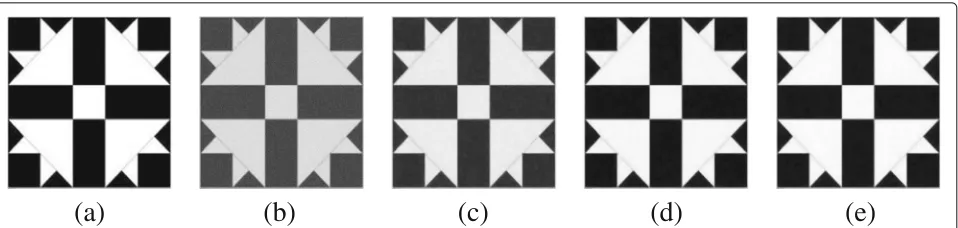
In this section, some numerical results are provided to demonstrate the performance of our proposed method M3. Obtained results are compared with the results of methods M1 and M2. The test images are “Lena”, “Par-rot”, “Synthetic1”, “Synthetic2”, and “Cameraman” which are shown in Fig. 1.

In this paper, it is assumed thatN = Nc =the size of the image, for our method M3, for the sake of compari-son with methods M1 and M2. Here, Multiquadric radial basis function (MQ-RBF) is utilized for the proposed method M3. To quantify the denoised image, the peak-signal-to-noise ratio (PSNR) is considered. This measure has been commonly used and applied to determine the

(a)

(b)

(c)

(d)

(e)

quality of the restored image. The following formula can calculate it.

PSNR=10∗log₁₀

M×Nmax{ˆu}2 ˆu−u2

(26)

Whereuˆis the given image,uis the restored image and

M×Nis the size of the image. Iterations in our algorithm are terminated when the following condition is satisfied.

u(k+1)−u(k)

u(k) ≤, (27)

whereindicates the maximum permissible error. Here, it is set to be 10−5.

Here we use the Multiquadric (MQ) RBF to test and compare the results of method M3 with methods M1 and M2. For each point (xj,yj), Multiquadric (MQ) RBF is defined as equation below.

φj(x,y)=

c2_+r2

j =

c2_+(x−xj)2_+(y−yj)2_,

whererj=

(x−xj)2+(y−yj)2.

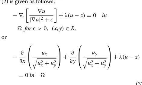
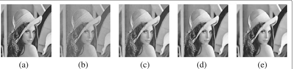
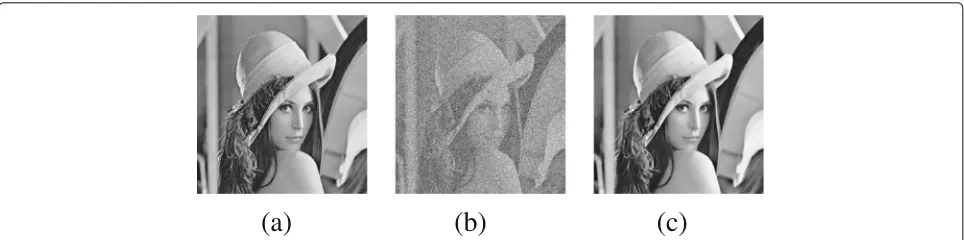
Example 1: In this first example, the three methods, M1, M2, and M3 are applied and tested on natural images “Lena” and “Parrot” with additive noises (Gaussian noise with mean value zero and standard deviationσ) with noise levelsσ =20, andσ =18, which are shown in the Figs. 2 and 3, respectively. In all three figures, (a) and (b) are the original and noisy images while (c), (d), and (e) depict the restored images by the three methods M1, M2, and M3, respectively. In each case, we can clearly notice that the visual quality of restoration by proposed method M3 is quite efficient than that of methods M1 and M2. Method M1 can restore the images, but the quality of restored images are not so good. Also, it creates staircase effect, which is an intrinsic defect of the TV regularization in ROF method as discussed in [7, 35]. These reconstructed images are shown in the Figs. 2c and 3c, respectively. In M2, the visual quality of the restored images are good as compared with the method M1. But still, it contains

the staircase effect due to the TV regularization. These obtained images are shown in the Figs. 2d and 3d, respec-tively. In our method M3, the visual quality, preservation of edges, and the minimization of staircase effect of the restored images are far better than that of methods M1 and M2 due to the mesh-free characteristics of MQ-RBF approximation used in our method M3. These denoised images are shown in the Figs. 2e and 3e, respectively. In our method M3, the shape parametercplays a vital role in image denoising. The range of optimal value forc in

this example is set to 1.63 ≤ c ≤ 1.70. Moreover, the

PSNR values for the two images “Lena” and “Parrot” for three methods M1, M2, and M3 are listed in Table 2. The bigger the PSNR value, the better the denoising perfor-mance. It can be seen from Table 2 that the PSNR values of method M3 are greater than that of methods M1 and M2 for the two images, which shows the dynamic restoration performance of the M3 over M1 and M2. The CPU time of computation and number of iterations required for con-vergence of the three methods M1, M2, and M3 are also listed in Table 3. It can be observed from Table 3 that the number of iterations and CPU time of computation of the M3 is smaller than that of M1 and M2, which shows the faster restoration performance of our mesh-free algorithm of proposed model M3 over the mesh-based algorithms M1 and M2. The best experimental optimal values of parameters of our technique M3 (shape parameter (c) and fitting parameter (λ) ) for the two images “Lena” and “Par-rot” are (1.69, 15.5) and (1.65, 14.7), respectively. So, it is evident from this example, that the performance of our free based method M3 is superior to that of mesh-based methods M1 and M2 regarding visual restoration quality ( PSNR), the number of iterations, and CPU time of computation.

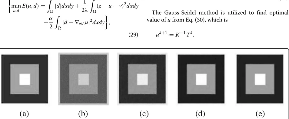
Example 2: In this second example, we study how our algorithm M3 deals with the synthetic images “SynIm-age1” and “SynImage2” having the Gaussian noises. These synthetic images are listed in the Figs. 4 and 5, respec-tively. The noise level for the two artificial images

“synIm-age1” and “synImage2” in this example areσ = 18 and

(a)

(b)

(c)

(d)

(e)

(a)

(b)

(c)

(d)

(e)

σ = 16, respectively. Again in both cases, the efficiency of the restoration of M3 (shown in Figs. 4e and 5e, tively) is better than M1 (shown in Figs. 4c and 5c, respec-tively) and M2 (shown in Figs. 4d and 5d, respecrespec-tively). In this example, the best experimental optimal values of the parameters used for the two images “SynImage1”, and “SynImage2” are for proposed technique M3 (shape parameter (c) and fitting parameter (λ)) are (1.76, 15.3) and (1.73, 13.9), respectively. Again, the range of the opti-mal value of shape parametercfor our proposed method M3 in this example is set to 1.72≤c≤1.77. The perfor-mance of the three methods M1, M2, and M3, concerning restoration (PSNR values), CPU computation time, and number of iterations required for convergence for the two images, i.e., “SynImage1” and “SynImage2”, are recorded in Tables 2 and 3, respectively. Again, from Tables 2 and 3, M3 shows adequate performance than M1 and M2 due to the mesh-free applications of MQ-RBF used in our algorithm M3.

Example 3: In this example, the three methodologies M1, M2, and M3 are applied and tested on “Cameraman” having different noise levels. Here, we can observe that the visual quality of restoration (PSNR) of our proposed approach M3 is much better than that of M1 and M2 because of mesh-less applications of MQ-RBFs employed in our proposed method M3 especially when the noise

Table 2Comparison of methods M1, M2, and proposed method M3 in terms of PSNR

Image Size Method M1 Method M2 Method M3

PSNR PSNR PSNR

Lena 4002 _{24.96 25.47 26.01}

Parrot 4002 _{26.89 27.55 28.04}

SynImag1 4002 _{28.31 29.11 29.87}

SynImag2 4002 26.15 27.33 27.95

variance is significant. These can be seen from Figs. 6, 7, 8, and Table 4, respectively.

Example 4: In this fourth example, we evaluate the performance of three algorithms, M1, M2, and M3, in regions that are dominated by discontinuities by the piecewise contact signals which are shown in Fig. 9. In areas with edges, we observe that M3 restores and enhances these image features in a productive way com-pared to M1 and M2, which shows the better per-formance of edge enhancement of M3 over M1 and M2. These results are shown in Fig. 9c, d, and e, respectively.

Example 5: In this example, we compare the three techniques, M1, M2, and M3, for texture persevera-tion that are given in Fig. 10. Here, we observed that the textured regions were sufficiently reconstructed by using the M3 as compared to M1 and M2 because of the effectiveness to our proposed method M3. These reconstructed results are shown in Fig. 10c, d, and e, respectively.

Example 6: Here, the homogeneity is checked, and loss (or preservation) is examined for the three techniques M1, M2, and M3 while being applied to “Lena”. For this pur-pose, different lines of the original image compared with noisy and restored images that are shown in Figs. 11 and 12. It is clear that the lines restored by proposed method M3 (shown in Figs. 11d and 12d) are far better than what acquired utilizing methods M1 and M2 that are presented in the figures (Figs. 11c and 12c) and (Figs. 11b and 12b), respectively. The blue line is the original image, and red line is the restored image.

4.1 Shape parameter analysis

In this subsection, we compare the image restoration (PSNR) by our proposed method M3 for the different values of shape parametercfor real and artificial images.

Table 3Comparison of methods M1, M2, and proposed method M3 in terms of number of iterations (Iters) and CPU-time (Time) in seconds

Image Size Method M1 Method M2 Method M3

Iters Time (s) Iters Time (s) Iters Time (s)

Lena 4002 _{32 27.11 21 16.30 15 11.82}

Parrot 4002 29 23.71 18 13.79 12 9.36

SynImag1 4002 35 31.50 24 20.57 19 14.47

SynImag2 4002 31 28.35 22 18.52 16 12.91

artificial images shown in Figs. 13 and 14. The PSNR val-ues of the two images are also listed in Table 5 for different values of shape parameters.

4.2 Comparison with an other recent model

Dong et.al proposed a new variational model for image restoration in 2015 [18], and some good restoration results have been obtained on real images. The minimization functional of this model is given as

min

u,v E(u,v)=

|∇NLu|dxdy+ α

2

|∇NLv| 2_dxdy

+ 1 2λ

(z−u−v) 2_dxdy,

(28)

wereαandλare the two regularization parameters. This

model can be written a decomposition model as z =

u+v+w. Here,u,v, andware taken as discontinuous, piecewise smooth, and noise components, respectively. By alternating minimization technique and unconstrained transformation technique the author gets the following minimization functional.

" min

u,d E(u,d)=

|d|dxdy+ 1 2λ

(z−u−v) 2_dxdy

+α 2

|d− ∇NLu| 2_dxdy

# ,

(29)

where d = ∇NLu. The split Bregman applied for the

solution of functional (29), which is given as

uk+1=argmin u

"

1

2λz−u−v 2 2+

α

2d k_{− ∇}

NLu−bk22

#

(30)

dk+1=argmin d

"

|d|dxdy+ α

2d

k_{− ∇NLu−b}k2 2 #

(31)

bk+1=bk+

∇NLuk+1−dk+1

(32)

The associated Euler Lagrange equation of subproblem (30) foruis

1

λI−α∇NL

uk+1= 1

λ(z−v)+αdivNL

dk−bk

.

(33)

The Gauss-Seidel method is utilized to find optimal value ofufrom Eq. (30), which is

uk+1=K−1Tk,

(a)

(b)

(c)

(d)

(e)

(a)

(b)

(c)

(d)

(e)

(a)

(b)

(c)

(d)

(e)

Fig. 6Denoised results on “Cameraman” image;atrue image;bnoisy image withσ=24;cprocessed with method M1;dprocessed with method M2;eprocessed with method M3

(a)

(b)

(c)

(d)

(e)

Fig. 7Restored results on “Cameraman” image;aoriginal image;bnoisy image withσ=22;crestored image by method M1;drestored image by method M2;erestored image by method M3

(a)

(b)

(c)

(d)

(e)

Table 4Comparison of PSNR value of the restored image “Cameraman” for different additive noise values for three algorithms M1, M2, and M3

Image σ =24 σ =22 σ =20

M1 M2 M3 M1 M2 M3 M1 M2 M3

Cameraman (PSNR) 19.83 20.90 21.29 20.57 21.42 21.94 21.76 22.47 23.01

where

K= 1

λI−α∇NL,

and

Tk = 1

λ(z−v)+αdivNL

dk−bk

.

The optimal value ofdcan be defined as

dk+1=shrink∇NLuk+1

,

whereshrink(x,γ )= |x|_x .max(|x| −γ, 0). For more infor-mation, see [18].

Here, we compare our proposed method M3 with a recent method [18] described above. We can notice that the display results in Figs. 15, 16, and 17 and Table 6 that our model M3 performs well regarding visual quality of restoration (PSNR) than method [18] for the same noise variance taken in method [18].

5 Sensitivity analysis of parameters

To comment briefly on the choice of the shape parame-ter (c) and fitting parameter (λ) used in the algorithm M3 described above, it is recommended from our experience that all the two parameterscandλare more complicated to choose. However, its optimal values are adjusted and tuned according to the noise variance, image size, etc. It has been observed that the range of values allowed are

c ∈[ 1.63, 1.78] andλ ∈[ 13.2, 16.3], for natural and arti-ficial images. It indicates that all the parameters c and

λ are more important for improving denoising

perfor-mance. Similarly, the number of iterations required for convergence are taken to be in the range [ 7, 27] for results with improved PSNR. Thus, the availability of information about the uncertainty of the denoising result on the user-chosen parameters (by Trial and Error Method) is helpful to avoid incorrect decisions.

For brevity, for Tables 7 and 8 we shall denote by

1. (·)%increase− ↑, and(·)%decrease− ↓

2. For example(0.17)↓stands for 0.17% decrease in PSNR

3. (0.21)↑stands for 0.21% increase in PSNR

6 Conclusions

In this paper, a new TV based mesh-free algorithm for additive noise removal is presented in which TV regularization (ROF model) is employed in conjunction with MQ-RBF approximation. This algorithm is exploited for the solution of non-linear PDE arisen from the mini-mization of the associated TV functional of ROF model. The proposed algorithm (Kansa method) is mathemati-cally simple and robust compared with the classical mesh-based methods and hence provide more optimal results because of mesh-free applications of MQ-RBF associated with his algorithm.

This approach is tested on different artificial and real images for additive noise, and the results are compared with the existing methods. Our experimental results have

(a)

(b)

(c)

(d)

(e)

(a)

(b)

(c)

(d)

(e)

Fig. 10Experimental results on synthetic texture image;aoriginal image;bnoisy image;crestored image by method M1;drestored image by method M2;erestored image by method M3

Fig. 11The 57th line comparison of original image with noisy image, restored image by model M1, restored image by method M2, and restored image by method M3 of the “Lena”.aOriginal and noisy image lines;boriginal and restored by method M1 image lines;coriginal and restored by method M2 image lines;doriginal and restored by method M3 image lines. Theblue lineis the original image, andred lineis the restored image

Fig. 12The 99th line comparison of original image with noisy image, restored image by model M1, restored image by method M2, and restored image by method M3 of the “Lena”.aOriginal and noisy image lines;boriginal and restored by method M1 image lines;coriginal and restored by method M2 image lines;doriginal and restored by method M3 image lines. Theblue lineis the original image, andred lineis the restored image

(a)

(b)

(c)

(d)

(e)

Fig. 13Denoised results on Lenaaoriginal image;bLena image corrupted with Gaussian noise withσ =20;crestored image by optimal value of

(a)

(b)

(c)

(d)

(e)

shown that the quality of the restoration of images, the number of iterations, and the CPU times with the use of the proposed method are quite good, and the proposed algorithm is quite efficient. We have also noticed that the performance of our proposed method is far better than that of the existing methods regarding restoration quality (PSNR), the number of iterations, and CPU times because of the mesh-free properties of RBF used in our algorithm. The choice of shape parametercalso plays a significant role in this algorithm, which affects the image restoration. The shape parameter analysis has also been discussed here. A comparison with another method in this field is provided as well.

However, this method produces an unsymmetri-cal interpolation matrix. Additionally, sometimes, this approach suffers relatively lower accuracy in boundary-adjacent regions. These problems are under intense study and results will be reported in the subsequent paper.

Appendix

The derivatives in our method M3 for Eq. (25) are given as under: Since Eq. (21) is

ρ=A−1z, (34)

When we evaluate the derivative atN evaluation points

{xi}N_i=1andNccenter points

{xj}Nc_j=1

, then RBF inter-polation, we have

u= Nc

j=1

ρjφ(x−xcj2), (35)

or

u=Bρ, (36)

with (N×Nc) evaluation matrixB, i.e.,

B=[ij]=[φ(xi−xcj2)] for i=1,2,...N, j=1,2,..Nc.

Then, the derivative becomes from (35) is as follows:

∂u ∂xi =

Nc

j=1 ρj ∂

∂xiφ(

x−xcj2), (37)

or

∂u ∂xi =

∂ ∂xi

Bρ. (38)

Where

∂B ∂xi=

∂[ij] ∂xi =

∂ ∂xi

[φ(xi−xcj2)] for i=1,2,...N, j=1,2,..Nc.

Combining Eqs. (34) and (38) we have

∂u ∂xi =

∂ ∂xi

BA−1z. (39)

Table 5Comparison of the image quantity (PSNR values) for different values (increase and decrease) in shape parametercwith the optimal value of shape parametercof the proposed method M3 for real and artificial images

Image Size Optimal valuec PSNR Increasec PSNR Decreasec PSNR

Lena 4002 _{1.69 26.01 1.78 25.57 1.61 25.29}

(a)

(b)

(c)

Fig. 15Denoised result on Lena;atrue image;bnoisy image with Gaussian noise with_σ=15 ;cprocessed with method M3

(a)

(b)

(c)

Fig. 16Reconstructed result on cameraman;atrue image;bnoisy image with Gaussian noise withσ=20 ;cdenoised with method M3

Table 6Comparison of our method M3 with the model [18] in terms of PRNR

Image Size Method [18] Method M3

PSNR PSNR

Lena 2562 _{30.9162 31.2413}

Cameraman 2562 28.6519 30.3126

Barbara 2562 26.5676 27.9471

DefineH = BA−1, then above equation (39) can be

re-The differentiation matrix can be defined as

Hxi=

∂ ∂xi

BA−1=BxiA−1. (41)

For second derivative, we have

Hxixi=

The differentiation matrix is well-defined since it is known that the system matrixAis invertible.

For any sufficiently differentiable RBF,φ[r(x)], the chain rule gives

for the first derivative, with

∂r ∂xi =

xi

r. (45)

The second derivative is calculated as follows

∂2_φ

Table 7PSNR value of the restored image “Lena” with optimal values ofcandλis 26.01. Parameter sensitivity analysis for our proposed method M3 by percentage increased in values of the parameterscandλ, with the resultant percentage increase or decrease in PSNR of the denoised image of size(4002₎

Image 30% (↑) 60% (↑)

c λ PSNR c λ PSNR

Lena 2.20 20.15 2.26(↓) 2.71 24.80 3.93(↓)

Table 8PSNR value of the restored image “Lena” with optimal values ofcandλis 26.01. Parameter sensitivity analysis for our proposed method M3 by percentage decreased in values of the parameterscandλ, with the resultant percentage increase or decrease in PSNR of the denoised image of size(4002₎

Image 30% (_↓) 60% (_↓)

c _λ PSNR c _λ PSNR

Lena 1.18 10.85 2.57_(↓) 0.68 6.20 4.81_(↓)

For the MQ in particular,

dφ

The work described in this paper is supported by the China Scholarship Council (CSC), the National Science Funds of China (Grant Nos. 11572111, 11372097) and the 111 Project (Grant No. B12032). This paper does not necessarily reflect the views of the funding agencies.

Authors’ contributions

All the three authors have contributed equally to the text, while MAK has implemented the algorithms and performed most of the tests. All the three authors read and approved the final manuscript.

Competing interests

The authors declare that they have no competing interests.

Publisher’s Note

Springer Nature remains neutral with regard to jurisdictional claims in published maps and institutional affiliations.

Received: 8 January 2017 Accepted: 27 June 2017

References

1. G Aubert, P Kornprobst, Mathematical problems in image processing. Appl. Math. Sci, 147 (2006). doi:10.1007/b97428

2. F Bernal, G Gutiérrez, Solving delay differential equations through RBF collocation. AAMM.1(2), 257–272 (2009). doi:arXiv:1701.00244 3. MD Buhmann, Radial basis functions: theory and implementations.

Cambridge Monogr. Appl. Comput. Math (2003). doi:10.1017/CBO9780511543241

4. A Chambolle, PL Lions, Image recovery via total variational minimization and related problems. Num. Math. Springer.76(2), 167–188 (1997). doi:10.1007/s00211005025

5. Q Chang, X Ta, L Xing, A compound algorithm of denoising using second-order and fourth-order partial differential equations. NM-TMA.

2(4), 353–376 (2009). doi:10.4208/nmtma.2009.m9001s 6. W Chen, ZJ Fu, CS Chen,Recent advances in radial basis function

collocation, (2013). doi:10.1007/978-3-642-39572-7

7. TF Chen, S Esedoglu, F Park, A Yip,Total variation image restoration. Overview and recent developments. (N Paragios, Y Chen, O Faugeras, eds.) (Springer, New Yark, 2006), pp. 17–31. doi:10.1007/0-387-28831-7 8. Y Chen, S Gottlieb, A Heryudono, A Narayan, A reduced radial basis

function method for partial differential equations on irregular domains. J. Sci. Comp. Arc.66(1), 67–90 (2016). doi:10.1007/s10915-015-0013-8 9. M Dehghan, M Abbaszadeh, A Mohebbi, A meshless technique based on

parabolic-parabolic-patlak-keller-segal-chemotaxis model. Eng. Anal. Bound. Elem.56, 129–144 (2015). doi:10.1016/j.enganabound.2015.02.005 10. TA Driscoll, B Fornberg, Interpolation in the limit of increasingly flat radial

basis functions. Comput. Math. App.3-5(43), 413–422 (2002). doi:10.1016/j.jcp.2015.12.015

11. N Dyn, Interpolation and approximation by radial and related function. Approx. Theo.1, 211–234 (1989). doi:10.1007/BF01203417

12. GE Fasshauer, Solving partial differential equations by collections with radial basis functions. Appl. Math. Comp.93, 73–82 (1998).

doi:10.1023/A:1018919824891

13. S Geman, D Geman, Stochastic relaxation, Gibbs distributions, and the bayesian restoration of images. IEEE Trans. Pattern Anal. Mach. Intell.6(6), 721–741 (1994). doi:10.1109/TPAMI.1984.4767596

14. T Goldstein, S Osher, The split bregman method for L1-regularized problems. SIAM J. Imaging Sci.2(2), 323–343 (2009).

doi:10.1137/080725891

15. Y Huang, MK Ng, YW Wen, A fast total variation minimization method for image restoration. Multiscale Model. Simul.7(2), 774–795 (2007). doi:10.1137/070703533

16. SU Islam, V Singh, S Rajput, Estimation of dispersion in an open channel from an elevated source using an upwind local meshless method. Inter. J. Comp. Meth (2016). In Press, doi:10.1142/S0219876217500098

17. SU Islam, B Sarler, R Vertnik, Local radial basis function collocation method along with explicit time stepping for hyperbolic partial differential equations. Appl. Num. Math.67, 136–151 (2013).

doi:10.1016/j.apnum.2011.08.009

18. DH Jiang, X Tan, YQ Liang, S Fang, A new nonlocal variational bi-regularized image restoration model via split bregman method. EURASIP. J Image. Vide. Process.15(1) (2015). doi:10.1186/s13640-015-0072-7 19. EJ Kansa, Multiquadrics-a scattered data approximation scheme with

applications to computational fluid dynamics I: solutions to parabolic, hyperbolic, and elliptic partial differential equations. Comput. Math. App.

19, 147–161 (1990). doi:10.1016/0898-1221(90)90270-T

20. EJ Kansa, Multiquadrics-a scattered data approximation scheme with applications to computational fluid dynamics II: surface approximations and partial derivative estimates. Comput. Math. App.19, 127–145 (1990). doi:10.1016/0898-1221(90)90271-K

21. (EJ Kansa, ed.),Motivation for using radial basis functions to solve PDEs. (LLNL, USA, 1999). doi:10.1007/s11075-012-9675-6

22. D Krishnan, P Lin, XC Tia, An efficient operator-splitting method for noise removal in images. Commun. Comput. Phys.1(5), 847–858 (2009) 23. E Larsson, B Fornberg, On the efficiency and exponential convergence of

multiquadric collocation method compared with finite element method. Eng. An. Bound. El, 251–257 (2003). doi:10.1016/S0955-7997(02)00081-4 24. E Larsson, B Fornberg, A numerical study of some radial basis function

based solution methods for elliptic PDEs. Comp. Math. Appl.46, 891–902 (2003). doi:10.1016/S0898-1221(03)90151-9

25. J Li, YC Hon, Domain decomposition for radial basis meshless methods. IEEE Trans. Commun.31, 388–397 (1983). doi:1002/num.10096 26. K Liu, M Xu, Z Yu (eds.),Feature-preserving image restoration from adaptive

triangular meshes, vol. 9009(ACCV. Springer, 2014), pp. 31–46. arXiv:1406.7062

27. K Liu, Xu M, Z Yu, Adaptive mesh representation and restoration of biomedical images. Eur. J. Anaesthesiol.31(1), 589–596 (2014). doi:https:// pantherfile.uwm.edu/yuz/www/bmv/index.html

28. (K Liu, ed.),Radial basis functions: Biomedical applications and parallelization. Theses and Dissertations. (Ke Liu University of Wisconsin-Milwaukee, 2016)

29. X Liu, L Huang, A new nonlocal total variation regularization algorithm for image denoising. Math. Comput. Simulat.97(1), 224–233 (2014). doi:10.1016/j.matcom.2013.10.001

30. X Liu, L Huang, An efficient algorithm for adaptive total variation based image decomposition and restoration. Int. J Appl. Comput. Sci.24(2), 405–415 (2014). doi:10.2478/amcs-2014-0031

31. X Liu, L Huang, Total bounded variation-based Poissonian images recovery by split bregman iteration. Math. Method. Appl. Sci.35(5), 520–529 (2012). doi:10.1002/mma.1588

32. M Lysaker, S Osher, XC Tai, Noise removal using smoothed normals and surface fitting. IEEE trans. Image Process.13(10), 1345–1375 (2004). doi:10.1109/TIP.2004.834662

33. M Lysaker, A Lundervold, XC Tai, Noise removal using fourth-order partial differential equation with application to medical magnetic resonance images in space and time. IEEE Trans. Image Process.12(12), 1579–1590 (2003). doi:10.1109/TIP.2003.819229

34. WR Madych, SA Nelson,Multivariate interpolation: a variational theiry. (MIT Press, Cambridge, Mass, 1983). doi:10.1007/BFb0072406

35. Y Meyer,Oscillating patterns in image processing and nonlinear evolution equations: the fifteenth Dean Jacqueline B. Lewis memorial lectures. (Uni. Lecture Series, AMS, 22, 2001). doi:http://dx.doi.org/10.1090/ulect/022 36. CA Micchelli, Interpolation of scattered data: distance matrices and

conditionally positive definite functions. Constr. Approx.2, 11–12 (1986). doi:10.1007/BE01893414

37. S Osher, M Burger, D Goldfarb, J Xu, W Yin, An iterative regularization method for total variation-based image restoration. Multiscale Model Simul.4(2), 460–489 (2005)

38. LI Rudin, S Osher, E Fatemi, Nonlinear total variation based noise removal algorithms. Physica D.60, 259–268 (1992).

doi:10.1016/0167-2789(92)90242-F

39. L Rudin, S Osher, Total variation based image restoration with free local constraints. IEEE Trans. Image Process.1, 31–35 (1994).

doi:10.1109/ICIP.1994.413269

40. S Sajavicius, Optimization, conditioning and accuracy of radial basis function method for partial differential equations with nonlocal boundary conditions. Eng. Anal. Bound. Elem.37(4), 788–804 (2013).

doi:10.1016/j.enganabound.2013.01.009

41. SA Sarra, Digital total variation filtering as postprocessing for radial basis function approximation methods. Comput. Math. App.52, 1119–11130 (2006). doi:10.1016/j.camwa.2006.02.013

42. SA Sarra, Multiquadric Radial Basis Function Approximation methods for the numerical solution of partial differential equations. Adv. Appl. Mech (2009). doi:10.1016/S0021-9991(03)00089-5

43. XC Tai, C Wu, Augmented lagrangian method, dual methods, and split bregman iteration for ROF model. SSVM Springer.5567, 502–513 (2009). doi:10.1007/978-3-642-02256-2-42

44. LA Vase, SJ Osher, Modeling texture with total variation minimization and oscillating pattern in image processing. J. Sci. Comput.19, 1–3 (2003). doi:10.1023/A:1025384832106

45. Y Wang, J Yang, W Yin, Y Zhang, A new alternating minimization algorithm for total variation image reconstruction. SIAM J. Imaging. Sciences.1(3), 248–272 (2008). doi:10.1137/080724265

46. H Xu, Q Sun, N Luo, G Cao, D Xia, Iterative nonlocal total variation regularization method for image restoration. PLOS ONE.8(6), e65865 (2013). doi:10.1371/journal.pone.0065865